Viscous Hydrodynamic Description of the Pseudorapidity Density and Energy Density Estimation for Pb+Pb and Xe+Xe Collisions at the LHC


Abstract
:1. Introduction
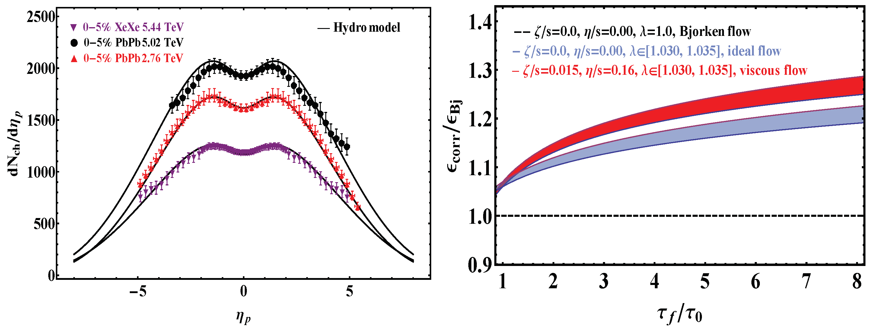
2. Pseudorapidity Distribution from Hydrodynamics
3. Relationship between the Energy Density Estimation and Viscous Effect
4. Conclusions and Discussion
Author Contributions
Funding
Acknowledgments
Conflicts of Interest
References
- Bass, S.A.; Gyulassy, M.; Stöecker, H.; Greiner, W. Signatures of quark gluon plasma formation in high-energy heavy-ion collisions: A Critical review. J. Phys. G Nucl. Part. Phys. 1999, 25, R1–R57. [Google Scholar] [CrossRef]
- Gyulassy, M.; McLerran, L. New forms of QCD matter discovered at RHIC. Nucl. Phys. A 2005, 750, 30–63. [Google Scholar] [CrossRef]
- Hwa, R.C. Statistical Description of Hadron Constituents as a Basis for the Fluid Model of High-Energy Collisions. Phys. Rev. D 1974, 10, 2260. [Google Scholar] [CrossRef]
- Bjorken, J.D. Highly Relativistic Nucleus-Nucleus Collisions: The Central Rapidity Region. Phys. Rev. D 1983, 27, 140. [Google Scholar] [CrossRef]
- Gubser, S.S. Symmetry constraints on generalizations of Bjorken flow. Phys. Rev. D 2010, 82, 085027. [Google Scholar] [CrossRef]
- Csörgő, T.; Grassi, F.; Hama, Y.; Kodama, T. Simple solutions of relativistic hydrodynamics for longitudinally expanding systems. Acta Phys. Hung. A 2003, 21, 53–62. [Google Scholar] [CrossRef]
- Csörgő, T.; Csernai, L.P.; Hama, Y.; Kodama, T. Simple solutions of relativistic hydrodynamics for systems with ellipsoidal symmetry. Acta Phys. Hung. A 2004, 21, 73–84. [Google Scholar] [CrossRef]
- Csörgő, T.; Nagy, M.I.; Csanád, M. A New family of simple solutions of perfect fluid hydrodynamics. Phys. Lett. B 2008, 663, 306. [Google Scholar] [CrossRef]
- Nagy, M.I.; Csörgő, T.; Csanád, M. Detailed description of accelerating, simple solutions of relativistic perfect fluid hydrodynamics. Phys. Rev. C 2008, 77, 024908. [Google Scholar] [CrossRef]
- Csörgo, T.; Kasza, G.; Csanád, M.; Jiang, Z.F. New exact solutions of relativistic hydrodynamics for longitudinally expanding fireballs. Universe 2018, 4, 69. [Google Scholar] [CrossRef]
- Marrochio, H.; Noronha, J.; Denicol, G.S.; Luzum, M.; Jeon, S.; Gale, C. Solutions of Conformal Israel-Stewart Relativistic Viscous Fluid Dynamics. Phys. Rev. C 2015, 91, 051702. [Google Scholar] [CrossRef]
- Hatta, Y.; Noronha, J.; Xiao, B.-W. Exact analytical solutions of second-order conformal hydrodynamics. Phys. Rev. D 2014, 89, 051702. [Google Scholar] [CrossRef]
- Nopoush, M.; Ryblewski, R.; Strickland, M. Anisotropic hydrodynamics for conformal Gubser flow. Phys. Rev. D 2015, 91, 045007. [Google Scholar] [CrossRef]
- Csörgő, T.; Lorstad, B. Bose-Einstein correlations for three-dimensionally expanding, cylindrically symmetric, finite systems. Phys. Rev. C 1996, 54, 1390. [Google Scholar] [CrossRef]
- Jiang, Z.F.; Yang, C.B.; Ding, C.; Wu, X.-Y. Pseudo-rapidity distribution from a perturbative solution of viscous hydrodynamics for heavy ion collisions at RHIC and LHC. Chin. Phys. C 2018, 42, 123103. [Google Scholar] [CrossRef]
- Adam, J.; et al. [ALICE Collaboration]. Centrality evolution of the charged-particlepseudorapidity density over a broad pseudorapidity range in Pb-Pb collisions at TeV. Phys. Lett. B 2016, 754, 373–385. [Google Scholar] [CrossRef]
- Adam, J.; et al. [ALICE Collaboration]. Centrality dependence of the pseudorapidity density distribution for charged particles in Pb-Pb collisions at TeV. Phys. Lett. B 2016, 722, 567–577. [Google Scholar]
- Acharya, S.; et al. [ALICE Collaboration]. Centrality and pseudorapidity dependence of the charged-particle multiplicity density in Xe-Xe collisions at TeV. arXiv 2018, arXiv:1805.04432. [Google Scholar]
- Jiang, Z.-F.; Yang, C.B.; Csanád, M.; Csörgő, T. Accelerating hydrodynamic description of pseudorapidity density and the initial energy density in p+p, Cu + Cu, Au + Au, and Pb + Pb collisions at energies available at the BNL Relativistic Heavy Ion Collider and the CERN Large Hadron Collider. Phys. Rev. C 2018, 97, 064906. [Google Scholar]
- Muronga, A. Causal theories of dissipative relativistic fluid dynamics for nuclear collisions. Phys. Rev. C 2004, 69, 034904. [Google Scholar] [CrossRef]
- Romatschke, P. New Developments in Relativistic Viscous Hydrodynamics. Int. J. Mod. Phys. E 2010, 19, 1–53. [Google Scholar] [CrossRef]
- Song, H.; Bass, S.A.; Heinz, U.; Hirano, T.; Shen, C. 200 A GeV Au+Au collisions serve a nearly perfect quark-gluon liquid. Phys. Rev. Lett. 2012, 10, 192301. [Google Scholar]
- Meyer, H.B. Calculation of the bulk viscosity in SU(3) gluodynamics. Phys. Rev. Lett. 2008, 100, 162001. [Google Scholar] [CrossRef]
- Pang, L.-G.; Petersen, H.; Wang, X.-N. Pseudorapidity distribution and decorrelation of anisotropic flow within CLVisc hydrodynamics. Phys. Rev. C 2018, 97, 064918. [Google Scholar] [CrossRef]
- Jiang, Z.-F.; Csanád, M.; Kasza, G.; Yang, C.B.; Csörgő, T. Pseudorapidity and initial energy densities in p+p and heavy ion collisions at RHIC and LHC. arXiv 2018, arXiv:1806.05750. [Google Scholar] [CrossRef]

| System | |||||
|---|---|---|---|---|---|
| 2.76 TeV | Pb+Pb | 1615 ± 39.0 | 1.035 ± 0.003 | 1.225 ± 0.022 | 1.285 ± 0.022 |
| 5.02 TeV | Pb+Pb | 1929 ± 47.0 | 1.032 ± 0.002 | 1.204 ± 0.012 | 1.263 ± 0.015 |
| 5.44 TeV | Xe+Xe | 1167 ± 26.0 | 1.030 ± 0.003 | 1.190 ± 0.021 | 1.248 ± 0.022 |
© 2019 by the authors. Licensee MDPI, Basel, Switzerland. This article is an open access article distributed under the terms and conditions of the Creative Commons Attribution (CC BY) license (http://creativecommons.org/licenses/by/4.0/).
Share and Cite
Gong, X.-T.; Jiang, Z.-F.; She, D.; Yang, C.B. Viscous Hydrodynamic Description of the Pseudorapidity Density and Energy Density Estimation for Pb+Pb and Xe+Xe Collisions at the LHC. Universe 2019, 5, 112. https://doi.org/10.3390/universe5050112
Gong X-T, Jiang Z-F, She D, Yang CB. Viscous Hydrodynamic Description of the Pseudorapidity Density and Energy Density Estimation for Pb+Pb and Xe+Xe Collisions at the LHC. Universe. 2019; 5(5):112. https://doi.org/10.3390/universe5050112
Chicago/Turabian StyleGong, Xiong-Tao, Ze-Fang Jiang, Duan She, and C. B. Yang. 2019. "Viscous Hydrodynamic Description of the Pseudorapidity Density and Energy Density Estimation for Pb+Pb and Xe+Xe Collisions at the LHC" Universe 5, no. 5: 112. https://doi.org/10.3390/universe5050112
APA StyleGong, X.-T., Jiang, Z.-F., She, D., & Yang, C. B. (2019). Viscous Hydrodynamic Description of the Pseudorapidity Density and Energy Density Estimation for Pb+Pb and Xe+Xe Collisions at the LHC. Universe, 5(5), 112. https://doi.org/10.3390/universe5050112