Article

Greybody Factors for Schwarzschild Black Holes: Path-Ordered Exponentials and Product Integrals

School of Mathematics and Statistics, Victoria University of Wellington, PO Box 600, Wellington 6140, New Zealand
*
Author to whom correspondence should be addressed.
Current address: Perimeter Institute, Waterloo, ON N2L 2Y5, Canada; [email protected] and Department of Physics and Astronomy, University of Waterloo, Waterloo, ON N2L 3G1, Canada.
Universe 2018, 4(9), 93; https://doi.org/10.3390/universe4090093
Submission received: 14 August 2018 / Revised: 28 August 2018 / Accepted: 28 August 2018 / Published: 3 September 2018
(This article belongs to the Collection Open Questions in Black Hole Physics)

Abstract

:
In earlier work concerning the sparsity of the Hawking flux, we found it necessary to re-examine what is known regarding the greybody factors of black holes, with a view to extending and expanding on some old results from the 1970s. Focusing specifically on Schwarzschild black holes, we have re-calculated and re-assessed the greybody factors using a path-ordered-exponential approach, a technique which has the virtue of providing a pedagogically useful semi-explicit formula for the relevant Bogoliubov coefficients. These path-ordered-exponentials, being based on a variant of the “transfer matrix” formalism, are closely related to so-called “product integrals”, leading to quite straightforward and direct numerical evaluation, while side-stepping any need for numerically solving the relevant ordinary differential equations. Furthermore, while considerable analytic information is already available regarding both the high-frequency and low-frequency asymptotics of these greybody factors, numerical approaches seem better adapted to finding suitable “global models” for these greybody factors in the intermediate frequency regime, where most of the Hawking flux is actually concentrated. Working in a more general context, these path-ordered-exponential techniques are also likely to be of interest for generic barrier-penetration problems.

1. Introduction

In earlier work [1,2] on the sparsity of the Hawking flux, the present authors (and two others) found it necessary to numerically evaluate certain greybody factors for the transmission of mass-less bosons through the Regge–Wheeler potential—the combined gravitational and angular momentum potential barrier surrounding a Schwarzschild black hole. While significant work on this topic dates back to the mid-1970’s, see in particular References [3,4,5,6], we felt it useful to completely re-assess the situation in terms of a radically different formalism using path-ordered matrix exponentials [7,8,9], a formalism closely related both to “transfer matrices”, and to the so-called “product integral” [10,11,12,13,14]. One of the virtues of using path-ordered matrix exponentials is that it gives a pedagogically useful semi-explicit expression for the Bogoliubov coefficients, and so gives a somewhat deeper analytic understanding of the transmission and reflection probabilities [15,16,17]. Path-ordered matrix exponentials are also relatively simple to evaluate numerically, and to obtain the transmission probabilities one never actually has to solve a numerical differential equation, one just performs a numerical integral.
In counterpoint, there has also been a lot of work done on both low-frequency and high-frequency limits for the greybody factors. (See for instance references [3,18] for low-frequency limits, and references [19,20,21] for high-frequency limits.) Information at intermediate frequencies is significantly harder to come by, and we shall use our numerical insights to try to develop some semi-analytic understanding of the intermediate frequency regime. Specifically, we shall build some models for the emission spectrum that use a small number of parameters to provide a good global fit to the Hawking spectrum.
We emphasize that while in the current article we are specifically interested in black hole physics, the path-ordered matrix exponential formalism [7,8,9] is a general-purpose tool, of wide applicability to both barrier penetration and scattering processes.

2. Strategy

Consider a Schrödinger-like scattering problem of the form:
d 2 d x 2 ψ ( x ) + V ( x ) ψ ( x ) = ω 2 ψ ( x ) ; V ( x ± ) 0 .
For any such problem, as long as V ( x ) is integrable (we do not, at this stage, need to impose any differentiability or continuity assumptions) and ω is real, one can define Bogoliubov coefficients relating the asymptotic left and right free-particle states, and derive the exact path-ordered-exponential result [7]:
α ( ω ) β * ( ω ) β ( ω ) α * ( ω ) = P exp i 2 ω + V ( x ) 1 e 2 i ω x e 2 i ω x 1 d x .
A brief sketch of the derivation is given in Appendix A; see also Reference [7] for full details. This result, and various generalizations and modifications thereof, has been used in a number of subsequent articles to develop quite general and useful bounds on transmission probabilities, both generic and black hole specific. See for instance References [7,8,9], additional formal developments in References [15,16,17], and some applications in References [22,23,24]. The key point is that the Bogoliubov coefficients satisfy | α ( ω ) | 2 | β ( ω ) | 2 = 1 , and that the transmission probability is simply:
T ( ω ) = 1 α ( ω ) α * ( ω ) = 1 | α ( ω ) | 2 .
In the current article, instead of looking for bounds, we shall instead use this path-ordered exponential technique as a basis for numerically calculating greybody factors for the Schwarzschild black hole. The key steps are to replace the position x by the tortoise coordinate r * , and to replace V ( x ) by the Regge–Wheeler potential [9,25]. Some formal developments are relegated to Appendix B.

3. Path-Ordered-Exponentials and the Product Calculus

Fundamentally, the primary definition of the path ordered exponential for a real or complex valued m × m matrix function A ( x ) from some initial point x i to some final point x f , is simply:
P exp x i x f A ( x ) d x lim N k = 0 N 1 exp A ( x k * ) Δ x k .
Here, closely following the usual technical construction of the Riemann integral, we shall take the “evaluation points” x k * [ x k , x k + 1 ] to be a tag of some partition { x k } k = 0 N of the interval [ x i , x f ] = [ x 0 , x N ] , with individual widths Δ x k = ( x k + 1 x k ) , and with the mesh ( D = max Δ x k ) going to zero in the limit N .
This definition of the path ordered exponential is completely equivalent to (a matrix-valued, non-commutative) definition of the so-called “product integral” [10,11,12,13,14]. The product calculus is exactly an alternative modified notion of calculus based on infinitesimal products and divisions, (recall that ordinary calculus is based on infinitesimal sums and subtractions).
In the language of the product calculus Equation (4) becomes:
P exp x i x f A ( x ) d x = x i x f I + A ( x ) d x .
Here, the product integral is defined as [10,11,12,13,14]:
x i x f I + A ( x ) d x lim N k = 0 N 1 I + A ( x k * ) Δ x k ,
with the partition { x k } k = 0 N of [ x i , x f ] = [ x 0 , x N ] , the tag x k * , the width Δ x k , and the mesh D, again being defined as before. The equivalence of the two definitions given in Equations (4) and (6) can be deduced by noting that all the second order or higher times in exp ( A ( x k * ) Δ x k ) go to zero in the limit D 0 [13]. Note that if the matrix A ( x ) happens to be nilpotent of degree two so that A ( x ) 2 = 0 , (which is quite often the case), then we have the exact result that exp A ( x k * ) Δ x k = I + A ( x k * ) Δ x k , and so the equality holds even before the limit of vanishing mesh is taken. See, for instance, References [13,14] for an overview of the product calculus. The following results for the product integral [10,11,12,13,14] should be especially noted:
  • If a b ( I + A d x ) exists, then A ( x ) is bounded on [ a , b ] .
  • If a b ( I + A d x ) exists, and a u < v b , then u v ( I + A d x ) exists.
  • If a < b < c , and both a b ( I + A d x ) and b c ( I + A d x ) exist, then:
    a c ( I + A d x ) = a b ( I + A d x ) × b c ( I + A d x ) .
  • a b ( I + A d x ) exists if and only if a b A d x exists (in the sense of the Riemann integral).
  • If a b ( I + A d x ) exists, then:
    a b ( I + A d x ) = I + a b A ( x 1 ) d x 1 + a b a x 1 A ( x 1 ) A ( x 2 ) d x 2 d x 1 + a b a x 1 a x 2 A ( x 1 ) A ( x 2 ) A ( x 3 ) d x 3 d x 2 d x 1 + . . .
Equation (8) is commonly known in the mathematics community as the Peano series, and in the physics community as the Dyson series. There are also alternative expansions available in terms of the Magnus series and/or Fer series that might sometimes be useful, but we shall not explore such options here. This Dyson series is the physics community’s standard method for approximating path ordered exponentials. Using the path-ordering operator P , Equation (8) can be re-written as:
a b ( I + A d x ) = n = 0 1 n ! a b d x 1 a b d x 2 a b d x n P A ( x 1 ) A ( x 2 ) A ( x n ) ,
where now
P A ( x 1 ) A ( x 2 ) A ( x n ) = A ( x σ ( 1 ) ) A ( x σ ( 2 ) ) A ( x σ ( n ) ) ,
with σ ( i ) being any permutation such that x σ ( 1 ) x σ ( 2 ) x σ ( n ) . For example
P A ( x 1 ) A ( x 2 ) = Θ ( x 1 x 2 ) A ( x 1 ) A ( x 2 ) + Θ ( x 2 x 1 ) A ( x 2 ) A ( x 1 ) ,
where Θ ( x ) is the Heaviside step function.
When written in the form of Equation (5), the transfer matrix of Equation (2) is particularly simple to evaluate numerically.
Defining
A ( x k ) i 2 ω V ( x k ) 1 e 2 i ω x k e 2 i ω x k 1 ,
we note A ( x k ) 2 = 0 ; so A ( x i ) is is indeed nilpotent of degree two. The transfer matrix can be compactly written as:
E ( x i , x f ) = lim N k = 1 N I + A ( x k ) h = lim N I + A ( x N 1 ) h I + A ( x 2 ) h I + A ( x 1 ) h .
Here, h = ( x f x i ) / N , and we have chosen the right-tagged equipartition x k = x i + k h . This naive expression is extremely easy to compute numerically; however much like a simple Riemann sum, convergence can sometimes be rather slow. That is, in terms of the underlying physics the discussion above is perfectly adequate, but simply to improve numerical convergence and stability a digression to considering the Helton–Stuckwisch algorithm is warranted.

4. Helton–Stuckwisch Algorithm

In order to improve convergence, Helton and Stuckwisch [11] introduce the equivalent of a product integral version of a higher-order Simpson rule. The Helton–Stuckwisch algorithm is based on summing a polynomial approximation which has absolute error bounded by H ( x i , x f ) h p . Here. H ( x i , x f ) is a bounded function determined by the matrix function A ( x ) and the interval [ x i , x f ] , and which is independent of the index p; where p is the order of the polynomial approximation. It is at this stage that one has to make some smoothness assumptions. To ensure p-th order convergence, the p-th order Helton–Stuckwisch algorithm requires the matrix function A ( x ) to be ( p + 1 ) -times continuously differentiable.
A minor technical issue is that Helton and Stuckwisch use a definition of the product integral based on right hand multiplication, that is, the order of the products in Equation (6) is reversed. This can be related to the form in Equation (6) by noting that in the limit N ,
x i x f I + A ( x ) d x 1 = lim N I + A ( x N 1 ) h . . . I + A ( x 2 ) h I + A ( x 1 ) h 1 = lim N I + A ( x N 1 ) h . . . I + A ( x 2 ) h I + A ( x 1 ) h 1 = lim N I A ( x 1 ) h I A ( x 2 ) h . . . I A ( x N 1 ) h .
Thus by sending A ( x i ) A ( x i ) and using the approximation in Reference [11], we obtain the inverse of the product integral we set out to calculate. Since the Bogoliubov matrix satisfies:
α β * β α * 1 = α * β * β α ,
we see that there is no loss of information; this method lends itself very well to finding the transmission probabilities.
The specific 5th-order approximation Helton and Stuckwisch introduce is [11]:
k = 1 N I + h / 90 7 A 0 + 32 A 1 + 12 A 2 + 32 A 3 + 7 A 4 + ( h 2 / 90 ) ( 8 A 0 A 1 12 A 0 A 2 + 18 A 0 A 3 7 A 0 A 4 + 18 A 1 A 2 12 A 1 A 3 + 18 A 1 A 4 + 18 A 2 A 3 12 A 2 A 4 + 8 A 3 A 4 ) + ( h 3 / 60 ) ( 3 A 0 A 1 A 2 2 A 0 A 1 A 3 + 3 A 0 A 1 A 4 2 A 0 A 2 A 3 2 A 0 A 2 A 4 + 3 A 0 A 3 A 4 + 8 A 1 A 2 A 3 2 A 1 A 2 A 4 2 A 1 A 3 A 4 + 3 A 2 A 3 A 4 ) + ( h 4 / 120 ) 4 A 0 A 1 A 2 A 3 A 0 A 1 A 2 A 4 A 0 A 1 A 3 A 4 A 0 A 2 A 3 A 4 + 4 A 1 A 2 A 3 A 4 + ( h 5 / 120 ) A 0 A 1 A 2 A 3 A 4 A 5 .
Here, A j = A ( x k 1 + j h / 4 ) for j = 0 , 1 , 2 , 3 , 4 and k = 1 , 2 , , N .
This somewhat unwieldy expression can more compactly be rewritten as follows [11]:
k = 1 N I + ( 28 K 1 + 32 K 2 + 6 K 3 + 4 K 4 + K 5 ) / 360 .
Here
K 1 = h A 4 K 2 = h A 3 ( 4 I + K 1 ) K 3 = h A 2 [ 8 ( I K 1 ) + 3 K 2 ] K 4 = h A 1 [ 32 I + 18 K 1 + 3 h A 2 ( 6 I K 1 + K 2 ) 3 K 2 ] K 5 = h A 0 [ 28 ( I K 1 ) 3 h A 2 ( 16 I + 4 K 1 + K 2 ) + K 4 + 18 K 2 ] .
This numerical scheme will be our primary tool for actually evaluating greybody factors. We first tested our technique in two situations, the square-barrier potential and the delta-function potential, where exact analytic results are known. We thereby verified that the numerical integration adequately approximated the exact results (details mercifully suppressed), before turning to the Schwarzschild geometry and its associated Regge–Wheeler potential. We again emphasize that the primary importance of the Helton–Stuckwisch algorithm is simply to improve numerical stability and convergence; from a more formal perspective the simple Riemann sum is quite sufficient to completely understand the underlying basic physics.

5. Particle Emission from a Schwarzschild Black Hole

We now turn to the Regge–Wheeler potential, which is related to particle emission from black holes. In this situation there is no exact analytic expression for the transmission probability, neither by directly analyzing incoming and outgoing waves, nor via the product calculus method. Instead we must evaluate the Bogoliubov coefficients numerically. Oddly enough for this problem the exact wavefunctions are known in terms of Heun functions, though this observation is less useful than it might seem, simply because not enough is understood regarding the asymptotic behavior of these Heun functions. See References [26,27,28,29]. We shall work in “geometric units” where both G Newton 1 and c 1 .

5.1. Setup

The probability of emission (the greybody factors), of massless particles from a black hole can be found by analyzing the appropriate wave equation in curved spacetime. For example, for a scalar field ψ ( x ) one considers:
a a ψ = 0 ,
where a is the covariant derivative with the Christoffel connexion associated with the spacetime metric g a b . The probability of emission is related to the ratio of the amplitude of inward and outward radially traveling solutions to Equation (18) at spatial infinity. It can be shown, using separation of variables, that for a non charged, spherically symmetric (Schwarzschild) black hole of mass M, this reduces to finding the transmission probability for Equation (1) with the Regge–Wheeler potential (see Reference [25] and, for more recent background, Reference [9] and References therein):
V ( r * ) = 1 2 M r ( r * ) ( + 1 ) r ( r * ) 2 + ( 1 s 2 ) 2 M r ( r * ) 3 .
Here, r is the usual radial coordinate, and r * the so-called tortoise coordinate. They are explicitly related by:
r * ( r ) = r + 2 M ln r 2 M 1 ; r ( r * ) = 2 M 1 + W exp r * 2 M 1 ,
where W ( x ) is the Lambert W function [9,30,31,32].
In addition, is the principal angular momentum number, and s is the spin of the particle. s { 0 , 1 , 2 } for scalars, photons, and gravitons, respectively, and { s , s + 1 , } . There are 2 + 1 azimuthal modes for each principle angular momentum mode, , which in the case of spherical symmetry are equiprobable. The emission rate d N s ( ω ) / d t d ω gives the total probability for an emission, per unit time, per unit frequency, of a particle of spin s and frequency ω . It is given by the sum over the transmission probabilities T , s ( ω ) , (Equation (3)), for each principal and azimuthal angular momentum mode, multiplied by the probability for a particle to be in a given mode P , s ( ω ) . That is [3,33,34,35]:
d N s ( ω ) d t d ω = = s ( 2 + 1 ) T , s ( ω ) P , s ( ω ) ,
where for a Schwarzschild black hole and integer spin particles, the probability for the particle to be in a given mode is given by the Bose–Einstein distribution,
P , s ( ω ) = g 2 π 1 exp ( 8 π M ω ) 1 ,
and g is the number of polarizations for a given spin s. Equation (21) represents the rate of the emission of particles. Each particle carries one quantum of energy, ω , and so the energy emission is given by
d E s ( ω ) d t d ω = ω d N s ( ω ) d t d ω .
Another physically important quantity is the cross-section, σ ( ω ) , which represents an effective area that embodies the likelihood of a particle to be scattered, (i.e., deflected), by the black hole. This is intimately related to the probability of transmission through the potential barrier [3]
σ s ( ω ) = π ω 2 = s ( 2 + 1 ) T , s ( ω ) .
In the high frequency limit M ω 1 this approaches the classical geometric optics cross-section σ = 27 π M 2 [3]. This can now be used to define the dimensionless cross-section, S ( x ) , by
S ( x ) = σ ( x ) σ = 1 27 x 2 = s ( 2 + 1 ) T , s ( x ) ,
where x = M ω . Equation (25) can then be used to rewrite Equations (21) and (23) in dimensionless form,
M d E s ( x ) d t d ω = x d N s ( x ) d t d ω = g 2 π 27 x 3 S ( x ) exp ( 8 π x ) 1 .
Now the Regge–Wheeler potential is asymptotically zero at both ends, (that is, we have V ( r * ) 0 as r * ± ). So using Equation (3) the transmission probabilities can be calculated from the Bogoliubov coefficients, as given in Equation (2). In this case (now working in terms of the dimensionless variables u * = r * / 2 M and u ( u * ) = r ( u * ) / 2 M ), the transfer matrix becomes
α β * β α * = P exp i 4 x + V ( u * ) 1 exp ( 4 i x u * ) exp ( 4 i x u * ) 1 d u * .
Here, the potential is now
V ( u * ) = 1 1 u ( u * ) ( + 1 ) u ( u * ) 2 + ( 1 s 2 ) u ( u * ) 3 .
In the product calculus formalism this leads to
α β * β α * = + ( I + A ( u * ) d u * ) ,
where
A ( u * ) i 4 x V ( u * ) 1 e 4 i x u * e 4 i x u * 1 .
It is also possible to do a little further pre-processing by changing variables in the path-ordered integral. This might somewhat help analytic insight, but does not seem to improve the numerics. See Appendix B for details.

5.2. Numerics

The calculation for the transmission probabilities for the Regge–Wheeler potential was numerically implemented in Python by using the polynomial approximation of Equation (17). The integration region [ , + ] was approximated by the finite range [ 50 , 350 ] , which was found to introduce an absolute error of at worst O ( 10 9 ) . Numerical convergence tests for the product integrals are summarized in Figure 1.
Figure 2 shows the transmission probability for each of the scalar, photon, and graviton cases. It can be seen that the s = 0 case has transmission at the lowest frequencies, and that in each case larger values require higher frequencies before there is any transmission through the barrier. Furthermore for each eventually (at high enough frequencies) there is complete transmission through the barrier. This can be interpreted physically by observing that the potential V ( r * ) is lowest for the = 0 = s case and, as such, less energy (i.e. lower frequency) is required to pass through the barrier. For larger and s values the potential is higher, and so more energy is required. Eventually, any particle species in any mode will have enough energy to completely pass through the barrier, i.e. T , s ( x ) 1 as x .
These greybody factors (for the Regge–Wheeler potential in Schwarzschild spacetime) exhibit very strong similarities and relatively minor differences. The greybody factors almost seem to be translations of one another, and all appear to be similar to suitably shifted hyperbolic tangent functions. See Figure 3. We shall discuss the implications of this observation more fully in the subsequent section on “modeling”.
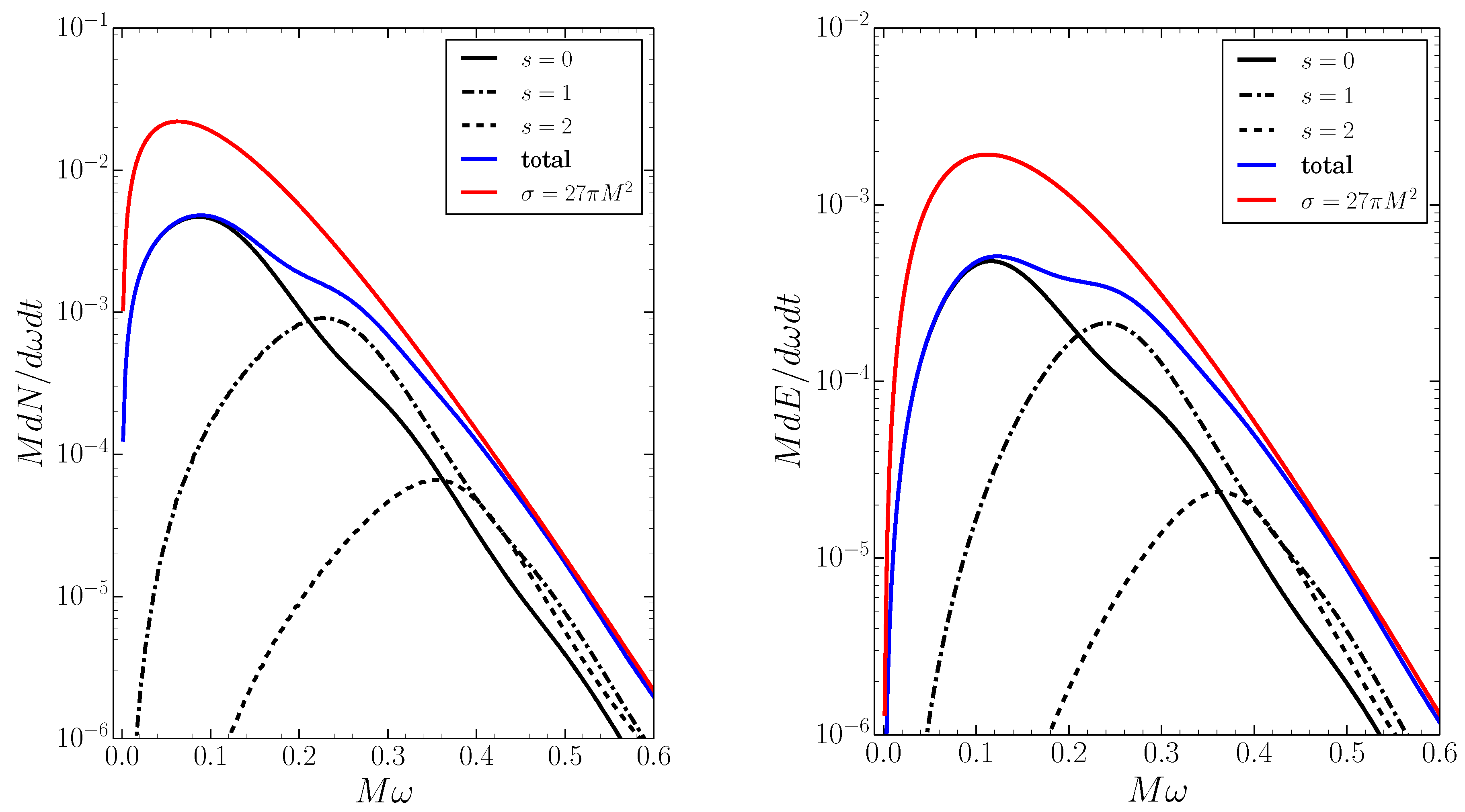
Figure 4 shows plots of both the number and energy emissions rates, Equations (21) and (23). It can be seen that for x 0.6 , the emission rate rapidly becomes negligible, exponentially decaying to zero. The emission of particles is dominated by scalars, and the rate reduces with increasing spin. This can be understood from Figure 2, in which it can be seen that for lower spin s the transmission probabilities become significant at smaller x; this coincides with the peak in the probability spectrum P , s ( x ) . For spin s, most of the interesting physics is concentrated in the range x [ 0 , ( s + 1 ) / 27 ] , whereas for total emissivity most of the interesting physics is concentrated in the range x [ 0 , 1 / 27 ] .
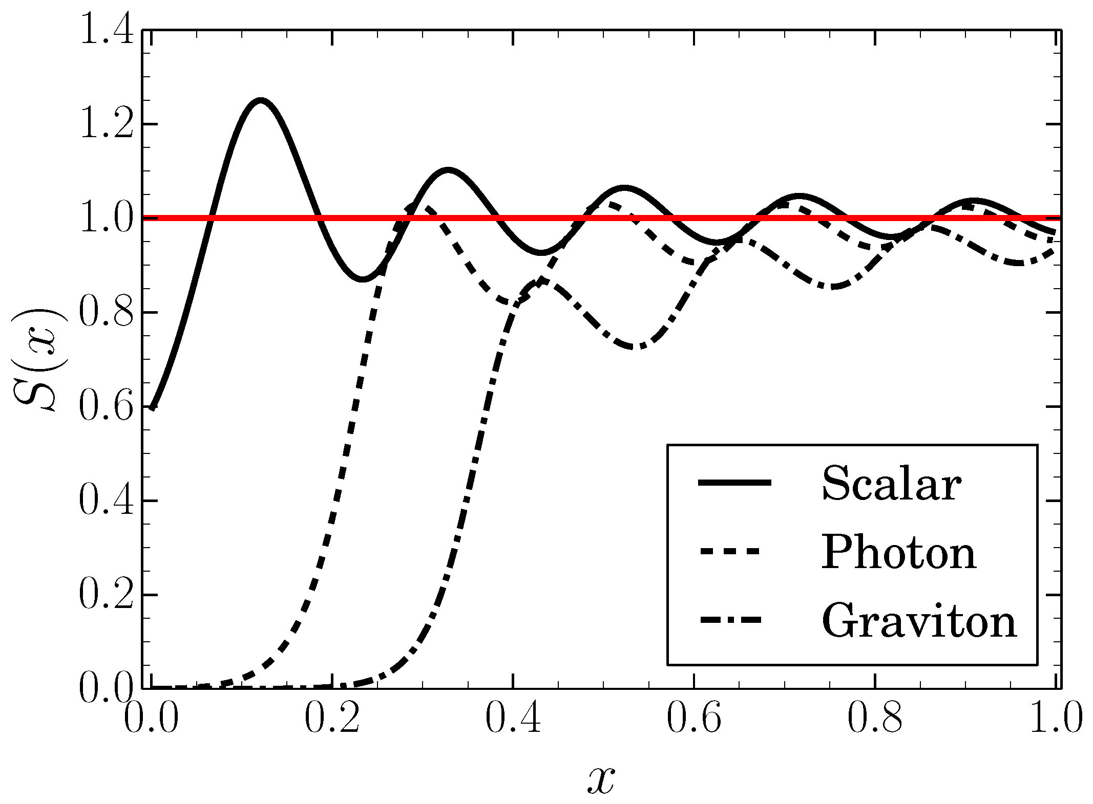
Finally, Figure 5 shows a numerical plot of the dimensionless cross-section, for each species of particle. As x increases, the cross-section approaches the geometric optics limit, i.e. S ( x ) 1 . This happens more quickly for lower spins. Each species also exhibits oscillations which are due to the transmission probabilities becoming appreciable for increasing values, weighted by the 2 + 1 factor.

5.3. Modeling the Greybody Factors and Cross-Section

Given the numerical data and in view of other information we have available, to what extent can we characterize and model the most salient features of the greybody factors? In the low-frequency limit, we know that [3,18]:
T , s ( ω ) C , s x 2 + 2 ; with C , s = 2 2 + 2 ( s ) ! ! ( + s ) ! ( 2 ) ! ( 2 + 1 ) ! 2 .
At high frequencies, we know that (see particularly the discussion by Sanchez [19,20,21]):
T , 0 ( x ) 1 1 + exp ( 2 + 1 ) π 1 27 x 2 ( + 1 2 ) 2 ; ( x 1 ; 1 ) .
Unfortunately this conveys relatively little information beyond the fact that T ( x ) 1 exponentially rapidly as x . At intermediate frequencies, rather little qualitative or quantitative information regarding the greybody factors is available. In contrast, for the dimensionless (scalar) cross section S ( x ) , more is known. At intermediate/high frequencies, Sanchez gives the equivalent of [19,20,21]:
S s = 0 ( x ) 1 32 27 sin 2 π 27 x 2 π 27 x ; x 1 27 .
However, inspection of Figure 4 shows that the bulk of the total emission spectrum is concentrated in the range x [ 0 , 1 / 27 ] , where this is not all that good an approximation. In fact, the Sanchez approximation predicts a negative cross section S s = 0 ( 0 ) < 0 at x = 0 . In view of our numerical calculations above, can we now do something better?

5.3.1. Model 0

An extremely simple toy model that captures most (but not all) of the relevant physics, is to use a simple sigmoid function and take
T model 0 ( x ) = 1 1 + exp w , s [ x x , s * ] = 1 2 1 + tanh w , s 2 x x , s * .
The parameter w , s controls the (inverse) width of the transition zone from zero to one, and inspection of Figure 2 and Figure 3 indicates that the transition zone is close to 1 / 27 wide for all spins and angular momenta. This corresponds to w , s 27 .
The parameter x , s * controls the location of the transition zone from 0 to 1. For any x, only those modes with x , s * < x contribute appreciably to the sum in the dimensionless cross section S ( x ) . In fact, a very crude approximation is
S ( x ) < max ( x ) ( 2 + 1 ) 27 x 2 = max ( x ) 2 27 x 2 ; max ( x ) = max { : x , s * < x } .
However, S ( x ) 1 asymptotically, so max ( x ) 27 x , which can be inverted to yield
x , s * 27 as .
This observation explains why the transition zones, as displayed in Figure 2 and Figure 3, are roughly equally spaced, and explains the specific value of the spacing. In fact, inspection of Figure 2 and Figure 3 indicates that a tolerable approximation for all is
x , s * + 1 2 27 .

5.3.2. Model 1

Thus, with the specific values for the parameters deduced above, our simple toy model becomes
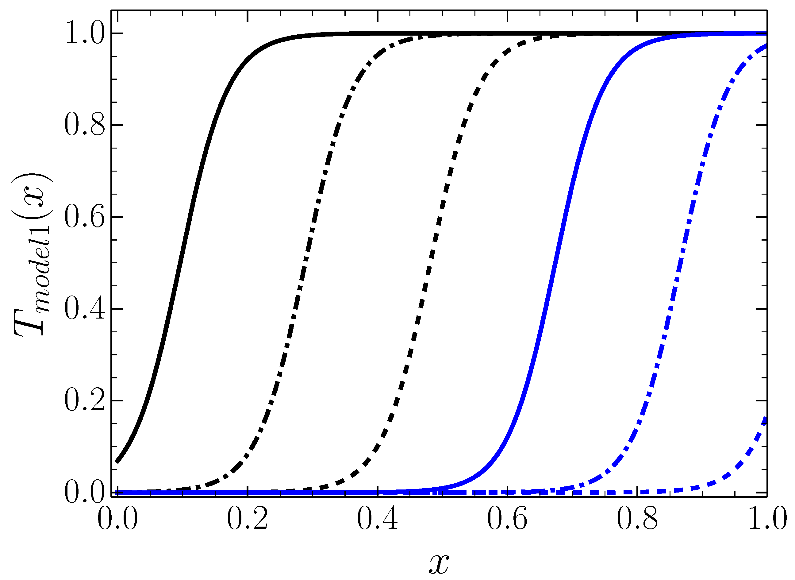
T model 1 ( x ) = 1 1 + exp 27 x 1 27 + 1 2 = 1 2 1 + tanh 27 2 x 1 27 + 1 2 .
See Figure 6, and compare this simple model with Figure 2 and Figure 3.

5.3.3. Model 2

The major weakness of this simple sigmoid model is the behavior as x 0 , where the non-zero limiting values of the greybody factors, T ( x 0 ) 0 , naively lead to an infinite cross section, S ( x 0 ) . The known x 0 behavior suggests we instead take something such as:
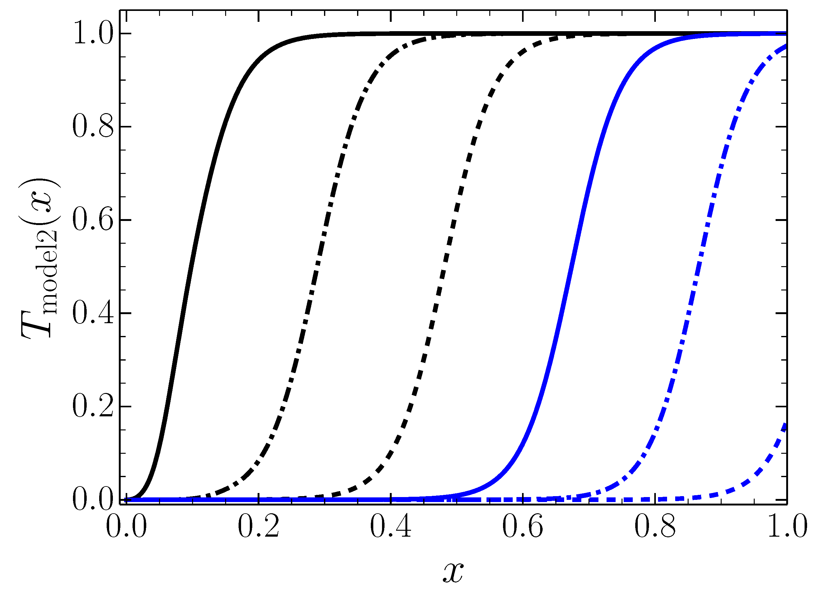
T model 2 ( x ) = tanh C , s x 2 + 2 1 + exp 27 + 1 2 1 + exp 27 x 1 27 + 1 2 .
Note this improved model simultaneously gives both the correct small x behavior, ( C , s x 2 + 2 ), the correct large x behavior ( T 1 ), and appropriate spacing and width for the transition zones, so S ( x ) 1 , as required. See Figure 7, and compare this simple model with Figure 2 and Figure 3. The corresponding cross sections are still not so good a fit at intermediate x. The locations of the peaks is fine, but the height of the first peak in S ( x ) is overestimated by some 75%.
In an attempt to further improve the model, one thing we looked at was the location and width of the transition zones. For the scalar case we found that
x , s = 0 * 1 27 + 1 2 + 1 16 ( + 1 2 )
gave a slightly better estimate for the location of the transition zones (presumably these are the first three terms of an asymptotic expansion). We also found it advantageous to artificially adjust the width parameter w , s 33 . Finally we tweaked the low-x behavior by noting that [ tanh ( z 1 n ) ] n tanh z at low z, while still approaching unity at large z, and chose n = 3 as a good fit.

5.3.4. Model 3

With these modifications in place we now have
T model 3 ( x ) = tanh C , s x 2 + 2 1 + exp 33 27 [ + 1 2 + 1 16 ( + 1 2 ) 1 / 3 3 1 + exp 33 x 1 27 + 1 2 + 1 16 ( + 1 2 ) .
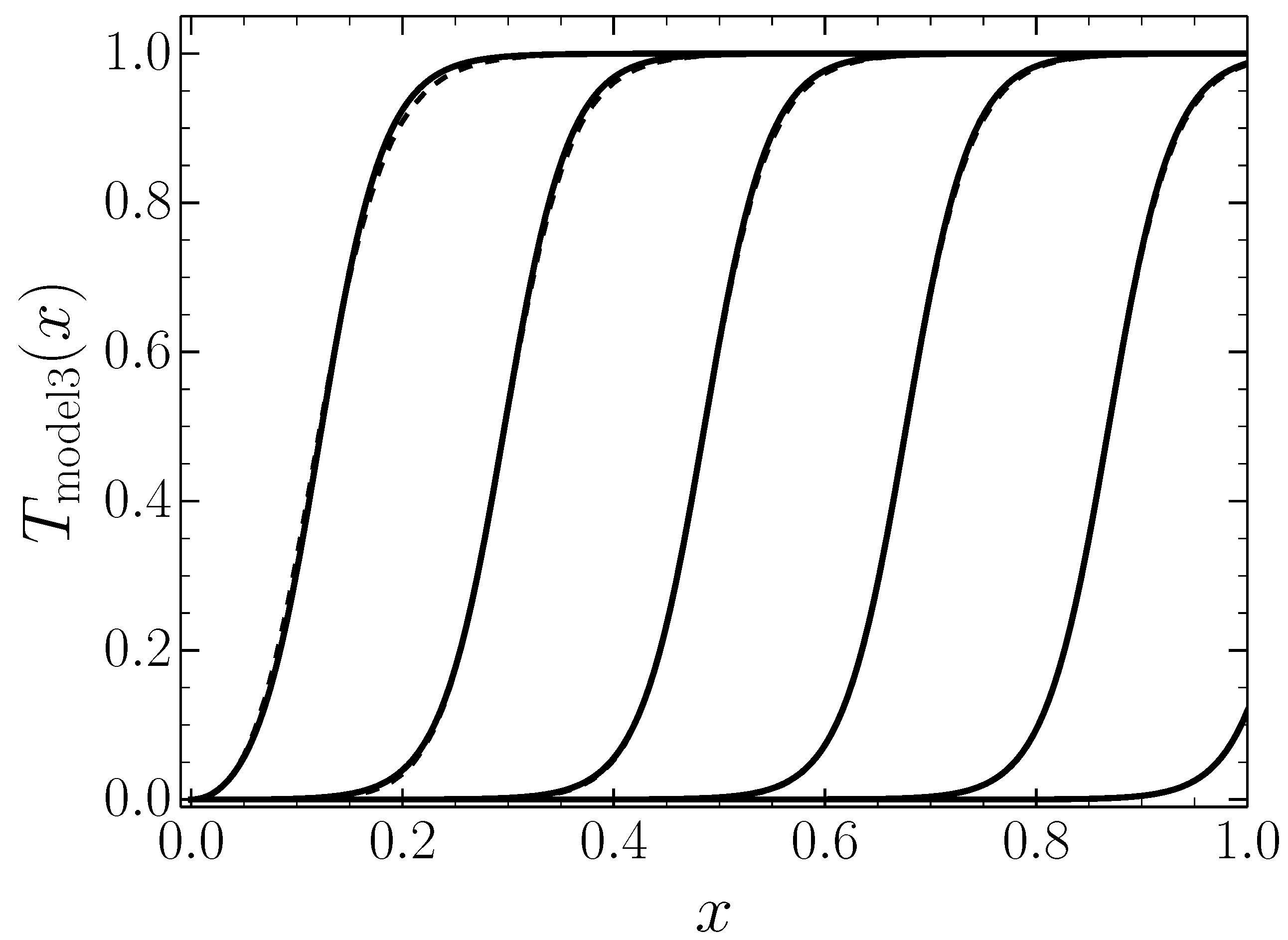
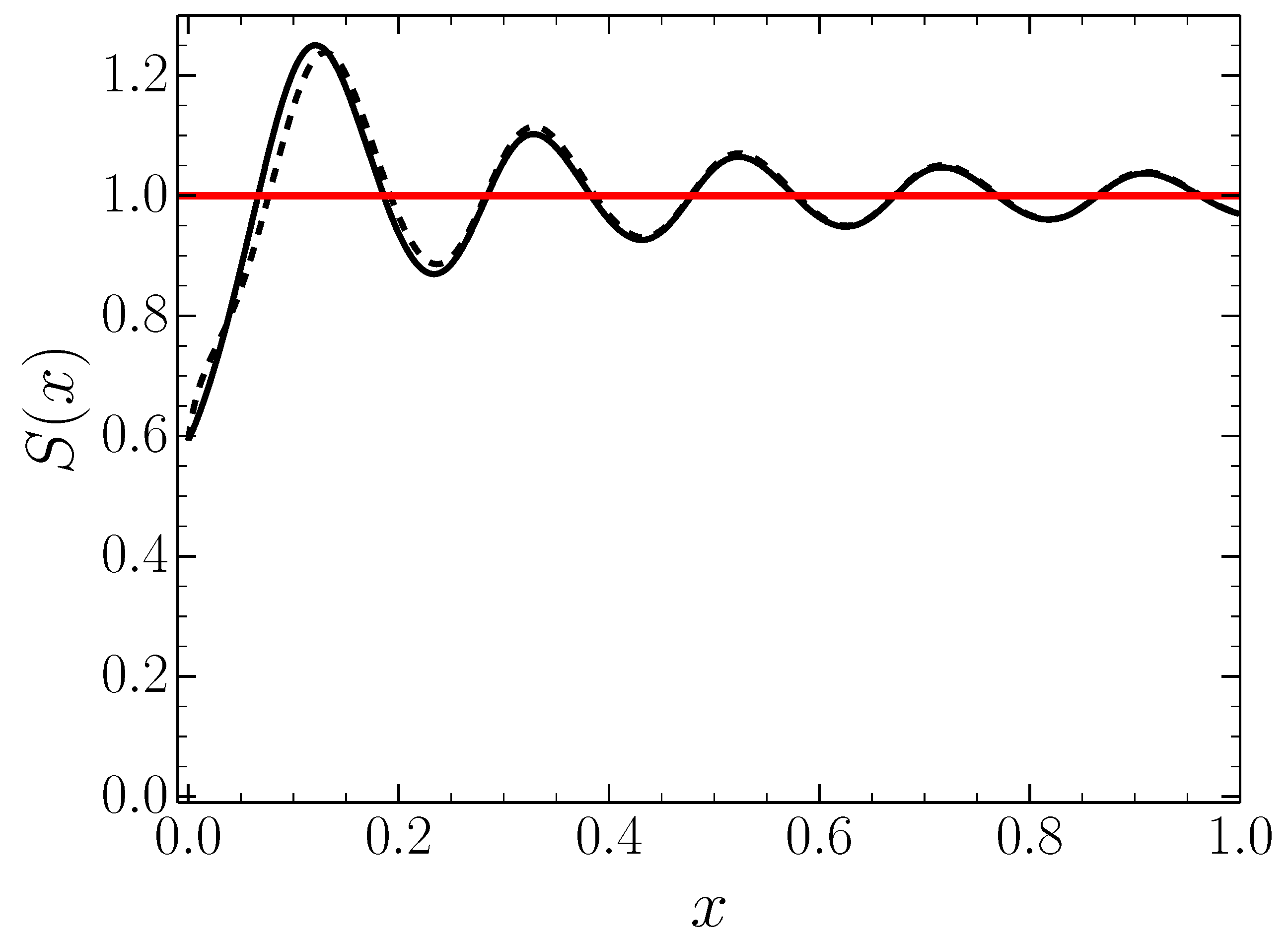
This gives a remarkably good fit to the (scalar) greybody factors and cross section. See Figure 8 and Figure 9. While it must be admitted that the model appears complicated, there are actually only three free parameters, the exponent 3 we have used in the tanh, the width parameter w , s 33 , and the shift in the location of the switchovers. The other parameters, such as C , s , the asymptotic location of the switchovers, the presence of the number 27, are fixed by the known asymptotic behavior of the greybody factors and cross section. Overall, this is a quite acceptable three-parameter fit, both to the scalar greybody factors and to the scalar cross section.
Fits to s = 1 and s = 2 could be developed along similar lines, by tweaking the exponent n in the tanh, the width parameter w , s , and the shift in the location of the switchovers. In the interests of brevity we restrict attention to the scalar case.

5.4. Directly Modeling the Cross Section

In counterpoint, we have also looked at the possibility of improving the Sanchez approximation directly (without explicitly worrying about the underlying greybody factors). The best we have been able to come up with is:
S ( x ) 1 32 27 sin 2 π 27 x 2 π 27 x + 32 27 11 27 exp 27 x 2 sin 3 2 π 27 x 3 2 π 27 x .
See Figure 10. The 32 / 27 is part of the original Sanchez approximation, and consequently the factor { 32 / 27 11 / 27 } is not a free parameter, as it is fixed by the known behavior at x = 0 : S ( 0 ) = 16 / 27 . Therefore there are only two free parameters: The 27 in the Gaussian, and the 3 2 π 27 were put in by hand, purely for observational reasons. We know of no good analytic reason for choosing such numbers, but the outcome is impressive. Overall, this is a quite acceptable two-parameter fit.
Décanini, Folacci, and Rafaelli [36] and Décanini, Esposito-Farese and Folacci [37] argue on semi-analytic grounds that the 32 / 27 , (which Sanchez obtains on purely numerical grounds), should more properly be replaced by 8 π e π . Numerically and visually these two options are indistinguishable. Fits to s = 1 and s = 2 could be developed along similar lines, by tweaking the width and oscillations of the subdominant term. In the interests of brevity we restrict attention to the scalar case.

6. Discussion

So what have we learned?
  • Path-ordered exponentials (transfer matrices, product integrals) are an effective way of first analytically expressing the Bogoliubov coefficients associated with a scattering problem, and second, can then be turned into an efficient algorithm for numerically calculating the Bogoliubov coefficients when the underlying problem is not analytically solvable. This observation is generic, not black-hole specific.
  • The path-ordered exponential formalism is the only way we know of to write down a more or less explicit formula for the Bogoliubov coefficients (and hence the transmission and reflection amplitudes) associated with a scattering problem.
  • Turning specifically to the Regge–Wheeler equation for the Schwarzschild black hole, the product integral (specifically the 5th order Helton–Stuckwisch algorithm, effectively a higher-order Simpson rule for product integrals), allowed us to quickly and efficiently calculate numerical greybody factors, which we then compared to older extant data from the 1970’s and also used in our own recent work on the sparsity of the Hawking flux. Perhaps more interestingly, once one has enough easily manipulable data on hand, it becomes feasible to undertake some semi-analytic model building to explore the structural details of the greybody factors.
  • The three-parameter fit we obtained to the (scalar) greybody factors seems quite good; likewise the two-parameter fit we obtained to the (scalar) cross section seems quite good.
  • These ideas could easily be extended to Reissner–Nordström, Kerr, and Kerr–Newman black holes, and, via the Teukolsky master equation, to higher spins. Generic “dirty” black holes (black holes surrounded by matter fields) can also be dealt with as soon as one derives a suitably generalized Regge–Wheeler equation.
We hope that these observations may be of wider interest, both in a general scattering context, and for black hole specific calculations.

Author Contributions

Formal analysis, F.G. and M.V.; Software, F.G.; Writing—original draft, F.G. and M.V.; Writing—review & editing, F.G. and M.V.

Funding

This research was funded by the Marsden Fund, and by a James Cook fellowship, both administered by the Royal Society of New Zealand. F.G. was also supported via a Victoria University of Wellington MSc scholarship.

Conflicts of Interest

The authors declare no conflict of interest.

Appendix A. Transmission and Reflection Coefficients

We wish to calculate the transmission and reflection coefficients for 1D Schrödinger-type equations
d 2 ψ d x 2 + V ( x ) ψ ( x ) = E ψ ( x ) ,
where the potential asymptotes to a constant,
lim x ± V ( x ) = V ± .
Later on, we will assume that V + = V , but in principle this is not required. In the two asymptotic regions there are two independent solutions [7]
ψ ± ± i ( x ) exp ( ± i ω ± x ) ω ± .
The ± i refers to right (left) moving modes, e i ω ± x ( e i ω ± x ) and ω ± = E V ± . To analyze the transmission and reflection coefficients, we consider the Jost solutions, J ± ( x ) , which are exact solutions to Equation (A1) satisfying
J ± ( x ± ) exp ( ± i ω ± x ) ω ± ,
and
J + ( x ) α exp ( + i ω x ) ω + β exp ( i ω x ) ω ,
J ( x + ) α * exp ( i ω + x ) ω + + β * exp ( + i ω + x ) ω + .
Here, α and β are the Bogoliubov coefficients, which are related to the reflection and transmission amplitudes by
r = β α ; t = 1 α ;
These Bogoliubov coefficients are for incoming/right moving waves which are partially scattered and transmitted by the potential V ( x ) . The reflection and transmission probabilities are then given by
R = | r | 2 ; T = | t | 2 .
That is, the probability for an incident particle to be reflected off or transmitted through the potential V ( x ) is given by R or T, respectively. Note that by definition, the sum of the probabilities for a particle to be reflected and transmitted must be unity:
R + T = 1 | α | 2 | β | 2 = 1 .
Now the second order Schrödinger Equation (A1) can be written as a Shabat–Zakharov system of coupled first order differential equations [8]. To do this, write the wave function as
ψ ( x ) = a ( x ) exp ( + i φ ) φ + b ( x ) exp ( i φ ) φ ,
where a ( x ) , b ( x ) are arbitrary functions, “local Bogoliubov coefficients”, and the auxiliary function, φ ( x ) , is chosen such that it has a non zero derivative and
φ ( x ) ω ± as x ± .
To reduce the number of degrees of freedom, we can impose the gauge condition,
d d x a φ e + i φ + d d x b φ e i φ = 0 .
We now define ω ( x ) 2 E V ( x ) and ρ φ + i [ ω 2 ( x ) ( φ ) 2 ] . Then, substitute Equation (A10) into Equation (A1). Using the gauge condition, Equation (A12), one obtains the following system of equations:
d d x a ( x ) b ( x ) = 1 2 φ i Im [ ρ ] ρ exp ( 2 i φ ) ρ * exp ( 2 i φ ) i Im [ ρ ] a ( x ) b ( x ) .
This has the formal solution [7],
a ( x f ) b ( x f ) = E ( x i , x f ) a ( x i ) b ( x i ) ,
in terms of a generalized position-dependent transfer matrix,
E ( x i , x f ) = P exp x i x f 1 2 φ i Im [ ρ ] ρ exp ( 2 i φ ) ρ * exp ( 2 i φ ) i Im [ ρ ] d x .
Here, “ P exp ” denotes a path ordered exponential operation. In the limit x i , x f + this becomes an exact expression for the Bogoliubov coefficients:
α β * β α * = E ( , ) = P exp + 1 2 φ i Im [ ρ ] ρ exp ( 2 i φ ) ρ * exp ( 2 i φ ) i Im [ ρ ] d x .
In the case V = V + , there is a natural choice for the auxiliary function. Simply take φ ( x ) ω x , where for simplicity we have written ω ω ± . With this choice, Equation (A15) can be seen to reduce to:
E ( x i , x f ) = P exp i 2 ω x i x f ( V ( x ) V ) 1 e 2 i ω x e 2 i ω x 1 d x ,
while Equation (A16) reduces to:
α β * β α * = P exp i 2 ω ( V ( x ) V ) 1 e 2 i ω x e 2 i ω x 1 d x .
Note the formalism is extremely general and flexible, and the current application to greybody factors is just one particular example of what can be done. See for instance References [7,8,9], related formal developments in References [15,16,17], and various applications in References [22,23,24].

Appendix B. Formal Developments for the Regge–Wheeler Equation

We are specifically interested in the problem
d 2 d r * 2 + ω 2 V ( r * ) ψ ( r * ) = 0 ,
where the Regge–Wheeler potential is
V ( r * ) = 1 2 M r ( + 1 ) r 2 + ( 1 s 2 ) 2 M r 3 ,
and the tortoise coordinate is
d r * d r = 1 1 2 M r .
We know
α β * β α * = P exp i 2 ω + V ( r * ) 1 e 2 i ω r * e 2 i ω r * 1 d r * .
Therefore, changing variables r * r , we have:
α β * β α * = P exp i 2 ω 2 M ( + 1 ) r 2 + ( 1 s 2 ) 2 M r 3 × 0 e 2 i ω r * ( r ) e 2 i ω r * ( r ) 0 d r .
But, writing the tortoise coordinate r * in terms of the r coordinate
r * ( r ) = r + 2 M ln r 2 M 1 ,
so
e 2 i ω r * ( r ) = e 2 i ω r r 2 M 1 4 i ω M .
Therefore, somewhat more explicitly, we have:
α β * β α * = P exp i 2 ω 2 M ( + 1 ) r 2 + ( 1 s 2 ) 2 M r 3 × 1 e 2 i ω r r 2 M 1 4 i ω M e 2 i ω r r 2 M 1 4 i ω M 1 d r .
Now perform another change of variables (to make everything dimensionless):
x = ω M ; u = r 2 M ; 2 x u = ω r .
Then:
α β * β α * = P exp i 4 x 1 ( + 1 ) u 2 + ( 1 s 2 ) u 3 × 1 e 4 i x u u 1 4 i x e 4 i x u u 1 4 i x 1 d u .
Finally, set w = 1 / u so that:
α β * β α * = P exp i 4 x 0 1 ( + 1 ) + ( 1 s 2 ) w × 1 e 4 i x / w 1 w w 4 i x e 4 i x / w 1 w w 4 i x 1 d w .
The benefit of these transformations is that the integral now runs over a finite range; the disadvantage is the rapid oscillations near the endpoints. From a theoretician’s perspective, this is now probably the most explicit formulation of the problem one can realistically hope for.

References

  1. Gray, F.; Schuster, S.; Van-Brunt, A.; Visser, M. The Hawking cascade from a black hole is extremely sparse. Class. Quantum Gravity 2016, 33, 115003. [Google Scholar] [CrossRef] [Green Version]
  2. Visser, M.; Gray, F.; Schuster, S.; Van-Brunt, A. Sparsity of the Hawking flux. In Proceedings of the MG14 Meeting on General Relativity (2017), Rome, Italy, 12–18 July 2015; pp. 1724–1729. [Google Scholar]
  3. Page, D.N. Particle emission rates from a black hole. I: Massless particles from an uncharged, nonrotating hole. Phys. Rev. D 1976, 13, 198–206. [Google Scholar] [CrossRef]
  4. Page, D.N. Particle emission rates from a black hole. II: Massless particles from a rotating hole. Phys. Rev. D 1976, 14, 3260–3273. [Google Scholar] [CrossRef]
  5. Page, D.N. Particle emission rates from a black hole. III: Charged leptons from a nonrotating hole. Phys. Rev. D 1977, 16, 2402–2411. [Google Scholar] [CrossRef]
  6. Page, D.N. Accretion into and Emission from Black Holes. Ph.D. Thesis (Cal Tech 1978). Available online: http://thesis.library.caltech.edu/7179/ (accessed on 3 September 2018).
  7. Visser, M. Some general bounds for 1-D scattering. Phys. Rev. A 1999, 59, 427–438. [Google Scholar] [CrossRef]
  8. Boonserm, P.; Visser, M. Reformulating the Schrodinger equation as a Shabat–Zakharov system. J. Math. Phys. 2010, 51, 022105. [Google Scholar] [CrossRef]
  9. Boonserm, P.; Ngampitipan, T.; Visser, M. Regge–Wheeler equation, linear stability, and greybody factors for dirty black holes. Phys. Rev. D 2013, 88, 041502. [Google Scholar] [CrossRef]
  10. Helton, J.C. Product integrals and the solution of integral equations. Pac. J. Math. 1975, 58, 87–103. [Google Scholar] [CrossRef] [Green Version]
  11. Helton, J.; Stuckwisch, S. Numerical approximation of product integrals. J. Math. Anal. Appl. 1976, 56, 410–437. [Google Scholar] [CrossRef]
  12. Dollard, J.D.; Friedman, C.N. Product integration of measures and applications. J. Differ. Equ. 1979, 31, 418–464. [Google Scholar] [CrossRef]
  13. Dollard, J.; Friedman, C. Product Integration with Application to Differential Equations; Encyclopedia of Mathematics and Its Applications; Cambridge University Press: Cambridge, UK, 1984. [Google Scholar]
  14. Slavík, A. Product Integration, Its History and Applications; Dějiny Matematiky, Matfyzpress: Prague, Czech Republic, 2007. [Google Scholar]
  15. Boonserm, P.; Visser, M. Bounding the Bogoliubov coefficients. Ann. Phys. 2008, 323, 2779–2798. [Google Scholar] [CrossRef] [Green Version]
  16. Boonserm, P.; Visser, M. Transmission probabilities and the Miller-Good transformation. J. Phys. A 2009, 42, 045301. [Google Scholar] [CrossRef]
  17. Boonserm, P.; Visser, M. Analytic bounds on transmission probabilities. Ann. Phys. 2010, 325, 1328–1339. [Google Scholar] [CrossRef]
  18. Starobinsky, A.A.; Churilov, S.M. Amplification of electromagnetic and gravitational waves scattered by a rotating black hole. Sov. Phys. JETP 1974, 65, 1–5. [Google Scholar]
  19. Sanchez, N.G. Scattering of scalar waves from a Schwarzschild black hole. J. Math. Phys. 1976, 17, 688. [Google Scholar] [CrossRef]
  20. Sanchez, N.G. The Wave Scattering Theory and the Absorption Problem for a Black Hole. Phys. Rev. D 1977, 16, 937–945. [Google Scholar] [CrossRef]
  21. Sanchez, N.G. Elastic Scattering of Waves by a Black Hole. Phys. Rev. D 1978, 18, 1798–1804. [Google Scholar] [CrossRef]
  22. Boonserm, P.; Visser, M. Bounding the greybody factors for Schwarzschild black holes. Phys. Rev. D 2008, 78, 101502. [Google Scholar] [CrossRef]
  23. Boonserm, P.; Ngampitipan, T.; Visser, M. Bounding the greybody factors for scalar field excitations on the Kerr–Newman spacetime. J. High Energy Phys. 2014, 2014, 113. [Google Scholar] [CrossRef]
  24. Boonserm, P.; Chatrabhuti, A.; Ngampitipan, T.; Visser, M. Greybody factors for Myers–Perry black holes. J. Math. Phys. 2014, 55, 112502. [Google Scholar] [CrossRef] [Green Version]
  25. Regge, T.; Wheeler, J.A. Stability of a Schwarzschild singularity. Phys. Rev. 1957, 108, 1063–1069. [Google Scholar] [CrossRef]
  26. Hortacsu, M. Heun Functions and their uses in Physics. In Proceedings of the 13th Regional Conference on Mathematical Physics, Antalya, Turkey, 27–31 October 2010. [Google Scholar]
  27. Fiziev, P.P.; Staicova, D. Application of the confluent Heun functions for finding the quasinormal modes of nonrotating black holes. Phys. Rev. D 2011, 84, 127502. [Google Scholar] [CrossRef]
  28. Fiziev, P.P. Exact solutions of Regge–Wheeler equation. J. Phys. Conf. Ser. 2007, 66, 012016. [Google Scholar] [CrossRef]
  29. Sanchez, N.G. In the exact solutions of the Regge–Wheeler equation in the Schwarzschild black hole interior. arXiv, 2006; arXiv:gr-qc/0603003. [Google Scholar]
  30. Corless, R.M.; Gonnet, G.H.; Hare, D.E.G.; Jeffrey, D.J.; Knuth, D.E. On the Lambert W function. Adv. Comput. Math. 1996, 5, 329–359. [Google Scholar] [CrossRef]
  31. Valluri, S.R.; Jeffrey, D.J.; Corless, R.M. Some applications of the Lambert W function to physics. Can. J. Phys. 2000, 78, 823–831. [Google Scholar]
  32. Visser, M. Primes and the Lambert W function. Mathematics 2018, 6, 56. [Google Scholar] [CrossRef]
  33. Hawking, S.W. Particle Creation by Black Holes. Commun. Math. Phys. 1975, 43, 199–220. [Google Scholar] [CrossRef]
  34. Hawking, S.W. Black Holes and Thermodynamics. Phys. Rev. D 1976, 13, 191–197. [Google Scholar] [CrossRef]
  35. Hartle, J.B.; Hawking, S.W. Path Integral Derivation of Black Hole Radiance. Phys. Rev. D 1976, 13, 2188–2203. [Google Scholar] [CrossRef]
  36. Decanini, Y.; Folacci, A.; Raffaelli, B. Fine structure of high-energy absorption cross sections for black holes. Class. Quant. Grav. 2011, 28, 175021. [Google Scholar] [CrossRef]
  37. Décanini, Y.; Esposito-Farese, G.; Folacci, A. Universality of high-energy absorption cross sections for black holes. Phys. Rev. D 2011, 83, 044032. [Google Scholar] [CrossRef]
Figure 1. Regge–Wheeler for Schwarzschild: Convergence tests. Convergence rates of the numerical transmission probabilities T s , s ( x ) , (greybody factors), for (a) scalars, (b) photons, and (c) gravitons. Here, we have defined the relative error of the N-th approximation, (i.e. the N term approximation), as δ T s , s | T s , s ( N ) ( x ) T s , s ( N + 1 ) ( x ) | / T s , s ( N ) ( x ) .
Universe 04 00093 g001
Figure 2. Regge–Wheeler for Schwarzschild: Greybody factors. Plots of the transmission probabilities, T , s ( x ) , as a function of x = M ω for, (a) scalars, (b) photons, and (c) gravitons. The leftmost function on each plot corresponds to the = s transmission probability, increasing values occur to the right.
Universe 04 00093 g002
Figure 3. Regge–Wheeler for Schwarzschild: Superimposed greybody factors. Note the very strong similarities and relatively minor differences. The greybody factors almost seem to be translations of one another, and are very similar to suitably shifted hyperbolic tangent functions. The left hand Figure merely superimposes the greybody factors. The middle Figure translates the greybody factors to the left by ( s ) / 27 before superimposing them. The right hand Figure translates the greybody factors to the left by / 27 before superimposing them.
Universe 04 00093 g003
Figure 4. Regge–Wheeler for Schwarzschild: Number and energy spectra. Plots of the number (left) and energy (right) emission spectra for a Schwarzschild black hole, see Equations (21) and (23). Note the logarithmic scale. The emission spectrum is dominated by scalar particles, and emission rates decrease with increasing spin. The total emission rates (i.e. summing over all particle species) are indicated in blue and are bounded by the sums over the geometric optics limit, σ = 27 π M 2 , for each species (shown in red), and this limit is approached as M ω .
Universe 04 00093 g004
Figure 5. Regge–Wheeler for Schwarzschild: Dimensionless cross-sections. The dimensionless cross-section S ( x ) , see Equation (25), plotted for scalars, photons, and gravitons for a Schwarzschild black hole.
Universe 04 00093 g005
Figure 6. Regge–Wheeler for Schwarzschild: Scalar greybody factors. Toy model # 1, Equation (38), for the greybody factors. From left to right the curves correspond to = 0 to = 5 . Note the bad behavior at x = 0 , though other gross features of the numerically determined greybody factors are adequately represented.
Universe 04 00093 g006
Figure 7. Regge–Wheeler for Schwarzschild: Scalar greybody factors. Toy model # 2, Equation (39), for the greybody factors. From left to right the curves correspond to = 0 to = 5 . Note improved behavior at x = 0 .
Universe 04 00093 g007
Figure 8. Regge–Wheeler for Schwarzschild: Scalar greybody factors. Toy model # 3, Equation (41), for the scalar greybody factors compared to the numerical data. From left to right the curves correspond to = 0 to = 5 . Note the solid curves are the numerical data, while the dashed curves are from our model # 3. The curves are often indistinguishable to the naked eye.
Universe 04 00093 g008
Figure 9. Regge–Wheeler for Schwarzschild: Scalar cross section. Dimensionless (scalar) cross section derived from the toy model # 3, Equation (41), for scalar greybody factors. Note the solid curve is based on the numerical data, while the dashed curve is from our model # 3. The fit is generally quite good and the curves are often indistinguishable to the naked eye.
Universe 04 00093 g009
Figure 10. Regge–Wheeler for Schwarzschild: Modified Sanchez approximation. The dashed curve is the model, our Equation (42), the solid curve is the numerical data. The fit is generally quite good and the curves are often indistinguishable to the naked eye.
Universe 04 00093 g010