Article

On Maximal Homogeneous 3-Geometries and Their Visualization †

Department of Geometry, Institute of Mathematics, Budapest University of Technology and Economics, Budapest, P.O. Box: 91, H-1521, Hungary
*
Author to whom correspondence should be addressed.
Dedicated to the Memory of Professor István Lovas.
These authors contributed equally to this work.
Universe 2017, 3(4), 83; https://doi.org/10.3390/universe3040083
Submission received: 25 October 2017 / Revised: 20 November 2017 / Accepted: 22 November 2017 / Published: 4 December 2017

Abstract

:
The motivation for this talk and paper is related to the classification of the homogeneous simply connected maximal 3-geometries (the so-called Thurston geometries: E 3 , S 3 , H 3 , S 2 × R , H 2 × R , S L 2 R ˜ , Nil , and Sol ) and their applications in crystallography. The first author found in (Molnár 1997) (see also the more popular (Molnár et al. 2010; 2015) with co-author colleagues, together with more details) a unified projective interpretation for them in the sense of Felix Klein’s Erlangen Program: namely, each S of the above space geometries and its isometry group Isom ( S ) can be considered as a subspace of the projective 3-sphere: S P S 3 , where a special maximal group G = Isom ( S ) Coll ( P S 3 ) of collineations acts, leaving the above subspace S invariant. Vice-versa, we can start with the projective geometry, namely with the classification of Coll ( P S 3 ) through linear transforms of dual pairs of real 4-vector spaces ( V 4 , V 4 , R , ) = P S 3 (up to positive real multiplicative equivalence ∼) via Jordan normal forms. Then, we look for projective groups with 3 parameters, and with appropriate properties for convenient geometries described above and in this paper.

1. Introduction

Our intention is to investigate and visualize the possible projective transforms, not considered earlier, for 3-parameter transitive translations, the possible invariant projective polarities, the possible invariant Riemann metrics, etc. Bolyai–Lobachevsky hyperbolic geometry H 3 is a particular example. We hope that we get further geometries, or that new interesting problems will arise, in this manner. We conjecture that our experience space can wear the structure of these 8 Thurston geometries, in small size at certain physical circumstances.
First, we look for a 3-parameter fixed point free group of translations, simply transitive on a 3-subspace. For instance, think of the classical Euclidean geometry E 3 where the 4 × 4 matrix group (first in the E 3 column)
E 3 : 1 x y z 0 1 0 0 0 0 1 0 0 0 0 1 ; Nil : 1 x y z 0 1 0 1 2 y 0 0 1 1 2 x 0 0 0 1 1 x y z 0 1 0 0 0 0 1 x 0 0 0 1 1 x y z 0 1 z y 0 0 1 x 0 0 0 1 ;
S L 2 R ˜ : x 0 x 1 x 2 x 3 x 1 x 0 x 3 x 2 x 2 x 3 x 0 x 1 x 3 x 2 x 1 x 0 ; Sol : 1 x y z 0 e z 0 0 0 0 e z 0 0 0 0 1 1 u v w 0 cosh w sinh w 0 0 sinh w cosh w 0 0 0 0 1
describes first the translation that carries the origin ( 1 , 0 , 0 , 0 ) into ( 1 , x , y , z ) in the classical homogeneous coordinate system E 0 , E 1 , E 2 , E 3 . This group is simply transitive on points and fixed point free on the affine 3-subspace A 3 = P 3 \ e 0 , where P 3 is obtained from the projective sphere P S 3 by the identification of opposite points, as usual, and e 0 is the ideal plane described by the linear form e 0 of the dual basis ( e 0 , e 1 , e 2 , e 3 ) in V 4 to the vector basis ( e 0 , e 1 , e 2 , e 3 ) in V 4 , i.e., e i e j = δ i j (the Kronecker symbol). That means, we get the Cartesian coordinate tetrahedron (simplex), where e 0 describes the origin E 0 , incident to the side planes e 1 , e 2 , e 3 by the corresponding forms. The ideal plane e 0 is opposite to the origin, and contains the ideal points E 1 , E 2 , E 3 of the x , y , z axes, respectively. Then, we extend this translation group with all projective collineations, leaving invariant a projective polarity (or scalar product) of signature ( + , + , + , 0 ) , with unimodular linear transforms, as usual. Now, think of the “optimal” generalizations of this, as made in the papers [1,2,3,4,5,6,7] for the above Thurston geometries.
Then, come above other three Thurston geometries, as examples. The second example is Nil in 2 equivalent interpretations. The second variant is the classical Heisenberg group in our projective sense. Indeed, with our translation matrix we get
( 1 , a , b , c , ) ( T 2 ) = ( 1 , x + a , y + b , z + b x + c ) ,
as the (non-commutative) translate of an arbitrary point ( a , b , c ) , in affine sense. The third component shows some “twist” effect as a characteristic property of Nil . The first variant of Nil is our initiative:
( 1 , a , b , c , ) ( T 1 ) = ( 1 , x + a , y + b , z + 1 2 ( a y + b x ) + c ) .
Here, the commutator of the first two ( e 1 and e 2 ) translations will just be the third ( e 3 ) translation. The 4th Sol geometry above is also an affine metric space in A 3 with strange metrics [7]; we indicate another Sol interpretation as well. However, S L 2 R ˜ (in our interpretation) needs the projective embedding into P S 3 indeed, similarly as S 3 , H 3 , S 2 × R , H 2 × R (see [1,6] not detailed here).
Our intention is to investigate the other possible projective transforms, not considered previously, for 3-parameter transitive translations, the possible invariant projective polarities, the possible invariant Riemann metrics, etc. We hope that we get further geometries, or that new interesting problems, and applications will arise. First, to be modest, we can restrict ourselves to collineations, commuting with typical one-parameter groups. See Cases (i), (ii) and some others as follows. We have some seemingly new candidate groups, in similar notations as above, not pretending completeness yet:
( i ) : 1 x y z 0 1 x 0 0 0 1 0 0 0 0 1 ; ( ii ) : 1 x y z 0 1 x y 0 0 1 x 0 0 0 1 ; ( iii ) 1 x y z 0 1 x 0 0 0 1 x 0 0 0 1 ;
( iv ) 1 x y z 0 1 x 0 0 0 1 y 0 0 0 1 ; ( v ) : 1 x y z 0 1 z 0 0 0 1 y 0 0 0 1 ; ( vi ) : cos t sin t u v sin t cos t v u 0 0 cos t sin t 0 0 sin t cos t ;
( vii ) cos t sin t u v sin t cos t v u u v cos t sin t v u sin t cos t ; ( viii ) : cosh t sinh t u v sinh t cosh t v u u v cosh t sinh t v u sinh t cosh t ;
Cases (vii) and (viii) are probably equivalent to S L 2 R ˜ geometry as above.
As usual, in each case, we form the inverse matrix, and pull back the arc element, e.g., ( 0 , d x , d y , d z ) from ( 1 , x , y , z ) to the origin. Here, we choose the standard positive-definite Riemann metrics, so we get the arc-length-square in each point. Then the Levi–Civita connection with Christoffel symbols Γ i j k below leads to the well known differential equation system (of second order, ( ) derivatives by the arc length s) of geodesic curve ( u 1 = x , u 2 = y , u 3 = z , Einstein–Schouten index convention!):
Γ i j k = 1 2 ( g j l / u i + g i l / u j g i j / u l ) g l k ( u ) k + Γ i j k ( u ) i ( u ) j = 0 ,
with given initial values of the place (the origin ( 1 , 0 , 0 , 0 ) ) and the speed (unit velocity). We shortly illustrate the above process with two examples.
(i)
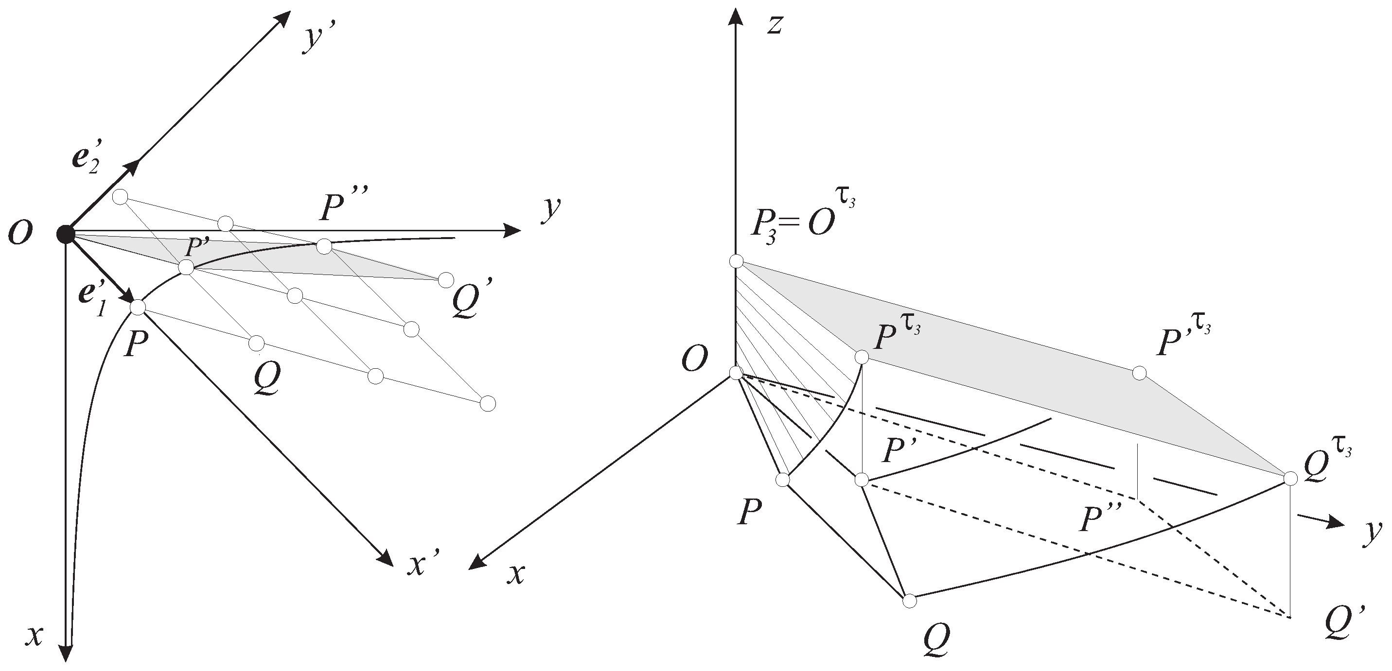
These (commutative group of) transforms commute with the matrix of Jordan form
1 1 0 0 0 1 1 0 0 0 1 0 0 0 0 1
( d s ) 2 = ( d x ) 2 + [ ( d x ) ( x ) + ( d y ) ] 2 + ( d z ) 2 = ( d x ) 2 ( 1 + x 2 ) 2 ( d x ) ( d y ) x + ( d y ) 2 + ( d z ) 2 ; leads to x = 0 , y x x = 0 , z = 0 , so with x ( 0 ) = u , y ( 0 ) = v , z ( 0 ) = w , u 2 + v 2 + w 2 = 1 , to x = u s , y = 1 2 u 2 s 2 + v s , z = w s ;
parabolas as geodesics for this geometry.
(ii)
These transforms commute with the matrix
1 1 0 0 0 1 1 0 0 0 1 1 0 0 0 1
( d s ) 2 = ( d x ) 2 + [ ( d x ) ( x ) + ( d y ) ] 2 + [ ( d x ) ( x 2 y ) + ( d y ) ( x ) + ( d z ) ] 2 = ( d x ) 2 ( 1 + x 2 + x 4 2 x 2 y + y 2 ) 2 ( d x ) ( d y ) ( x + x 3 x y ) + 2 ( d x ) ( d z ) ( x 2 y ) + ( d y ) 2 ( 1 + x ) 2 2 ( d y ) ( d z ) x + ( d z ) 2 ; leads to
x = 0 , y x x x = 0 , z + x x x 2 x y = 0 , so with x ( 0 ) = u , y ( 0 ) = v , z ( 0 ) = w , u 2 + v 2 + w 2 = 1 , to x = u s , y = 1 2 u 2 s 2 + v s , z = u 3 / 6 s 3 + u v s 2 + w s ;
we get cubics as geodesics for this geometry.
At the same time, in both cases (denote by ( T ) the given matrix), our geodesics are so-called translation curves, i.e., the solutions of the first order differential equation system (dynamical system with u 2 + v 2 + w 2 = 1 )
( 0 , u , v , w ) ( T ) = ( 0 , x , y , z ) .
Our “translations” in the above commutative Cases (i)–(ii) are seemingly diffeomorphically equivariant with some Euclidean translations. It would be nice to find a method (if there exists such) for recognizing well-known geometries to the above unknown matrices.
We have summarized in Table 1 the significant notions of the projective models of Thurston geometries:

2. Specific Geometries, H 2 × R and S L 2 R ˜ in Models

The Thurston geometries are well known. Here, E 3 , S 3 and H 3 are the classical spaces of constant zero, positive and negative sectional curvature, respectively; S 2 × R and H 2 × R are direct product geometries with S 2 spherical and H 2 hyperbolic base plane, respectively, and a distinguished R -line with usual R -metric; S L 2 R ˜ and Nil with a twisted product of R with H 2 and E 2 , respectively; and Sol as a twisted product of the Minkowski plane M 2 with R . Thus, we have, in each an infinitesimal (positive definite) Riemann metric, invariant under certain translations, guaranteing homogeneity in every point.
These translations commute only in E 3 , in general, but a discrete (discontinuous) translation group—as a lattice—can be defined with compact fundamental domain in Euclidean analogy, but with some different properties. The additional symmetries can define crystallographic groups with compact fundamental domain, again in Euclidean analogy, moreover with nice tilings, packings, material possibilities, etc.
Our projective spherical model, initiated in [1], is based on linear algebra over the real vector space V 4 (for points) and its dual V 4 (for planes) (see Figure 1), up to a positive real factor, so that the proper dimension is 3. We can illustrate and visualize the topic in the Euclidean screen of a computer.
Here, we mention only the model of the spaces H 2 × R and S L 2 R ˜ derived from the hyperbolic plane H 2 (see Figure 2 and Figure 3).

3. Crystallography in Non-Euclidean Spaces

3.1. Hyperbolic Space H 3

In n-dimensional hyperbolic space H n ( n 2 ) , there are 3-types of spheres (balls): the sphere, horosphere and hypersphere. If n = 2 , 3 we know a universal upper bound of the ball packing densities, where each ball volume is related to the volume of the corresponding Dirichlet–Voronoi (D-V) cell. For example, in H 3 , the densest horoball packing is derived from the { 3 , 3 , 6 } Coxeter tiling consisting of ideal regular simplices T r e g with dihedral angles π 3 . The density of this packing is δ 3 0.85328 and this provides a very rough upper bound for the ball packing densities as well. However, there are no “essential” results regarding the “classical” ball packings with congruent balls, nor for ball coverings.
In [8], we have studied the extremal ball arrangements in H 3 with “classical balls”. We consider only periodic congruent ball arrangements (for simplicity) related to the generalized, so-called complete Coxeter orthoschemes and their extended groups. We also formulated conjectures for the densest ball packing with density 0.77147 and the loosest ball covering with density 1.36893 . Both are related to the extended Coxeter group ( 5 , 3 , 5 ) and the so-called hyperbolic football manifold (look at Figure 4). These facts can have important relations with fullerenes in crystallography.
Imagine congruent football polyhedra filling hyperbolic space H 3 . The faces are paired (glued together), e.g., a 1 a will be mapped by a screw motion a , carrying F G into its adjacent F G a . Three footballs meet at each edge, and four meet at each vertex (as carbon atoms with 4 valences).
In [9], the second author classified the hyperbolic dodecahedron manifolds (see Figure 5).
As a byproduct of our papers [8,10], and the previous initiative of the first author, we have recently found an infinite sequence of hyperbolic polyhedra C w ( 2 z , 2 z , 2 z ) ( 6 2 z , 3 z odd integer) which can be equipped with a fixed-point-free face pairing, as a gluing procedure, so that the polyhedron become a compact hyperbolic manifold. That means each point has a ball-like neighbourhood. The visualization of such “finite worlds” seems to be a timely task, and we try to involve our students as well. First, we model the famous hyperbolic football manifold, and restrict ourselves only to the C w ( 6 , 6 , 6 ) manifold as in [11]. The description of fundamental groups and other properties, moreover visualization of such “finite worlds” seem to be interesting problems, as well (see Figure 6).
In the computations (e.g., [8,12]), we use the above orthoschemes whose volume is derived by the next theorem of R. Kellerhals ([13], using ingenious ideas of N. I. Lobachevsky):
Theorem 1.
(R. Kellerhals) The volume of a three-dimensional hyperbolic complete orthoscheme O = W u v w H 3 is expressed with the essential angles α 01 = π u , α 12 = π v , α 23 = π w , ( 0 α i j π 2 ) in the following form:
Vol ( O ) = 1 4 { L ( α 01 + θ ) L ( α 01 θ ) + L ( π 2 + α 12 θ ) + L ( π 2 α 12 θ ) + L ( α 23 + θ ) L ( α 23 θ ) + 2 L ( π 2 θ ) } ,
where θ [ 0 , π 2 ) is defined by:
tan ( θ ) = cos 2 α 12 sin 2 α 01 sin 2 α 23 cos α 01 cos α 23 ,
and where L ( x ) : = 0 x log | 2 sin t | d t denotes the Lobachevsky function (in J. Milnor’s interpretation).
The volume Vol ( B ( R ) ) of a ball B ( R ) of radius R can be computed by the classical formula of J. Bolyai:
Vol ( B ( R ) ) = 2 π ( cosh ( R ) sinh ( R ) R ) = π ( sinh ( 2 R ) 2 R ) = 4 3 π R 3 ( 1 + 1 5 R 2 + 2 105 R 4 + ) .

3.2. Nil Space

Nil-geometry is derived from the famous Heisenberg matrix group. It is one of the 8 Thurston 3-geometries, having also an affine-projective interpretation, as the first author initiated with his colleagues. The third author found a top dense lattice-like geodesic ball packing in Nil (of kissing number 14) (see [14]) with density 0.78085 denser than the best Euclidean one with π 3 2 0.74048 with kissing number 12 in the famous Kepler conjecture. If we linearize Nil , i.e., its translation curves, then the geodesic curve can explicitly be determined from the corresponding second order differential equation system. Geodesic spheres and balls can be attractively visualized using these results (see Figure 7).

3.3. Sol Space

In the eight homogeneous Thurston 3-geometries, the notions of translation curves and translation balls can be introduced in a unified way by the initiative of E. Molnár (see [15]). P. Scott in [16], who defined Sol lattices to which lattice-like translation ball packings can be investigated (see Figure 8 and Figure 9).
In [17] the third author has studied the relation between Sol lattices and lattices of the pseudoeuclidean (or Minkowskian) plane. We have investigated the translation balls of Sol space and computed their volume, defined the Sol parallelepiped and the density of the lattice-like ball packing. Moreover, the third author determined the densest translation ball packing by so-called fundamental lattices. This density is δ 0.56405 and the kissing number of the balls to this packing is 6. In our work, we used the affine model of Sol space through affine-projective homogeneous coordinates introduced by the first author in [1]. We only note here that the first and third authors in [7] classified the Sol lattices (see [18]).

3.4. S 2 × R Space

In [19], the third author described a candidate of the densest geodesic ball packing for all Thurston geometries. The greatest density until now was ≈ 0.85328 that is not realized by a packing with equal balls of H 3 . However, that is attained, in different manners, e.g., by a horoball packing of hyperbolic space H ¯ 3 where the ideal centres of horoballs lie on the absolute figure of H ¯ 3 inducing the regular ideal simplex tiling ( 3 , 3 , 6 ) by its Coxeter–Schläfli symbol. In [19], the third author presented a geodesic ball packing whose density is ≈ 0.87757 in S 2 × R geometry. The extremal configuration is illustrated in Figure 10. Moreover, in [19], it has been formulated, as a conjectute, that is the densest geodesic ball packing with equal balls for all Thurston geometries.

4. Conclusions

In this paper (related to the 10th BGL 2017 Gyöngyös/Hungary), based on the presentation of the first author, we have motivated our new initiative on projective interpretation of the 8 Thurston geometries, where open problems arise as well. After illustrating some specific geometries, we have presented new hyperbolic space forms with possible applications in crystallography. Thus, the hyperbolic football manifolds [20] as fullerenes, then brand new infinite series of cobweb (tube) manifolds as nanotubes have been introduced [11]. Various ball packing and covering problems have been reported as new mathematical results, as well as with possible applications.
We kindly refer the interested reader to the further works [19,21,22,23,24,25,26,27]. The authors thank the referees for their kind help in improving the style of this paper.

Conflicts of Interest

The authors declare no conflict of interest.

References

  1. Molnár, E. The projective interpretation of the eight 3-dimensional homogeneous geometries. Beitr. Algebra Geom. Contrib. Algebra Geom. 1997, 38, 261–288. [Google Scholar]
  2. Molnár, E.; Szirmai, J. Symmetries in the 8 homogeneous 3-geometries. Symmetry Cult. Sci. 2010, 21, 87–117. [Google Scholar]
  3. Molnár, E.; Prok, I.; Szirmai, J. The Euclidean visualization and projective modelling the 8 Thurston geometries. Stud. Univ. Zilina Math. Ser. 2015, 27, 35–62. [Google Scholar]
  4. Molnár, E.; Prok, I.; Szirmai, J. Classification of tile-transitive 3-simplex tilings and their realizations in homogeneous spaces. In Non-Euclidean Geometries, János Bolyai Memorial Volume, Mathematics and Its Applications; Prékopa, A., Molnár, E., Eds.; Springer: Boston, MA, USA, 2006; Volume 581, pp. 321–363. [Google Scholar]
  5. Molnár, E.; Szirmai, J.; Vesnin, A. Packings by translation balls in S L 2 R ˜ . J. Geom. 2014, 105, 287–306. [Google Scholar] [CrossRef]
  6. Molnár, E.; Szirmai, J.; Vesnin, A. Geodesic and translation ball packings generated by prismatic tessellations of the universal cover of SL2R. Results Math. 2017, 71, 623–642. [Google Scholar] [CrossRef]
  7. Molnár, E.; Szirmai, J. Classification of Sol lattices. Geom. Dedicata 2012, 161, 251–275. [Google Scholar] [CrossRef]
  8. Molnár, E.; Szirmai, J. Top dense hyperbolic ball packings and coverings for complete Coxeter orthoscheme groups. arXiv, 2017; arXiv:161204541v1. [Google Scholar]
  9. Prok, I. Classification of dodecahedral space forms. Beitr. Algebra Geom. Contrib. Algebra Geom. 1998, 39, 497–515. [Google Scholar]
  10. Molnár, E. Polyhedron complexes with simply transitive group actions and their realizations. Acta Math. Hung. 1991, 59, 175–216. [Google Scholar]
  11. Molnár, E.; Szirmai, J. On hyperbolic cobweb manifolds. Stud. Univ. Zilina Math. Ser. 2016, 28, 43–52. [Google Scholar]
  12. Szirmai, J. The optimal ball and horoball packings to the Coxeter honeycombs in the hyperbolic d-space. Beitr. Algebra Geom. Contrib. Algebra Geom. 2007, 48, 35–47. [Google Scholar]
  13. Kellerhals, R. On the volume of hyperbolic polyhedra. Math. Ann. 1989, 245, 541–569. [Google Scholar] [CrossRef]
  14. Szirmai, J. The densest geodesic ball packing by a type of Nil lattices. Beitr. Algebra Geom. 2007, 48, 383–397. [Google Scholar]
  15. Molnár, E.; Szilágyi, B. Translation curves and their spheres in homogeneous geometries. Publ. Math. Debr. 2011, 78, 327–346. [Google Scholar] [CrossRef]
  16. Scott, P. The geometries of 3-manifolds. Bull. Lond. Math. Soc. 1983, 15, 401–487. [Google Scholar] [CrossRef]
  17. Szirmai, J. The densest translation ball packing by fundamental lattices in Sol space. Beitr. Algebra Geom. Contrib. Algebra Geom. 2010, 51, 353–373. [Google Scholar]
  18. Cavichioli, A.; Molnár, E.; Spaggiari, F.; Szirmai, J. Some tetrahedron manifolds with Sol geometry. J. Geom. 2014, 105, 601–614. [Google Scholar] [CrossRef]
  19. Szirmai, J. A candidate to the densest packing with equal balls in the Thurston geometries. Beitr. Algebra Geom. 2014, 55, 441–452. [Google Scholar] [CrossRef]
  20. Molnár, E. Two hyperbolic football manifolds. In Proceedings of the International Conference on Differential Geometry and Its Applications, Dubrovnik, Yugoslavia, 26 June 1988; pp. 217–241. [Google Scholar]
  21. Molnár, E. Projective Metrics and hyperbolic volume. Ann. Univ. Sci. Budap., Sect. Math. 1989, 32, 127–157. [Google Scholar]
  22. Molnár, E. Combinatorial construction of tilings by barycentric simplex orbits (D symbols) and their realizations in Euclidean and other homogeneous spaces. Acta Cryst. 2005, A61, 542–552. [Google Scholar] [CrossRef] [PubMed]
  23. Prok, I. Data structures and procedures for a polyhedron algorithm. Period. Polytech. Ser. Mech. Eng. 1992, 36, 299–316. [Google Scholar]
  24. Szirmai, J. Geodesic ball packing in S2 × R space for generalized Coxeter space groups. Beitr. Algebra Geom. Contrib. Algebra Geom. 2011, 52, 413–430. [Google Scholar] [CrossRef]
  25. Szirmai, J. Lattice-like translation ball packings in Nil space. Publ. Math. Debr. 2012, 80, 427–440. [Google Scholar] [CrossRef]
  26. Weeks, J.R. Real-time animation in hyperbolic, spherical, and product geometries. In Non-Euclidean Geometries, János Bolyai Memorial Volume, Mathematics and Its Applications; Prékopa, A., Molnár, E., Eds.; Springer: Boston, MA, USA, 2006; Volume 581, pp. 287–305. [Google Scholar]
  27. Wildberger, N.J. Universal hyperbolic geometry, sydpoints and finite fields: A projective and algebraic alternative. Universe 2017. submitted. [Google Scholar]
Figure 1. Our scene for dimensions 2 with projective sphere P S 2 embedded into the real vector space V 3 and its dual V 3 .
Universe 03 00083 g001
Figure 2. The hyperbolic plane H 2 , embedded into P 2 P S 2 by a conic polarity u ( u ) U ( u ) , p P , a A (the Beltrami–Cayley–Klein disc model). Here, we illustrate the projective model of H 2 × R geometry, too. Imagine similarities from the origin O. The logarithm of similarity factor will be the R -parameter.
Universe 03 00083 g002
Figure 3. The unparted hyperboloid model of S L 2 R ˜ = H ˜ of skew line fibres growing in points of a hyperbolic base plane H 2 . In addition, a Gum-fibre model of Hans Havlicek and Rolf Riesinger, used also by Hellmuth Stachel with other respects (Vienna UT).
Universe 03 00083 g003
Figure 4. The hyperbolic football manifold for the Archimedean solid { 5 , 6 , 6 } and fullerenes.
Universe 03 00083 g004
Figure 5. Twofold covering the football manifold as a hyperbolic dodecahedron manifold.
Universe 03 00083 g005
Figure 6. Cobweb manifold C w ( 6 , 6 , 6 ) as a nanotube.
Universe 03 00083 g006
Figure 7. The densest lattice-like congruent ball configuration in Nil space related to the lattice parameter k = 1 , the central red ball is touching 14 surrounding green ones (computer picture by Benedek Schultz), and a horizontal geodesic curve lying in a hyperbolic paraboloid.
Universe 03 00083 g007
Figure 8. Fundamental lattice in Sol geometry. Notice the Minkowskian base lattice of special relativity.
Universe 03 00083 g008
Figure 9. The optimal translation ball arrangement by fundamental lattices in Sol space.
Universe 03 00083 g009
Figure 10. The conjectured densest geodesic ball packing configuration for all Thurston geometries in the specific projective model of S 2 × R geometry whose density is ≈0.87757⋯
Universe 03 00083 g010
Table 1. Thurston geometries each modelled on P S 3 by specified polarity or scalar product and isometry group.
Space XSignature of Polarity Π ( ) or Scalar Product , in V 4 Domain of Proper Points of X in P S 3 ( V 4 ( R ) , V 4 ) The Group G = Isom X as a Special Collineation Group of P S 3
S 3 ( + + + + ) P S 3 Coll P S 3 preserving Π ( )
H 3 ( + + + ) { ( x ) P 3 : x , x < 0 } Coll P 3 preserving Π ( )
S L 2 R ˜ ( + + ) with skew line fiberingUniversal covering of H : = { [ x ] P S 3 : x , x < 0 } by fibering transformationsColl P 3 preserving Π ( ) generated by plane reflections
E 3 ( 0 + + + ) A 3 = P 3 \ { ω } where ω : = ( b 0 ) , b 0 = 0 Coll P 3 preserving Π ( ) , generated by plane reflections
S 2 × R ( 0 + + + ) with O-line bundle fibering A 3 \ { O } , O is a fixed originG is generated by plane reflections and sphere inversions, leaving invariant the O-concentric 2-spheres of  Π ( )
H 2 × R ( 0 + + ) with O-line bundle fibering C + = { X A 3 : O X , O X < 0 , half cone} by fiberingG is generated by plane reflections and hyperboloid inversions, leaving invariant the O-concentric half-hyperboloids in the half-cone  C + by Π ( )
Sol ( 0 + + ) and parallel plane fibering with an ideal plane ϕ A 3 = P 3 \ ϕ Coll. of A 3 preserving Π ( ) and the fibering with 3 parameters
Nil Null-polarity Π ( ) with parallel line bundle fibering F with its polar ideal plane ϕ A 3 = P 3 \ ϕ Coll. of A 3 preserving Π ( ) with 4 parameters

