Perturbative Accelerating Solutions of Relativistic Hydrodynamics

Abstract

In ultra-relativistic collisions of heavy ions, the strongly interacting Quark Gluon Plasma (sQGP) is created. The fluid nature of the sQGP was one of the important discoveries of high energy heavy ion physics in the last decades. Henceforth the explosion of this matter may be described by hydrodynamical models. Besides numerical simulations, it is important to study the analytic solutions of the equations of hydrodynamics, as these enable us to understand the connection of the final and initial states better. In this paper we present a perturbative, accelerating solution of relativistic hydrodynamics, on top of a known class of solutions describing Hubble-expansion. We describe the properties of this class of perturbative solutions, and investigate a few selected solutions in detail.

1. Introduction

The equations of perfect hydrodynamics have no internal scale, and hence they describe aspects of the time evolution of systems with vastly different sizes: from galactic clusters and galaxies through stars, planets and human-scale systems, down to the femtometer scale sQGP, created in heavy ion collisions at RHIC [1,2] and the LHC [3,4,5,6]. The sQGP is formed in heavy ion collisions after an initial thermalization time $\mathcal{O}(1\mathrm{fm}/c)$, its evolutions lasts $\mathcal{O}(10\mathrm{fm}/c)$, after that it creates hadrons in the hadronization. We observe these hadrons, and hydrodynamics may be used to infer the time evolution and the initial state from the hadron final state distributions.

Hydrodynamics is based on the local conservation of energy and momentum, expressed through

$$\begin{array}{c}\hfill {\partial }_{\nu }{T}^{\mu \nu }=0,\end{array}$$

(1)

with $T^{\mu \nu }$ being the energy-momentum tensor. In case of a perfect fluid, this can be written as

$$\begin{array}{c}\hfill T^{\mu \nu }=(ϵ+p)u^{\mu }{u}^{\nu }-p{g}^{\mu \nu }.\end{array}$$

(2)

where $u^{\mu }$ is the flow field (subject to the $u_{\mu }{u}^{\mu }=1$ constraint), $ϵ$ is the energy density, p is the pressure and $g^{\mu \nu }$ is the metric tensor, $\mathrm{diag}(1,-1,-1,-1)$. The Equation of State (EoS) closes this set of equations:

$$\begin{array}{c}\hfill ϵ=\kappa p\end{array}$$

(3)

where $\kappa$ is the EoS parameter, which may depend on the temperature. In this paper we assume constant values, even if $\kappa (T)$ type of solutions of relativistic hydrodynamics are know [7]. In case of the above described perfect fluid, continuity for the entropy density $\sigma =(ϵ+p)/T$ follows from the above equations, and a similar continuity equation for the density of some conserved charge (n) may be prescribed:

$$\begin{array}{c}\hfill {\partial }_{\mu }(\sigma u^{\mu })=0,\end{array}$$

(4)

$$\begin{array}{c}\hfill {\partial }_{\mu }(n{u}^{\mu })=0.\end{array}$$

(5)

With this, a solution of the equations is a set of fields $(u^{\mu },p,n)$ or $(u^{\mu },p,\sigma )$, given in terms of coordinates $x^{\mu }$, where sometimes also the coordinate proper-time is introduced as $\tau =\sqrt{x_{\mu }{x}^{\mu }}$, along some scaling variable $s(x^{\mu })$ that describes the spatial profile of the densities in the solution.

The discovery of the fluid nature of the sQGP produced a revival of interest for solutions of hydrodynamics, beyond the well-known Landau-Khalatnikov [8,9] and Hwa-Bjorken [10,11] solutions. Besides numerical simulations (see e.g. Refs. [12,13,14] for recent examples), multiple advanced analytic solutions were found in the last decade [7,15,16,17,18,19,20,21]. One important example is the simple, ellipsoidal Hubble-flow described in Ref. [15], which describes hadron and photon observables well [22,23]. However, this solution lacks acceleration, and while Hubble-flow is natural in the final state, initial pressure gradients may be important in understanding the time evolution of this system. In this paper we attempt to find accelerating perturbations on top of Hubble-flow.

2. Perturbative Solutions of Hydrodynamics

The equation for the conservation of energy and momentum density, Equation (1) may be projected onto $u^{\mu }$, producing a Lorentz-parallel and a Lorentz-orthogonal equation, similarly to Refs. [7,17]:

$$\begin{array}{c}\hfill \kappa u^{\mu }{\partial }_{\mu }p+(\kappa +1)p{\partial }_{\mu }{u}^{\mu }=0\end{array}$$

(6)

$$\begin{array}{c}\hfill (\kappa +1)p{u}^{\mu }{\partial }_{\mu }{u}^{\nu }=(g^{\mu \nu }-u^{\mu }{u}^{\nu }){\partial }_{\mu }p,\end{array}$$

(7)

where the first is called the energy equation, and the second is the Euler equation of relativistic hydrodynamics. If a given solution is given in terms of $(u^{\mu },p,n)$, then perturbations on top of this solution may be given as:

$$\begin{array}{cc}\hfill u^{\mu }& \to u^{\mu }+\delta u^{\mu },\hfill \end{array}$$

(8)

$$\begin{array}{cc}\hfill p& \to p+\delta p,\hfill \end{array}$$

(9)

$$\begin{array}{cc}\hfill n& \to n+\delta n,\hfill \end{array}$$

(10)

where we restrict ourselves to a conserved charge here, but the continuity may be understood for the entropy density just as well. Now if these perturbations are small, then the equations of hydrodynamics may be given in first order. First of all, the perturbations of the flow field must fulfill

$$\begin{array}{c}\hfill (u^{\mu }+\delta u^{\mu })(u_{\mu }+\delta u_{\mu })=1\end{array}$$

(11)

which yields the first order equation of

$$\begin{array}{c}\hfill u_{\mu }\delta u^{\mu }=0.\end{array}$$

(12)

With this, we may substitute the perturbed fields in Equations (8)–(10) into the equations of hydrodynamics, Equations (5)–(7). For the continuity equation, we get the following first order equation:

$$\begin{array}{c}\hfill u^{\mu }{\partial }_{\mu }\delta n+\delta n{\partial }_{\mu }{u}^{\mu }+\delta u^{\mu }{\partial }_{\mu }n+n{\partial }_{\mu }\delta u^{\mu }=0.\end{array}$$

(13)

For the energy equation, we obtain:

$$\begin{array}{c}\hfill \kappa \delta u^{\mu }{\partial }_{\mu }p+\kappa u^{\mu }{\partial }_{\mu }\delta p+(\kappa +1)\delta p{\partial }_{\mu }{u}^{\mu }+(\kappa +1)p{\partial }_{\mu }\delta u^{\mu }=0.\end{array}$$

(14)

And for the Euler-equation, the first order perturbative equation is

$$(\kappa +1)\delta p{u}^{\mu }{\partial }_{\mu }{u}^{\nu }+(\kappa +1)p\delta u^{\mu }{\partial }_{\mu }{u}^{\nu }+(\kappa +1)p{u}^{\mu }{\partial }_{\mu }\delta u^{\nu }=(g^{\mu \nu }-u^{\mu }{u}^{\nu }){\partial }_{\mu }\delta p-\delta u^{\mu }{u}^{\nu }{\partial }_{\mu }p-u^{\mu }\delta u^{\nu }{\partial }_{\mu }p.$$

(15)

To perform a basic consistency check of the above equations, one may investigate what happens when the basic solution of a fluid at rest. The flow and pressure is then

$$\begin{array}{c}\hfill u_{\mu }=(1,0,0,0) \mathrm{and} p=p_0.\end{array}$$

(16)

One may immediately observe, that ${\partial }_{\mu }{u}^{\mu }=0$, ${\partial }_{\mu }p=0$, and $u^{\mu }{\partial }_{\mu }={\partial }_t$. With this, the linearized energy and Euler equations become

$$\begin{array}{cc}\hfill \kappa {\partial }_t\delta p+(\kappa +1)p{\partial }_{\mu }\delta u^{\mu }& =0,\hfill \end{array}$$

(17)

$$\begin{array}{cc}\hfill (\kappa +1)p{\partial }_t\delta u^{\nu }-(u^{\mu }{u}^{\nu }-g^{\mu \nu }){\partial }_{\mu }\delta p& =0.\hfill \end{array}$$

(18)

The time derivative of the energy equation is then

$$\begin{array}{c}\hfill \kappa {\partial }_t^2\delta p+(\kappa +1)p{\partial }_t{\partial }_{\mu }\delta u^{\mu }=0.\end{array}$$

(19)

Let us then introduce the $Q^{\mu \nu }=(u^{\mu }{u}^{\nu }-g^{\mu \nu })$ operator — which is here nothing else than $\mathrm{diag}(0,1,1,1)$. Then the effect of $Q_{\rho \nu }{\partial }^{\rho }$ on the Euler equation is

$$\begin{array}{c}\hfill (\kappa +1)p{\partial }_t{\partial }_{\nu }\delta u^{\nu }+\Delta \delta p=0,\end{array}$$

(20)

where we observed that

$$\begin{array}{c}\hfill Q_{\rho \nu }{\partial }^{\rho }{Q}^{\mu \nu }{\partial }^{\mu }=({\partial }_x^2+{\partial }_y^2+{\partial }_z^2)=\Delta .\end{array}$$

(21)

From Equations (19) and (20), we obtain

$$\begin{array}{c}\hfill {\partial }_t^2\delta p-\frac{1}{\kappa }\Delta \delta p=0,\end{array}$$

(22)

which means that, as expected, pressure perturbations behave as waves with a speed of sound of $c_s=1/\sqrt{\kappa }$.

3. Perturbations on Top of Hubble-Flow

As mentioned above, in Ref. [15] a Hubble-type of self-similar solution is given, with a flow field

$$\begin{array}{c}\hfill u^{\mu }=\frac{x^{\mu }}{\tau },\end{array}$$

(23)

where again ${\tau }^2=x^{\mu }{x}_{\mu }$ is the coordinate proper-time. The basic quantity of this solution is the scale variable assuring self-similarity, for which the comoving derivative vanishes:

$$\begin{array}{c}\hfill u^{\mu }{\partial }_{\mu }S=0.\end{array}$$

(24)

Since in this case, $u^{\mu }{\partial }_{\mu }={\partial }_{\tau }$, the following simple pressure field and density can be obtained:

$$\begin{array}{cc}\hfill n& =n_0{\left(\frac{{\tau }_0}{\tau }\right)}^3\mathcal{N}(S),\hfill \end{array}$$

(25)

$$\begin{array}{cc}\hfill p& =p_0{\left(\frac{{\tau }_0}{\tau }\right)}^{3+\frac{3}{\kappa }},\hfill \end{array}$$

(26)

where $\mathcal{N}(S)$ is an arbitrary scale function. This solution can be generalized to describe multipole type of scale variables [21], but a standard choice yielding ellipsoidal symmetry is

$$\begin{array}{c}\hfill S=\frac{x^2}{X^2}+\frac{y^2}{Y^2}+\frac{z^2}{Z^2}\end{array}$$

(27)

with the coordinates given as $x,y,z$, and the axes of the expanding ellipsoid are $X,Y,Z$, all linear in time. We will focus here on the spherical case:

$$\begin{array}{c}\hfill S=\frac{r^2}{{\dot{R}}_0^2{t}^2},\end{array}$$

(28)

where r is the radial coordinate, and ${\dot{R}}_0$ describes the expansion velocity of the scale of the solution. This solution yields the following equations for the perturbations of the fields:

$$\begin{array}{cc}\hfill \delta u^{\mu }n\frac{{\mathcal{N}}^{\prime }}{\mathcal{N}}{\partial }_{\mu }S+u^{\mu }{\partial }_{\mu }\delta n+\frac{3\delta n}{\tau }+n{\partial }_{\mu }\delta u^{\mu }& =0,\hfill \end{array}$$

(29)

$$\begin{array}{cc}\hfill \kappa u^{\mu }{\partial }_{\mu }\delta p+\frac{3(\kappa +1)}{\tau }\delta p& =-(\kappa +1)p{\partial }_{\mu }\delta u^{\mu },\hfill \end{array}$$

(30)

$$\begin{array}{cc}\hfill \frac{{\partial }_{\mu }\delta p}{(\kappa +1)p}\left[g^{\mu \nu }-u^{\mu }{u}^{\nu }\right]& =\frac{\kappa -3}{\tau \kappa }\delta u^{\nu }+u^{\mu }{\partial }_{\mu }\delta u^{\nu }.\hfill \end{array}$$

(31)

A similar setup was investigated in Ref. [24], where the authors found expressions for the ripples propagating on Hubble-flow. Unlike Ref. [24], we will now discuss global perturbations in terms of $\delta u^{\mu }$, $\delta p$ and $\delta n$.

In this proceedings paper we do not detail the way this solution was obtained, but simply present the result for the flow, pressure and density:

$$\begin{array}{cc}\hfill \delta u^{\mu }& =\delta ·F(\tau )g(x^{\mu })\chi (S){\partial }^{\mu }S,\hfill \end{array}$$

(32)

$$\begin{array}{cc}\hfill \delta p& =\delta ·p_0{\left(\frac{{\tau }_0}{\tau }\right)}^{3+\frac{3}{\kappa }}\pi (S),\hfill \end{array}$$

(33)

$$\begin{array}{cc}\hfill \delta n& =\delta ·n_0{\left(\frac{{\tau }_0}{\tau }\right)}^{3}h(x^{\mu })\nu (S),\hfill \end{array}$$

(34)

where S is the scale variable (with vanishing comoving derivative), $\delta$ is the perturbation scale, c is an arbitrary constant, $F,h,g$ are profile functions, while $\pi$, $\chi$, $\nu$ are scale functions subject to the following condition equations:

$$\begin{array}{cc}\hfill \frac{{\chi }^{\prime }(S)}{\chi (S)}& =-\frac{{\partial }_{\mu }{\partial }^{\mu }S}{{\partial }_{\mu }S{\partial }^{\mu }S}-\frac{{\partial }_{\mu }S{\partial }^{\mu }lng(x^{\mu })}{{\partial }_{\mu }S{\partial }^{\mu }S},\hfill \end{array}$$

(35)

$$\begin{array}{cc}\hfill \frac{{\pi }^{\prime }(S)}{\chi (S)}& =(\kappa +1)\left[F(\tau )\left(u^{\mu }{\partial }_{\mu }g(x^{\mu })-\frac{3g(x^{\mu })}{\kappa \tau }\right)+F^{\prime }(\tau )g(x^{\mu })\right],\hfill \end{array}$$

(36)

$$\begin{array}{cc}\hfill \frac{\nu (S)}{\chi (S){\mathcal{N}}^{\prime }(S)}& =-\frac{F(\tau )g(x^{\mu }){\partial }_{\mu }S{\partial }^{\mu }S}{u^{\mu }{\partial }_{\mu }h(x^{\mu })}.\hfill \end{array}$$

(37)

In simple terms, these equations can be translated to the following conditions:

• The scale variable S fulfills $u_{\mu }{\partial }^{\mu }S=0$ with the original flow field.
• The right hand sides of Equations (35)–(37) depends only on S.

First of all, let us restrict ourselves to the simplest case of $g(x^{\mu })=1$ here, in order to describe the way this class of perturbative solutions works. This gives a simple form for F as

$$\begin{array}{c}\hfill F(\tau )=\tau +c{\tau }_0{\left(\frac{\tau }{{\tau }_0}\right)}^{\frac{3}{\kappa }}.\end{array}$$

(38)

Then let us select an h function that leads to simpler condition equations:

$$\begin{array}{cc}\hfill h(x^{\mu })& =ln\left(\frac{\tau }{{\tau }_0}\right)+\frac{c\kappa }{3-\kappa }{\left(\frac{\tau }{{\tau }_0}\right)}^{\frac{3}{\kappa }-1},( \mathrm{if} \kappa \ne 3),\hfill \end{array}$$

(39)

$$\begin{array}{cc}\hfill h(x^{\mu })& =(1+c)ln\left(\frac{\tau }{{\tau }_0}\right),( \mathrm{if} \kappa =3).\hfill \end{array}$$

(40)

The above choices of transforms Equations (35)–(37) to the simple equations of

$$\begin{array}{cc}\hfill \frac{{\chi }^{\prime }(S)}{\chi (S)}& =-\frac{{\partial }_{\mu }{\partial }^{\mu }S}{{\partial }_{\mu }S{\partial }^{\mu }S},\hfill \end{array}$$

(41)

$$\begin{array}{cc}\hfill \frac{{\pi }^{\prime }(S)}{\chi (S)}& =\frac{(\kappa +1)(\kappa -3)}{\kappa }\hfill \end{array}$$

(42)

$$\begin{array}{cc}\hfill \frac{\nu (S)}{\chi (S){\mathcal{N}}^{\prime }(S)}& =-{\tau }^2{\partial }_{\mu }S{\partial }^{\mu }S.\hfill \end{array}$$

(43)

While more general solutions can also be found, a broad class of perturbative solutions can already be given, if suitable S scale variables and associated $\pi$, $\chi$, $\nu$ and h functions are found. Such suitable scale variables include

$$\begin{array}{c}\hfill S=\frac{r^m}{t^m},S=\frac{r^m}{{\tau }^m},S=\frac{{\tau }^m}{t^m}.\end{array}$$

(44)

In the next section, we will detail one particular sub-class of this class of solutions.

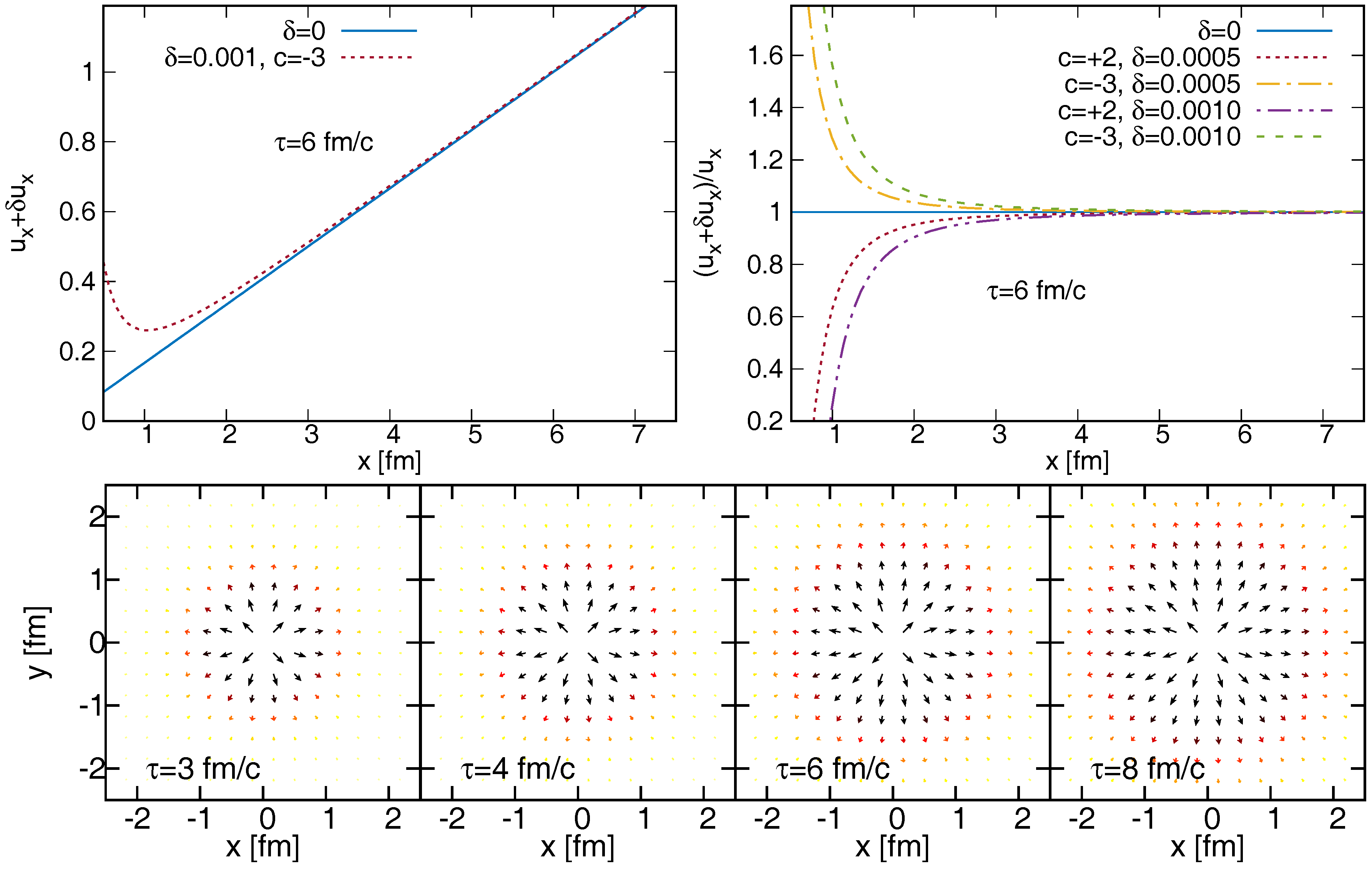
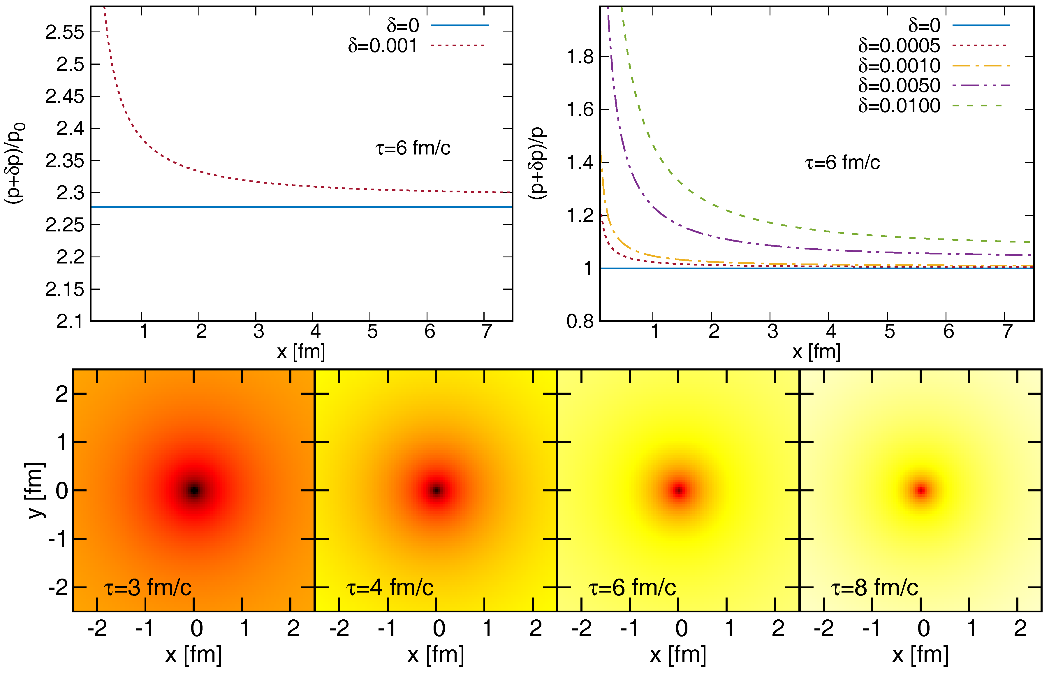
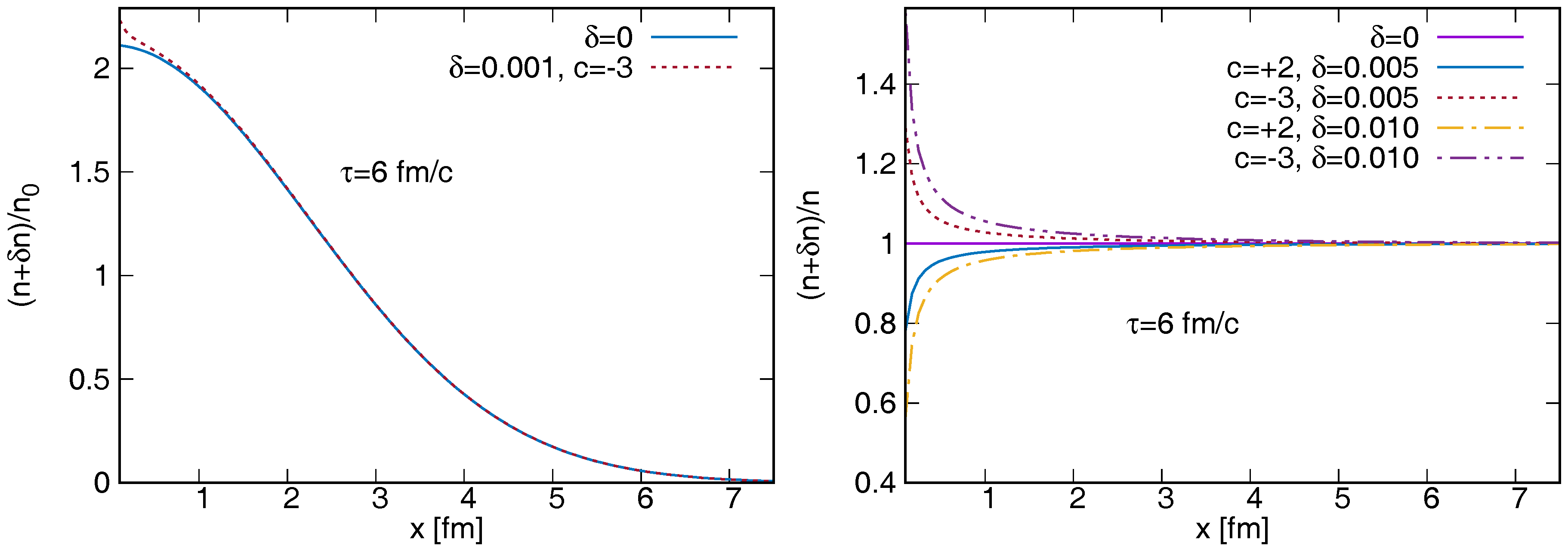
4. A Selected Sub-Class of Perturbative Solutions

If we introduce h as given in Equations (39)–(40) and S as $r^m/t^m$, we obtain the following scale functions:

$$\begin{array}{cc}\hfill \chi (S)& =S^{-\frac{m+1}{m}},\hfill \end{array}$$

(45)

$$\begin{array}{cc}\hfill \pi (S)& =-\frac{(\kappa +1)(\kappa -3)}{\kappa }m{S}^{-\frac{1}{m}},\hfill \end{array}$$

(46)

$$\begin{array}{cc}\hfill \nu (S)& =m^2{S}^{\frac{m-1}{m}}\left(S^{\frac{2}{m}}-1\right)\left(1-S^{-\frac{2}{m}}\right){\mathcal{N}}^{\prime }(S).\hfill \end{array}$$

(47)

This sub-class of solutions contains an arbitrary parameter c, the $\delta$ perturbation scale, the m exponent and the $\mathcal{N}(S)$ scale function (included in the original Hubble-solution as well). Let us chose $m=-1$, then the scale functions are

$$\begin{array}{cc}\hfill \chi (S)& =1,\hfill \end{array}$$

(48)

$$\begin{array}{cc}\hfill \pi (S)& =\frac{(\kappa +1)(\kappa -3)}{\kappa }S,\hfill \end{array}$$

(49)

$$\begin{array}{cc}\hfill \nu (S)& ={\left(1-S^2\right)}^2{\mathcal{N}}^{\prime }(S).\hfill \end{array}$$

(50)

Let us furthermore choose a suitable $\mathcal{N}$, leading to a Gaussian profile:

$$\begin{array}{c}\hfill \mathcal{N}(S)=e^{-b{S}^{-2}}=e^{-b\frac{r^2}{t^2}}\end{array}$$

(51)

With these, the perturbed fields (for $\kappa \ne 3$, the special case of $\kappa =3$ is discussed in Equation (40)) are as follows:

$$\begin{array}{cc}\hfill \delta u^{\mu }& =\delta ·\left[\tau +c{\tau }_0{\left(\frac{\tau }{{\tau }_0}\right)}^{\frac{3}{\kappa }}\right]{\partial }^{\mu }S,\hfill \end{array}$$

(52)

$$\begin{array}{cc}\hfill \delta p& =\delta ·p_0{\left(\frac{{\tau }_0}{\tau }\right)}^{3+\frac{3}{\kappa }}\frac{(\kappa +1)(\kappa -3)}{\kappa }S,\hfill \end{array}$$

(53)

$$\begin{array}{cc}\hfill \delta n& =\delta ·n_0{\left(\frac{{\tau }_0}{\tau }\right)}^3\left[ln\left(\frac{\tau }{{\tau }_0}\right)+c\frac{\kappa }{3-\kappa }{\left(\frac{\tau }{{\tau }_0}\right)}^{\frac{3}{\kappa }-1}\right]S^{-3}{\left(1-S^2\right)}^{2}2b\mathcal{N}(S).\hfill \end{array}$$

(54)

For the visualisation of these fields, let us chose parameter values from Refs. [22,23] as ${\tau }_0=7.7\mathrm{fm}/c$, $\kappa =10$ and $b=-0.1$.

On the top left panel of Figure 1, a slice of the x component of the flow field is shown with $\tau =6$ fm/c, $c=-3$ and $\delta =0.001$. The perturbation is the most important in the center, it also changes the direction of the field, but it vanishes for large radial distances. The top right panel indicates the c and $\delta$ dependence of the relative perturbed fields. We observe here that for this particular solution, the relative perturbation increases to very large values for very small distances. The bottom panel of Figure 1 indicates the transverse flow field for various proper-time slices, showing that also the direction of the flow is perturbed for some particular distances. Next, let us investigate the pressure perturbation. The top panels of Figure 2 shows the pressure field with fixed values of $\delta =0.001$ and $\tau =6$ fm/c (there is no c-dependence in p). Again it is clear that the perturbation vanishes for increasing radial distance, and increases for small distances. It is an important next step to present a sub-class of perturbative solutions that does not exhibit this feature. One may also note that $\delta$ controls the perturbation magnitude, as also visible in the ratio plots in the top right panel of Figure 2. On the bottom panel, the time evolution of the pressure perturbation is given in the transverse plane, showing a vanishing perturbation for large times. Finally, let us investigate the behavior of the density n. The left panel of Figure 3 (with $\tau =6$ fm/c, $\delta =0.001$ and $c=-3$) indicates again a vanishing perturbation for large distances. The right panel shows the relative perturbation and its dependence on $\delta$ and c. As it can be seen also in the figures, the perturbations become larger than the original fields for very small radial distances and large $\delta$ values, i.e. the method breaks down in these cases. This sets a limit to the applicability of the particular investigated perturbative solutions. Note however, that this is not necessarily a general property of the whole class of solutions.

With these fields at hand, and utilizing a freeze-out hypersurface similarly to e.g., Ref. [22], one may evaluate observables such as transverse momentum distribution, flow and Bose-Einstein correlation radii. We plan to do this in a subsequent publication.

5. Conclusions

In this paper we presented the method of obtaining perturbative solutions of relativistic hydrodynamics on top of known solutions. A new perturbative class of solutions on top of Hubble flow was discussed, and the modified fields were investigated in detail. These fields were scaled to a single $\delta$ perturbation parameter, and several scale functions appeared, subject to condition equations. As a subsequent step, we plan to describe more particular sub-classes of solutions. We also plan to calculate the modification of observables and in case of realistic geometries, we plan to compare them to measurements.

References

1. Adcox, K.; Adler, S.S.; Afanasiev, S.; Aidala, C.; Ajitanand, N.N.; Akiba, Y.; Al-Jamel, A.; Alexander, J.; Amirikas, R.; Aoki, K.; et al. Formation of dense partonic matter in relativistic nucleus nucleus collisions at RHIC: Experimental evaluation by the PHENIX collaboration. Nucl. Phys. 2005, 757, 184–283. [Google Scholar] [CrossRef]
2. Adams, J.; Aggarwal, M.M.; Ahammed, Z.; Amonett, J.; Anderson, B.D.; Arkhipkin, D.; Averichev, G.S.; Badyal, S.K.; Bai, Y.; Balewski, J.; et al. Experimental and theoretical challenges in the search for the quark gluon plasma: The STAR collaboration’s critical assessment of the evidence from RHIC collisions. Nucl. Phys. 2005, 757, 102–183. [Google Scholar] [CrossRef]
3. Aamodt, K.; Abrahantes Quintana, A.; Adamová, D.; Adare, A.M.; Aggarwal, M.M.; Aglieri Rinella, G.; Agocs, A.G.; Aguilar Salazar, S.; Ahammed, Z.; Ahmad, N.; et al. Suppression of Charged Particle Production at Large Transverse Momentum in Central Pb–Pb Collisions at s N N = 2.76 TeV. Phys. Lett. 2011, 696, 30–39. [Google Scholar] [CrossRef]
4. Aamodt, K.; Abelev, B.; Abrahantes Quintana, A.; Adamová, D.; Adare, A.M.; Aggarwal, M.M.; Aglieri Rinella, G.; Agocs, A.G.; Aguilar Salazar, S.; Ahammed, Z.; et al. Elliptic flow of charged particles in Pb-Pb collisions at 2.76 TeV. Phys. Rev. Lett. 2010, 105, 252302. [Google Scholar] [CrossRef] [PubMed]
5. Chatrchyan, S.; Khachatryan, V.; Sirunyan, A.M.; Tumasyan, A.; Adam, W.; Bergauer, T.; Dragicevic, M.; Erö, J.; Fabjan, C.; Friedl, M.; et al. Study of high-pT charged particle suppression in PbPb compared to pp collisions at s N N = 2.76 TeV. Eur. Phys. J. C 2012, 72, 1945. [Google Scholar] [CrossRef]
6. Chatrchyan, S.; Khachatryan, V.; Sirunyan, A.M.; Tumasyan, A.; Adam, W.; Bergauer, T.; Dragicevic, M.; Erö, J.; Fabjan, C.; Friedl, M.; et al. Measurement of the elliptic anisotropy of charged particles produced in PbPb collisions at nucleon-nucleon center-of-mass energy = 2.76 TeV. Phys. Rev. 2013, 87, 014902. [Google Scholar]
7. Csanád, M.; Nagy, M.; Lökös, S. Exact solutions of relativistic perfect fluid hydrodynamics for a QCD equation of state. Eur. Phys. J. A 2012, 48, 173. [Google Scholar] [CrossRef]
8. Landau, L.D. On the multiparticle production in high-energy collisions. Izv. Akad. Nauk SSSR Ser. Fiz. 1953, 17, 51–64. [Google Scholar]
9. Khalatnikov, I.M. Some problems of relativistic hydrodynamics. Zh. Eksp. Teor. Fiz. 1954, 27, 529. [Google Scholar]
10. Hwa, R.C. Statistical Description of Hadron Constituents as a Basis for the Fluid Model of High-Energy Collisions. Phys. Rev. D 1974, 10, 2260. [Google Scholar] [CrossRef]
11. Bjorken, J.D. Highly Relativistic Nucleus-Nucleus Collisions: The Central Rapidity Region. Phys. Rev. D 1983, 27, 140–151. [Google Scholar] [CrossRef]
12. Shen, C.; Qiu, Z.; Song, H.; Bernhard, J.; Bass, S.; Heinz, U. The iEBE-VISHNU code package for relativistic heavy-ion collisions. Comput. Phys. Commun. 2016, 199, 61–85. [Google Scholar] [CrossRef]
13. Pang, L.G.; Petersen, H.; Wang, Q.; Wang, X.N. Vortical Fluid and Λ Spin Correlations in High-Energy Heavy-Ion Collisions. Phys. Rev. Lett. 2016, 117, 192301. [Google Scholar] [CrossRef] [PubMed]
14. Weller, R.D.; Romatschke, P. One fluid to rule them all: Viscous hydrodynamic description of event-by-event central p+p, p+Pb and Pb+Pb collisions at s = 5.02 TeV. Phys. Lett. B 2017, 774, 351–356. [Google Scholar] [CrossRef]
15. Csörgo, T.; Csernai, L.P.; Hama, Y.; Kodama, T. Simple solutions of relativistic hydrodynamics for systems with ellipsoidal symmetry. Heavy Ion Phys. A 2004, 21, 73–84. [Google Scholar] [CrossRef]
16. Csörgo, T.; Nagy, M.I.; Csanád, M. A new family of simple solutions of perfect fluid hydrodynamics. Phys. Lett. B 2008, 663, 306–311. [Google Scholar] [CrossRef]
17. Nagy, M.I.; Csörgo, T.; Csanád, M. Detailed description of accelerating, simple solutions of relativistic perfect fluid hydrodynamics. Phys. Rev. C 2008, 77, 024908. [Google Scholar] [CrossRef]
18. Borshch, M.S.; Zhdanov, V.I. Exact Solutions of the Equations of Relativistic Hydrodynamics Representing Potential Flows. Symmetry Integrab. Geom. Methods Appl. 2007, 3, 116. [Google Scholar] [CrossRef]
19. Pratt, S. A co-moving coordinate system for relativistic hydrodynamics. Phys. Rev. C 2007, 75, 024907. [Google Scholar] [CrossRef]
20. Gubser, S.S. Symmetry constraints on generalizations of Bjorken flow. Phys. Rev. D 2010, 82, 085027. [Google Scholar] [CrossRef]
21. Csanád, M.; Szabó, A. Multipole solution of hydrodynamics and higher order harmonics. Phys. Rev. C 2014, 90, 054911. [Google Scholar] [CrossRef]
22. Csanád, M.; Vargyas, M. Observables from a solution of 1+3 dimensional relativistic hydrodynamics. Eur. Phys. J. A 2010, 44, 473–478. [Google Scholar] [CrossRef]
23. Csanád, M.; Májer, I. Equation of state and initial temperature of quark gluon plasma at RHIC. Central Eur. J. Phys. 2012, 10, 850–857. [Google Scholar] [CrossRef]
24. Shi, S.; Liao, J.; Zhuang, P. “Ripples” on a relativistically expanding fluid. Phys. Rev. C 2014, 90, 064912. [Google Scholar] [CrossRef]
Figure 1. The perturbed flow field component ( u x + δ u x ) is shown in the left plot as a function of x, for τ = 6 fm/c (the other parameters are given in the text). The right plot indicates the relative change ( u x + δ u x ) / u x for various δ and c values. The bottom plot shows the flow perturbation field ( δ u x , δ u y ) in the transverse plane, for various proper-time values.
Universe 03 00084 g001
Figure 2. The perturbed pressure p + δ p is shown in the left plot as a function of x, for τ = 6 fm/c (the other parameters are given in the text). The right plot indicates the relative change ( p + δ p ) / p for various δ and c values. The bottom plot shows the pressure perturbation δ p in the transverse plane, for various proper-time values.
Universe 03 00084 g002
Figure 3. The perturbed density n + δ n is shown in the left plot as a function of x, for τ = 6 fm/c (the other parameters are given in the text). The right plot indicates the relative change ( n + δ n ) / n for various δ and c values.
Universe 03 00084 g003