Decays of Heavy Scalars in the Grimus–Neufeld Model

Abstract

We consider an extension of the Standard Model by an additional Higgs doublet and a Majorana neutrino, which we call the Grimus–Neufeld Model (GNM). For certain parameter choices the GNM can be compared to the Inert Doublet Model (IDM), which has a scalar dark matter candidate. This motivates that the scalars of the GNM could possibly contribute to dark matter. To check this, we present the tree level two-body decays of the heavy scalars of the GNM and compute the lifetime of the pseudoscalar in the IDM limit.

1. Introduction

The Standard Model (SM) of particle physics has passed numerous experimental tests [1,2] and is the most successful model so far. However, it fails to explain neutrino oscillations [3] and dark matter (DM) [4]. Dark matter candidates have to be electromagnetically neutral and their lifetimes have to be longer than the age of the universe. Many models try to explain dark matter by introducing additional particles that fit these conditions. Inert Doublet Models (IDMs) extend the scalar sector, e.g., refs. [5,6,7]. Other models extend the fermion sector, for example, by adding a sterile neutrino, e.g., refs. [8,9,10,11,12].

The Grimus–Neufeld model (GNM) [13,14,15] extends the SM by adding a second Higgs doublet and one Majorana neutrino singlet that mixes with active neutrinos. At tree level the model has two massless neutrinos and two massive ones coming from the well-known seesaw mechanism [16,17,18]. At the one-loop level, one of the massless neutrinos gets a mass via radiative corrections involving the second Higgs doublet. One of the main motivations for the GNM is to explain neutrino masses and mixing with as few parameters as possible, as well as its status as a model where the seesaw mechanism and radiative masses play comparable roles.

The additional neutral particles of the model, i.e., the heaviest neutrino and the neutral Higgs bosons, are massive and interact weakly, making them weakly interacting massive particles (WIMPs). To be proper dark matter candidates their lifetimes have to be longer than the age of the universe.

In this paper we estimate lower bounds on the lifetimes of the additional neutral Higgs bosons $H_0$ and A by calculating all possible two-body tree level decays. As a lower limit for the mass of the additional Higgs bosons we take $60\mathrm{GeV}$, corresponding to the limits on invisible decays coming from the SM Higgs diphoton decays, e.g., refs. [7,19,20,21,22,23,24]. The upper bound for the mass of the scalar boson $m_{H_0}$ is motivated by electroweak precision constraints; for example, the oblique parameter T depends on the mass differences of the additional scalars, e.g., see refs. [25,26], but is limited by experiments [27]. The mass difference of the neutral scalars $H_0$ and A is also related to the parameters of the Higgs potential so that the mass difference is limited by perturbative unitarity. Therefore, to stay roughly within such limitations, we choose $800\mathrm{GeV}$ as the upper bound for the mass of $m_{H_0}$, which is also supported by parameter scans, e.g., refs. [22].

This paper is organised as follows: in Section 2 we introduce the Grimus–Neufeld model, in Section 3 we present the tree level Higgs decays, in Section 4 we discuss our results, and we give our conclusions in Section 5.

2. The Grimus–Neufeld Lagrangian

In this section we write down the Lagrangian of the Grimus–Neufeld model that will be used for our calculations. As an extension of the Standard Model, the GNM uses all fields in the standard representations of the gauge groups of the SM. We use latin letters from the beginning of the alphabet for the gauge group indices of the adjoint representation and for sums over Higgs doublets, latin letters from the middle of the alphabet for the gauge group indices of the fundamental representation and for the generation index, and greek letters for space–time indices, similar to [28]. Since we restrict ourselves to one-loop accuracy, we can ignore gluons in this paper.

For consistency, we repeat some of the definitions to make our conventions better visible. The gauge covariant derivative follows the convention of FeynRules [29], i.e., picking the phases $\eta$ and ${\eta }^{\prime }$ from [28] as $-1$,

$$D_{\mu }={\partial }_{\mu }-ig{W}_{\mu }^a{T}^a-i{g}^{\prime }{B}_{\mu }Y,$$

(1)

with generators $T^a$ for the gauge group $SU{\left(2\right)}_L$ and generator Y for the gauge group $U{\left(1\right)}_Y$ giving the non-Abelian field strength tensor

$$W_{\mu \nu }^a={\partial }_{\mu }{W}_{\nu }^a-{\partial }_{\nu }{W}_{\mu }^a+g{ϵ}^{abc}{W}_{\mu }^b{W}_{\nu }^c$$

(2)

and the Abelian field strength tensor

$$B_{\mu \nu }={\partial }_{\mu }{B}_{\nu }-{\partial }_{\nu }{B}_{\mu }.$$

(3)

These are used for the Lagrangian of the gauge sector

$${\mathcal{L}}_{\mathrm{gauge}}=-{\displaystyle \frac{1}{4}}{W}_{\mu \nu }^a{W}^{a\mu \nu }-{\displaystyle \frac{1}{4}}{B}_{\mu \nu }{B}^{\mu \nu },$$

(4)

where the sum over the gauge index a is implied.

Writing the fermionic doublets

$$L_k=\left(\begin{array}{c}{\nu }_k\\ {\ell }_{Lk}\end{array}\right)$$

(5)

with capital letters we get the Lagrangian of the fermion-gauge sector

$${\mathcal{L}}_{\mathrm{F}-\mathrm{G}}=\sum _{k=\mathrm{generation}}{\overline{L}}_{k}i\cancel{D}{L}_k+{\overline{\ell }}_{Rk}i\cancel{D}{\ell }_{Rk},$$

(6)

using the Feynman-slash notation

$$\cancel{D}:={\gamma }^{\mu }{D}_{\mu }.$$

(7)

For the Higgs sector we keep close to the conventions of [30,31], but go immediately to the Higgs basis [32]:

$$H_1=\left(\begin{array}{c}{\varphi }^{+}\\ {\displaystyle \frac{1}{\sqrt{2}}}(v+h_1+i{\varphi }^0)\end{array}\right),H_2=\left(\begin{array}{c}{h}_2^{+}\\ {\displaystyle \frac{1}{\sqrt{2}}}(h_2+i{h}_3)\end{array}\right).$$

(8)

Then the Higgs Lagrangian consists of the kinetic terms and the Higgs potential

$${\mathcal{L}}_{\mathrm{H}}={\displaystyle \sum _{a=1}^2}{\left(D_{\mu }{H}_a\right)}^{†}\left(D^{\mu }{H}_a\right)-V(H_1,H_2),$$

(9)

where we follow [15] for the parametrisation of the potential. Using the Higgs doublet bilinears

$$P_{ab}:=H_a^{†}{H}_b,$$

(10)

gives us the potential of a general Two Higgs Doublet Model (general 2HDM)

$$\begin{array}{cc}V(H_1,H_2)\hfill & ={\mu }_1{P}_{11}+{\mu }_2{P}_{22}+{\mu }_3{P}_{12}+{\mu }_3^{\ast }{P}_{21}\hfill \\ \hfill & +{\lambda }_1{P}_{11}^2+{\lambda }_2{P}_{22}^2+{\lambda }_3{P}_{11}{P}_{22}+{\lambda }_4{P}_{12}{P}_{21}\hfill \\ \hfill & +{\lambda }_5{P}_{12}^2+{\lambda }_5^{\ast }{P}_{21}^2+P_{11}({\lambda }_6{P}_{12}+{\lambda }_6^{\ast }{P}_{21})+P_{22}({\lambda }_7{P}_{12}+{\lambda }_7^{\ast }{P}_{21}).\hfill \end{array}$$

(11)

As a minimal extension, the GNM adds only a single fermionic gauge singlet N to the fermion content of the SM. Being a gauge singlet allows N to have a Majorana mass term, giving the Majorana Lagrangian

$${\mathcal{L}}_{\mathrm{N}}={\displaystyle \frac{1}{2}}\overline{\widehat{N}}i\cancel{\partial }N-{\displaystyle \frac{1}{2}}M\overline{\widehat{N}}{P}_{R}N+h.c.,$$

(12)

where we use the notation of [33] for the Lorentz Covariant Conjugation (LCC)

$$\widehat{N}={\gamma }_{0}C{N}^{\ast },$$

(13)

and parametrise the Majorana degrees of freedom by the right-handed components $P_{R}N$. With these fields we can now give the Yukawa Lagrangian used in [15]

$$-{\mathcal{L}}_{\mathrm{Y}}=\sum _{a,j,k}{\left(Y_L^{\left(a\right)}\right)}_{jk}{\overline{\ell }}_{Rj}{P}_L(L_k.H_a^{\ast })+\sum _{a,k}{\left(Y_N^{\left(a\right)}\right)}_k{\displaystyle \frac{1}{2}}[\overline{\widehat{N}}{P}_L(L_k.ϵH_a)+(ϵH_a.{\overline{\widehat{L}}}_k)P_{R}N]+h.c.,$$

(14)

where we indicate the $SU\left(2\right)$ index contraction with $(a.b)$ and understand

$$ϵH_a=\left(\begin{array}{cc}0& 1\\ -1& 0\end{array}\right)\left(\begin{array}{c}{H}_a^{+}\\ H_a^0\end{array}\right)=\left(\begin{array}{c}{H}_a^0\\ -H_a^{+}\end{array}\right).$$

(15)

The total bare Lagrangian sums to

$${\mathcal{L}}_{\mathrm{GNM}}={\mathcal{L}}_{\mathrm{gauge}}+{\mathcal{L}}_{\mathrm{F}-\mathrm{G}}+{\mathcal{L}}_{\mathrm{H}}+{\mathcal{L}}_{\mathrm{N}}+{\mathcal{L}}_{\mathrm{Y}}.$$

(16)

2.1. The Physical Particles

The bare Lagrangian in Equation (16) is the simplest schematic of the GNM. Using Equations (4), (6), (9), (12) and (14), one can write down the Feynman rules for particle interactions in the flavour basis. However, in this basis, the propagators of the particles are non-diagonal and thus it is not simple to calculate with them. Therefore, we go to the mass basis, in which the particles correspond to the observable ones. In the following sections we present the rotation to the mass basis for the gauge bosons, the Higgs bosons, and the leptons.

2.1.1. Gauge Sector

We take the definitions of ref. [34], which corresponds to taking ${\eta }_Z={\eta }_{\theta }=1$ in ref. [28]:

$$\begin{array}{c}{A}_{\mu }=sin{\theta }_{\mathrm{W}}{W}_{\mu }^3+cos{\theta }_{\mathrm{W}}{B}_{\mu },\\ Z_{\mu }=cos{\theta }_{\mathrm{W}}{W}_{\mu }^3-sin{\theta }_{\mathrm{W}}{B}_{\mu }.\end{array}$$

(17)

The relations of the coupling constants in Equation (1) to the electric coupling constant

$$e=g^{\prime }cos{\theta }_{\mathrm{W}}=gsin{\theta }_{\mathrm{W}}$$

(18)

use the same Weinberg angle ${\theta }_{\mathrm{W}}$. For completeness we rotate the fields $W^{1,2}$ into their electromagnetic charge eigenstates as usual:

$$W_{\mu }^{\mp }={\displaystyle \frac{1}{\sqrt{2}}}\left(W_{\mu }^1\pm i{W}_{\mu }^2\right).$$

(19)

2.1.2. Higgs Sector

Inserting the Higgs doublets, Equation (8), with their vevs into the potential in Equation (11) allows us to define the Higgs mass matrix as the bilinear terms in the scalar fields. In the Higgs basis the field $h_2^{+}$ is already in its mass eigenstate. For the neutral fields we diagonalise their mass matrix to get the mass eigenstates.

Diagonalising this mass matrix with the orthogonal matrix R [30,32,35], one can relate the neutral Higgs fields

$$\left(\begin{array}{c}{h}_0\\ H_0\\ A\end{array}\right)=R^T\left(\begin{array}{c}{h}_1\\ h_2\\ h_3\end{array}\right),$$

(20)

to the mass eigenstates: $h_0$ corresponds to the SM Higgs field. Assuming a $CP$-conserving (CPC) potential in Equation (11), $H_0$ is the second scalar, and A the pseudoscalar Higgs field. The general matrix R [30,32,35] is

$$R^T=\left(\begin{array}{ccc}{c}_{12}{c}_{13}& -s_{12}& -c_{12}{s}_{13}\\ s_{12}{c}_{13}& c_{12}& -s_{12}{s}_{13}\\ s_{13}& 0& c_{13}\end{array}\right),$$

(21)

where $c_{ab}$ and $s_{ab}$ are cosine and sine of the mixing angles between the Higgses, with the angle ${\theta }_{23}$ missing, as explained in [35]. Having the mixing matrix R, it is instructive to write the second Higgs doublet in Equation (8) in terms of the mass eigenstates

$$\left(\begin{array}{c}{h}_2^{+}\\ {\displaystyle \frac{1}{\sqrt{2}}}(h_2+i{h}_3)\end{array}\right)=\left(\begin{array}{c}{h}_2^{+}\\ {\displaystyle \frac{1}{\sqrt{2}}}\sum _S(R_{h_{2}S}+i{R}_{h_{3}S})S\end{array}\right),$$

(22)

where $S=h_0,H_0,A$. This form of the second doublet implies a natural parametrisation by

$$R_S^{\pm }=R_{h_{2}S}\pm i{R}_{h_{3}S}\mathrm{with}{R}_S^{+}{R}_S^{-}=1-R_{h_{1}S}^2,$$

(23)

which we use extensively in later sections.

2.1.3. Leptons

We choose a basis on which the charged lepton mass matrix is diagonal. Then the Yukawa coupling between charged leptons and the first Higgs doublet is

$${\left(Y_L^{\left(1\right)}\right)}_{jk}={\displaystyle \frac{m_j\sqrt{2}}{v}}{\delta }_{jk}.$$

(24)

The Yukawa couplings $Y_L^{\left(2\right)}$ between charged leptons and the second Higgs doublet are completely general.

Using the Dirac mass ${\displaystyle \frac{v}{\sqrt{2}}}{\overrightarrow{Y}}_N^{\left(1\right)}$ with

$${\overrightarrow{Y}}_N^{\left(1\right)}={\left({\left(Y_N^{\left(1\right)}\right)}_e,{\left(Y_N^{\left(1\right)}\right)}_{\mu },{\left(Y_N^{\left(1\right)}\right)}_{\tau }\right)}^T$$

(25)

one can construct from Equations (12) and (14) the neutrino mass matrix:

$$M_{\nu }=\left(\begin{array}{cc}{0}_{3\times 3}& {\displaystyle \frac{v}{\sqrt{2}}}\left({\overrightarrow{Y}}_N^{\left(1\right)}\right)\\ {\displaystyle \frac{v}{\sqrt{2}}}{\left({\overrightarrow{Y}}_N^{\left(1\right)}\right)}^T& M\end{array}\right).$$

(26)

Using the Takagi factorisation [36], we diagonalise it with a unitary matrix U

$$U^T{M}_{\nu }U=\mathrm{diag}\left(m_1,m_2,m_3,m_4\right).$$

(27)

The active neutrino mass $m_3$ is generated by the seesaw mechanism, and $m_4=\left|M\right|+m_3$ is typically associated with the sterile neutrino mass. (For this paper we take normal hierarchy of neutrinos, i.e., $m_1<m_2<m_3$.) The masses $m_1$ and $m_2$ are equal to 0 at tree level.

The matrix U can be decomposed as [13,15,37]

$$U=\left(\begin{array}{c}{U}_L\\ U_R^{\ast }\end{array}\right),$$

(28)

where $U_L$ is built from the columns ${\overrightarrow{\mathrm{v}}}_k$ of the $3\times 3$ PMNS matrix [38,39]

$$V=\left(\begin{array}{ccc}{\overrightarrow{\mathrm{v}}}_1& {\overrightarrow{\mathrm{v}}}_2& {\overrightarrow{\mathrm{v}}}_3\end{array}\right)$$

(29)

as

$$U_L=\left(\begin{array}{cccc}{\overrightarrow{\mathrm{v}}}_1^{\ast }& {\overrightarrow{\mathrm{v}}}_2^{\ast }& c{\overrightarrow{\mathrm{v}}}_3^{\ast }& is{\overrightarrow{\mathrm{v}}}_3^{\ast }\end{array}\right)\mathrm{and}{U}_R^{\ast }=\left(\begin{array}{cccc}0& 0& is& c\end{array}\right).$$

(30)

The sine s and cosine c of the seesaw angle $\theta$ can be expressed as

$$s^2\equiv {sin}^2\theta ={\displaystyle \frac{m_3}{m_3+m_4}}\mathrm{and}{c}^2\equiv {cos}^2\theta ={\displaystyle \frac{m_4}{m_3+m_4}}.$$

(31)

We transform the neutrino fields into mass eigenstates n using the following mixing matrix U:

$${\nu }_j={\left(U_L\right)}_{jk}{P}_L{n}_k,$$

(32)

where the flavour index j goes over the charged lepton flavours, and

$$P_{R}N={\left(U_R\right)}_k^{\ast }{P}_R{n}_k.$$

(33)

The sum over the mass eigenstate index $k=1,2,3,4$ is implied.

For the Yukawa couplings we follow ref. [40]:

$${\overrightarrow{Y}}_N^{\left(1\right)}=-i{\displaystyle \frac{\sqrt{2m_3{m}_4}}{v}}{\overrightarrow{\mathrm{v}}}_3=:-iy{\overrightarrow{\mathrm{v}}}_3\mathrm{and}{\overrightarrow{Y}}_N^{\left(2\right)}=d{\overrightarrow{\mathrm{v}}}_2+d^{\prime }{\overrightarrow{\mathrm{v}}}_3,$$

(34)

where $d>0\in \mathbb{R}$ and $d^{\prime }\in \mathbb{C}$. The first Yukawa coupling generates the seesaw mass term at tree level. The second Yukawa coupling is responsible for the mass of $n_2$ at one-loop level [13].

In this paper we take the “measured” masses

$$m_2^{\mathrm{pole}}=\sqrt{\Delta m_{21}^2}\mathrm{and}{m}_3^{\mathrm{pole}}=\sqrt{\left|\Delta m_{32}^2\right|+\Delta m_{21}^2},$$

(35)

with the values found in ref. [27]

$$\Delta m_{21}^2=(7.53\pm 0.18)·{10}^{-5}{\mathrm{eV}}^2\mathrm{and}\left|\Delta m_{32}^2\right|=(2.455\pm 0.028)·{10}^{-3}{\mathrm{eV}}^2.$$

(36)

These masses correspond to an on-shell renormalisation prescription that we also employ for the other parameters of the model, explicitly for the Higgs masses $m_{h_0}$, $m_{H_0}$, and $m_A$. For the PMNS matrix V

$$V=\left(\begin{array}{ccc}{\widehat{c}}_{12}{\widehat{c}}_{13}& {\widehat{s}}_{12}{\widehat{c}}_{13}& {\widehat{s}}_{13}{e}^{-i\delta }\\ -{\widehat{s}}_{12}{\widehat{c}}_{23}-{\widehat{c}}_{12}{\widehat{s}}_{23}{\widehat{s}}_{13}{e}^{i\delta }& {\widehat{c}}_{12}{\widehat{c}}_{23}-{\widehat{s}}_{12}{\widehat{s}}_{23}{\widehat{s}}_{13}{e}^{i\delta }& {\widehat{s}}_{23}{\widehat{c}}_{13}\\ {\widehat{s}}_{12}{\widehat{s}}_{23}-{\widehat{c}}_{12}{\widehat{c}}_{23}{\widehat{s}}_{13}{e}^{i\delta }& -{\widehat{c}}_{12}{\widehat{s}}_{23}-{\widehat{s}}_{12}{\widehat{c}}_{23}{\widehat{s}}_{13}{e}^{i\delta }& {\widehat{c}}_{23}{\widehat{c}}_{13}\end{array}\right),$$

(37)

where ${\widehat{s}}_{ij}=sin{\theta }_{ij}$ and ${\widehat{c}}_{ij}=\sqrt{1-{\widehat{s}}_{ij}^2}$, we take the values from Ref. [27]:

$${\theta }_{12}=35.{74}^{\circ },{\theta }_{23}=51.9^{\circ },{\theta }_{13}=8.{89}^{\circ },\mathrm{and}\delta ={197}^{\circ }.$$

(38)

3. The Higgs Decay Rates

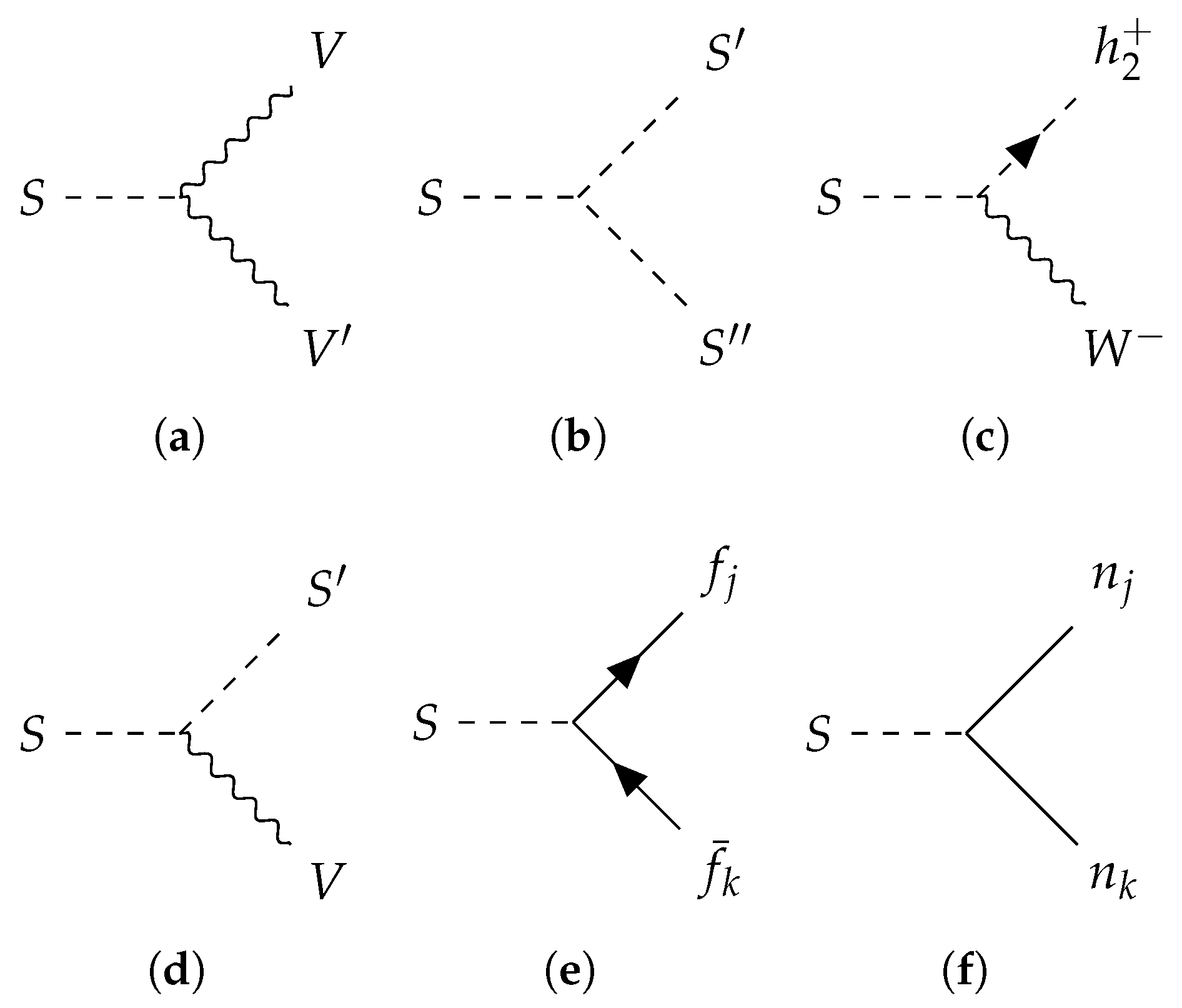
In this section we present all two-particle Higgs decays. The Feynman diagrams are pictured in Figure 1. Using the GNM Lagrangian in Equation (16), we express the amplitudes. Summing over spins or polarisations of the final state particles and using the phase space element in Appendix A, we write down the decay rates. Where applicable, we compare the results with the literature.

3.1. Higgs Decay into Gauge Bosons

Here we present the Higgs boson decays into gauge bosons. We construct the amplitude using Equations (1), (9), (17) and (19), and Figure 1. This amplitude is

$$i{\mathcal{M}}_{S\to V{V}^{\prime }}={\displaystyle \frac{1}{2}}i{g}_{V{V}^{\prime }}^{2}v{R}_{h_{1}S}{g}^{\mu \nu }{{ϵ}^{\ast }}^{\mu }\left(p_1\right){{ϵ}^{\ast }}^{\nu }\left(p_2\right),$$

(39)

where $S=h_0,H_0,A$ corresponds to the Higgs mass eigenstates, $V,V^{\prime }=\gamma ,W,Z$, and

$$g_{V{V}^{\prime }}=\left\{\begin{array}{cc}0,\hfill & \mathrm{if}V\mathrm{or}{V}^{\prime }=\gamma \hfill \\ g,\hfill & \mathrm{if}V=V^{\prime }=W\hfill \\ {\displaystyle \frac{g}{cos{\theta }_{\mathrm{W}}}},\hfill & \mathrm{if}V=V^{\prime }=Z\hfill \end{array}\right..$$

(40)

The momenta of the outgoing particles are $p_i$ with $i=1,2$.

To get the decay rate, we square this amplitude and sum over polarisations of the final state particles. Using the result for the phase space element in

Table A1. Table representing the value of the phase space element in a massless system, on with one massive particle and one with two particles with the same mass.

	${\mathit{m}}_1={\mathit{m}}_2=0$	${\mathit{m}}_1=0,{\mathit{m}}_2\ne 0$	${\mathit{m}}_1={\mathit{m}}_2=\mathit{m}$
${\Pi }_{\mathrm{LIPS}}$	${\displaystyle \frac{1}{8\pi }}$	${\displaystyle \frac{1}{4\pi }}{\displaystyle \frac{m_q^2-m_2^2}{2m_q^2}}$	${\displaystyle \frac{1}{8\pi }}\sqrt{1-{\displaystyle \frac{4m^2}{m_q^2}}}$

in Appendix A we write down the decay rate

$${\mathsf{\Gamma }}_{S\to V{V}^{\prime }}={\displaystyle \frac{g_{V{V}^{\prime }}^2{m}_S^3{R}_{h_{1}S}^2}{64\pi m_V^2}}{\lambda }_{SV}^{\prime }{f}_V,$$

(41)

where

$${\lambda }_{SV}^{\prime }=\sqrt{1-4x_{SV}}\left(1-4x_{SV}+12x_{SV}^2\right),$$

(42)

with $x_{SV}={\displaystyle \frac{m_V^2}{m_S^2}}$, and

$$f_V=\left\{\begin{array}{cc}{\displaystyle \frac{1}{2}},\hfill & \mathrm{if}V=Z\hfill \\ 1,\hfill & \mathrm{if}V=W\hfill \end{array}\right.,$$

(43)

is the statistical factor.

For CPC, i.e., $s_{13}=0$, and using $v={\displaystyle \frac{2m_W}{g}}$, the decay rates match the ones found in refs. [30,31]. For the decay $h_0\to WW$ of ref. [30], we have to identify their ${sin}^2(\alpha -\beta )$ with our $R_{h_{1}S}^2$. Taking our $R_{h_{1}S}^2$ and identifying it with ${cos}^2(\beta -\alpha )$ we get the decay rates that are equivalent to the ones in ref. [31]. In the case of $CP$ conservation, the pseudoscalar A does not decay into two gauge bosons at tree level. But the possible decay of $H_0$ into off-shell gauge bosons, with their subsequent decay into fermions, rules $H_0$ out as a possible dark matter candidate.

3.2. Higgs Decay into Lighter Higgses

The amplitudes for this decay are

$$i{\mathcal{M}}_{S\to S^{\prime }{S}^{″}}=-iv{\mathsf{\Xi }}_{S{S}^{\prime }{S}^{″}},$$

(44)

where

$$\begin{array}{cc}{\mathsf{\Xi }}_{S{S}^{\prime }{S}^{″}}\hfill & ={\displaystyle \frac{1}{v^2}}{R}_{h_{1}S}[({\delta }_{S^{\prime }{S}^{″}}-R_{h_1{S}^{\prime }}{R}_{h_1{S}^{″}})({\lambda }_3{v}^2-2m_{h_2^{+}}^2+m_{S^{\prime }}^2)+{\delta }_{S^{\prime }{S}^{″}}{m}_{S^{\prime }}^2]\hfill \\ \hfill & +\mathrm{Re}\left[{\lambda }_7{R}_S^{+}{R}_{S^{\prime }}^{+}{R}_{S^{″}}^{-}\right]+\mathrm{cyclic}\mathrm{permutations}\mathrm{of}\{S,S^{\prime },S^{″}\}.\hfill \end{array}$$

(45)

For this coupling we used the expressions for ${\lambda }_1$, ${\lambda }_4$, ${\lambda }_5$ and ${\lambda }_6$ from Appendix B. Using the result in Appendix A, Equation (A13), we write the decay rate

$${\mathsf{\Gamma }}_{S\to S^{\prime }{S}^{″}}={\displaystyle \frac{v^2{\mathsf{\Xi }}_{S{S}^{\prime }{S}^{″}}^2}{16\pi m_S^3}}\left(1-{\displaystyle \frac{{\delta }_{S^{\prime }{S}^{″}}}{2}}\right)\sqrt{{\left(m_S^2-m_{S^{\prime }}^2-m_{S^{″}}^2\right)}^2-4m_{S^{\prime }}^2{m}_{S^{″}}^2},$$

(46)

where $S\ne S^{\prime }{S}^{″}$ and the brackets with the Kronecker delta account for the statistical factor.

In CPC all $\lambda$s are real, and ${\lambda }_7=0$, and the mixing between the pseudoscalar A and the real scalars $h_0$ and $H_0$ vanishes, giving $R_{h_{1,2}A}=R_{h_3{h}_0}=R_{h_3{H}_0}=0$. Then ${\mathsf{\Xi }}_{A{S}^{\prime }{S}^{″}}$ vanishes and the pseudoscalar does not decay into the other Higgs bosons. For the scalar $H_0$, since it cannot decay into A, it leaves us with the coupling ${\mathsf{\Xi }}_{H_0{h}_0{h}_0}$, which is

$$\begin{array}{cc}\hfill {\mathsf{\Xi }}_{H_0{h}_0{h}_0}^{\mathrm{CPC}}& ={\displaystyle \frac{R_{h_1{H}_0}}{v^2}}[(1-3R_{h_1{h}_0}^2)({\lambda }_3{v}^2-2m_{h_2^{+}}^2)+(1-R_{h_1{h}_0}^2)2m_{h_0}^2-R_{h_1{h}_0}^2{m}_{H_0}^2]\hfill \\ & +\mathrm{Re}\left[{\lambda }_7{R}_{h_0}^{+}(2R_{H_0}^{+}{R}_{h_0}^{-}+R_{h_0}^{+}{R}_{H_0}^{-})\right].\hfill \end{array}$$

(47)

The GNM and IDM have similar coupling structures, but Higgs doublets do not mix in the IDM. To take the IDM limit for the GNM, in addition to the previous parameter choices for CPC, we also take $s_{12}=1$. Then the elements of matrix R in Equation (21) become

$$R=\left(\begin{array}{ccc}{R}_{h_1{h}_0}& R_{h_2{h}_0}& R_{h_3{h}_0}\\ R_{h_1{H}_0}& R_{h_2{H}_0}& R_{h_3{H}_0}\\ R_{h_{1}A}& R_{h_{2}A}& R_{h_{3}A}\end{array}\right)\to \left(\begin{array}{ccc}0& 1& 0\\ -1& 0& 0\\ 0& 0& 1\end{array}\right),$$

(48)

with

$$R_S^{\pm }=R_{h_{2}S}\pm i{R}_{h_{3}S}\to -{\delta }_{S{h}_0}\pm i{\delta }_{SA}.$$

(49)

The coupling in the IDM limit is

$${\mathsf{\Xi }}_{H_0{h}_0{h}_0}^{\mathrm{IDM}}={\lambda }_3+{\displaystyle \frac{2m_{h_0}^2-2m_{h_2^{+}}^2}{v^2}}={\lambda }_3+{\lambda }_4+2\mathrm{Re}\left[{\lambda }_5\right]=:{\lambda }_{345},$$

(50)

where the transformation laws in Appendix B give the second equality. In refs. [7,30] the factor of 2 in front of ${\lambda }_5$ in Equation (50) does not appear due to differing conventions in the potential in Equation (11).

In this limit the decay rate is

$${\mathsf{\Gamma }}_{H_0\to h_0{h}_0}^{\mathrm{IDM}\mathrm{limit}}={\displaystyle \frac{v^2{\left({\lambda }_{345}\right)}^2}{32\pi m_{H_0}}}\sqrt{1-{\displaystyle \frac{4m_{h_0}^2}{m_{H_0}^2}}},$$

(51)

which is equivalent to the one found in Ref. [7] (p. 188), except in the reference, the decay is with particles swapped, i.e., $h_0\to H_0{H}_0$.

3.3. Higgs Decay into a Charged Higgs and W Boson

If the neutral Higgs bosons are more massive than the charged Higgs boson, they can decay into it and a charged gauge boson. Using Equation (9) we read the amplitude for such a decay

$$i{\mathcal{M}}_{S\to W^{-}{h}_2^{+}}=i{\displaystyle \frac{g}{2}}{R}_S^{+}\left(p_1^{\mu }+q^{\mu }\right){ϵ}^{\ast \mu }\left(p_2^{\mu }\right).$$

(52)

Using the result of Equation (A13) in Appendix A for the general phase space element, we write down the decay rate as

$${\mathsf{\Gamma }}_{S\to W^{-}{h}_2^{+}}={\displaystyle \frac{g^2}{64\pi m_W^2{m}_S^3}}{R}_S^{+}{R}_S^{-}{\left({\left(m_S^2-m_W^2-m_{h_2^{+}}^2\right)}^2-4m_W^2{m}_{h_2^{+}}^2\right)}^{3/2}.$$

(53)

In the $CP$ conserving case the $H_0$ decay becomes equivalent to the one found in [31].

3.4. Higgs Decay into a Neutral Higgs and Z Boson

If one of the neutral Higgs bosons is more massive than the other neutral Higgses, it can decay into a neutral Higgs and a Z boson. Using Equation (9) we read the amplitude for this process:

$$i{\mathcal{M}}_{S\to S^{\prime }Z}={\displaystyle \frac{g}{2cos{\theta }_{\mathrm{W}}}}\mathrm{Im}\left[R_S^{+}{R}_{S^{\prime }}^{-}\right]\left(p_1^{\mu }+q^{\mu }\right){ϵ}^{\ast \mu },$$

(54)

As we did in the previous section, we use the general phase space element, Equation (A13), to write down the decay rate:

$${\mathsf{\Gamma }}_{S\to S^{\prime }Z}={\displaystyle \frac{g^2}{64\pi m_S^3{m}_Z^2{cos}^2{\theta }_{\mathrm{W}}}}{\left(\mathrm{Im}\left[R_S^{+}{R}_{S^{\prime }}^{-}\right]\right)}^2{\left({\left(m_S^2-m_{S^{\prime }}^2-m_Z^2\right)}^2-4m_Z^2{m}_{S^{\prime }}^2\right)}^{3/2},$$

(55)

where $S\ne S^{\prime }$. This decay rate is equivalent to those found in refs. [30,31].

3.5. Higgs Decay into Charged Fermions

Here we present Higgs decays into charged fermions. For these decays we take the fermions in the final state phase space to be massless, since their masses are much smaller than the mass of the decaying Higgs. (Our calculations do not include top quarks, as they are too heavy.)

For the decay of Figure 1e, the sum of the Yukawa couplings, Equation (14),

$${\left({\mathcal{A}}_F\right)}_{jk}=R_{h_{1}S}{\left(Y_F^{\left(1\right)}\right)}_{jk}+R_S^{-}{\left(Y_F^{\left(2\right)}\right)}_{jk},$$

(56)

gives the amplitude

$$i{\mathcal{M}}_{S\to {\ell }_j{\ell }_k}={\displaystyle \frac{i}{\sqrt{2}}}{\overline{u}}_j\left[{\left({\mathcal{A}}_F\right)}_{jk}{P}_L+{\left({\mathcal{A}}_F^{†}\right)}_{jk}{P}_R\right]v_k.$$

(57)

The decay rate is then

$$\begin{array}{cc}\hfill {\mathsf{\Gamma }}_{S\to {\ell }_j{\ell }_k}& ={\displaystyle \frac{m_S}{32\pi }}\left(|{\left({\mathcal{A}}_F\right)}_{jk}{|}^2+{\left|{\left({\mathcal{A}}_F\right)}_{kj}\right|}^2\right)\hfill \\ \hfill & ={\displaystyle \frac{m_S}{32\pi }}({\delta }_{jk}{R}_{h_{1}S}^2{\displaystyle \frac{4m_j^2}{v^2}}+{\delta }_{jk}{R}_{h_{1}S}{\displaystyle \frac{4\sqrt{2}{m}_j}{v}}\mathrm{Re}\left[R_S^{-}{\left(Y_F^{\left(2\right)}\right)}_{jk}\right]\hfill \\ & +R_S^{+}{R}_S^{-}\left(|{\left(Y_F^{\left(2\right)}\right)}_{jk}{|}^2+{\left|{\left(Y_F^{\left(2\right)}\right)}_{kj}\right|}^2\right)).\hfill \end{array}$$

(58)

The first term comes from the first Higgs doublet, while the others come because of the second Higgs doublet.

Taking only the term coming from the first Higgs doublet, setting $S=h_0$ and $R_{h_1{h}_0}=1$, and using Equation (24), we get that the decay rate simplifies to the SM Higgs decay rate

$${\mathsf{\Gamma }}_{h_0\to {\ell }_j{\ell }_j}^{\mathrm{SM}}={\displaystyle \frac{m_{h_0}{m}_j^2}{8\pi v^2}},$$

(59)

which can be found in the literature, e.g., ref. [31].

For non-diagonal lepton Yukawa couplings $Y_{F=L}^{\left(2\right)}$, the decays, Equation (58), also include charged lepton flavour-violating (cLFV) currents. Current or upcoming experiments [41,42,43] work to limit the size of the non-diagonal lepton Yukawa couplings. But since these cLFV decays have a different final state than the neutrino decays discussed in the following section, they can only increase the decay rate and hence will not contribute to the lower limit that comes from the non-vanishing neutrino Yukawa couplings.

3.6. Higgs Decay into Two Neutrinos

For the kinematics we take the active neutrinos to be massless in the phase space of the final state. The sum of the Yukawa couplings Equation (14)

$${\left({\mathcal{A}}_N\right)}_{jk}=R_{h_{1}S}{(U_L^T·Y_N^{\left(1\right)}·U_R^{\ast })}_{jk}+R_S^{+}{(U_L^T·Y_N^{\left(2\right)}·U_R^{\ast })}_{jk},$$

(60)

has to be symmetrised and gives the general amplitude for these decays:

$$i{\mathcal{M}}_{S\to n_j{n}_k}=-{\displaystyle \frac{i}{\sqrt{2}}}{\overline{u}}_j\left[{\left({\mathcal{A}}_N\right)}_{jk}{P}_L+{\left({\mathcal{A}}_N\right)}_{kj}{P}_L+{\left({\mathcal{A}}_N^{†}\right)}_{jk}{P}_R+{\left({\mathcal{A}}_N^{†}\right)}_{kj}{P}_R\right]v_k.$$

(61)

With the splitting of U into $U_L$ and $U_R$, the amplitude ${\mathcal{A}}_N$ also splits into a direct product of the two vectors $(U_L^T·Y_N)$ and $U_R$. We can easily see

$$U_L^T·{\overrightarrow{\mathrm{v}}}_j={\left(\begin{array}{cccc}{\overrightarrow{\mathrm{v}}}_1^{\ast }& {\overrightarrow{\mathrm{v}}}_2^{\ast }& c{\overrightarrow{\mathrm{v}}}_3^{\ast }& is{\overrightarrow{\mathrm{v}}}_3^{\ast }\end{array}\right)}^T·{\overrightarrow{\mathrm{v}}}_j={\left(\begin{array}{cccc}{\delta }_{j1}& {\delta }_{j2}& c{\delta }_{j3}& is{\delta }_{j3}\end{array}\right)}^T,$$

(62)

which gives the simplifying relations

$$\begin{array}{c}\hfill U_L^T·{\overrightarrow{Y}}_N^{\left(1\right)}=U_L^T·(-iy{\overrightarrow{\mathrm{v}}}_3)=-iy{\left(\begin{array}{cccc}0& 0& c& is\end{array}\right)}^T,\end{array}$$

(63)

and

$$\begin{array}{c}\hfill U_L^T·{\overrightarrow{Y}}_N^{\left(2\right)}=U_L^T·(d{\overrightarrow{\mathrm{v}}}_2+d^{\prime }{\overrightarrow{\mathrm{v}}}_3)={\left(\begin{array}{cccc}0& d& c{d}^{\prime }& is{d}^{\prime }\end{array}\right)}^T.\end{array}$$

(64)

With the abbreviations

$$\begin{array}{c}\hfill B_S^{+}=y{R}_{h_{1}S}+i{d}^{\prime }{R}_S^{+}\mathrm{and}{B}_S^{-}=y{R}_{h_{1}S}-i{d}^{\prime \ast }{R}_S^{-}\end{array}$$

(65)

we can write ${\mathcal{A}}_N$ in matrix form as

$$\begin{array}{cc}\hfill {\left({\mathcal{A}}_N\right)}_{jk}& ={\left(0d{R}_S^{+}-ic{B}_S^{+}s{B}_S^{+}\right)}_j^T{\left(00isc\right)}_k\hfill \\ \hfill & =[d{R}_S^{+}{\delta }_{j2}+B_S^{+}(s{\delta }_{j4}-ic{\delta }_{j3})](is{\delta }_{k3}+c{\delta }_{k4}).\hfill \end{array}$$

(66)

The symmetrisation in $\left(jk\right)$ then gives the index structure

$$2{\left({\mathcal{A}}_N\right)}_{\left(jk\right)}=d{R}_S^{+}(is{\Delta }_{jk}^{23}+c{\Delta }_{jk}^{24})+B_S^{+}(sc({\Delta }_{jk}^{33}+{\Delta }_{jk}^{44})-i(c^2-s^2){\Delta }_{jk}^{34}),$$

(67)

where

$${\Delta }_{jk}^{\ell m}={\delta }_{j\ell }{\delta }_{km}+{\delta }_{jm}{\delta }_{k\ell }.$$

(68)

From this amplitude we see that the Higgs bosons will decay into these five final states: $n_2{n}_3$, $n_2{n}_4$, $n_3{n}_3$, $n_3{n}_4$, and $n_4{n}_4$. These decay rates are:

$${\mathsf{\Gamma }}_{S\to n_2{n}_3}={\displaystyle \frac{1}{2m_S}}{\displaystyle \frac{1}{8\pi }}{\displaystyle \frac{1}{2}}{m}_S^{2}2{\left|2{\left({\mathcal{A}}_N\right)}_{\left(23\right)}\right|}^2={\displaystyle \frac{m_S}{16\pi }}{s}^2{d}^2{R}_S^{+}{R}_S^{-},$$

(69)

$${\mathsf{\Gamma }}_{S\to n_2{n}_4}={\displaystyle \frac{{(m_S^2-m_4^2)}^2}{32\pi m_S^3}}2{\left|2{\left({\mathcal{A}}_N\right)}_{\left(24\right)}\right|}^2={\displaystyle \frac{{(m_S^2-m_4^2)}^2}{16\pi m_S^3}}{c}^2{d}^2{R}_S^{+}{R}_S^{-},$$

(70)

$${\mathsf{\Gamma }}_{S\to n_3{n}_3}={\displaystyle \frac{m_S}{32\pi }}|2{\left({\mathcal{A}}_N\right)}_{\left(33\right)}{|}^2={\displaystyle \frac{m_S}{32\pi }}4s^2{c}^2{\left|B_S^{+}\right|}^2,$$

(71)

$${\mathsf{\Gamma }}_{S\to n_3{n}_4}={\displaystyle \frac{{(m_S^2-m_4^2)}^2}{32\pi m_S^3}}2|2{\left({\mathcal{A}}_N\right)}_{\left(34\right)}{|}^2={\displaystyle \frac{{(m_S^2-m_4^2)}^2}{16\pi m_S^3}}{(c^2-s^2)}^2{\left|B_S^{+}\right|}^2,$$

(72)

$$\begin{array}{cc}\hfill {\mathsf{\Gamma }}_{S\to n_4{n}_4}& ={\displaystyle \frac{\sqrt{m_S^2-4m_4^2}}{64\pi m_S^2}}\left[(m_S^2-2m_4^2)2{\left|2{\left({\mathcal{A}}_N\right)}_{\left(44\right)}\right|}^2-2m_4^2[2{\left({\mathcal{A}}_N\right)}_{\left(44\right)}^2+2{\left({\mathcal{A}}_N^{\ast }\right)}_{\left(44\right)}^2]\right]\hfill \\ \hfill & ={\displaystyle \frac{\sqrt{m_S^2-4m_4^2}}{8\pi m_S^2}}{s}^2{c}^2\left[(m_S^2-2m_4^2){\left|B_S^{+}\right|}^2-2m_4^2\mathrm{Re}\left[B_S^{+2}\right]\right],\hfill \end{array}$$

(73)

with

$$|B_S^{+}{|}^2=B_S^{+}{B}_S^{-}=y^2{R}_{h_{1}S}^2-2y{R}_{h_{1}S}\mathrm{Im}\left[d^{\prime }{R}_S^{+}\right]+{\left|d^{\prime }\right|}^2{R}_S^{+}{R}_S^{-},$$

(74)

and

$$\mathrm{Re}\left[B_S^{+2}\right]=\mathrm{Re}[y^2{R}_{h_{1}S}^2+2iy{R}_{h_{1}S}{d}^{\prime }{R}_S^{+}-d^{\prime 2}{\left(R_S^{+}\right)}^2]={\left|B_S^{+}\right|}^2-2{\left(\mathrm{Re}\left[d^{\prime }{R}_S^{+}\right]\right)}^2.$$

(75)

4. Scalar Dark Matter Candidates in the GNM

The IDM is treated in the literature [6,22,44,45] as one of the simplest extensions of the SM that can provide a DM candidate. The stability of this candidate hinges on an unbroken symmetry, usually a $Z_2$, but sometimes also a $U{\left(1\right)}_{\mathrm{Peccei}\mathrm{Quinn}}$ [46], that prevents the decay. Ref. [6] connects the IDM to neutrino physics and presents the dependence of the neutrino masses on the ${\lambda }_5$ parameter of the Higgs potential—Equation (11). Ref. [47] explains the smallness of ${\lambda }_5$ as technical naturalness, as the vanishing of ${\lambda }_5$ enhances the symmetry of the model. Ref. [14] extends this concept to define the tiny seesaw regime of the GNM, where not only ${\lambda }_5$, but also the $Z_2$-violating neutrino Yukawa couplings are taken to be technically natural, i.e., very small, since their absence enhances the symmetry of the model. As the IDM relies on the protective $Z_2$ symmetry it does not contain these Yukawa couplings, that are needed for the neutrino mass generation. When comparing the GNM to the IDM we ask whether the pseudoscalar A of the GNM behaves like the DM candidate of the IDM in the limit where both models appear most similar. This requires us to take the CPC limit, described in Section 3.2, to take ${\lambda }_6\to 0$, to restrict the Higgs mixing matrix R, as described in Equation (48), and to take the charged fermion Yukawa couplings to the second Higgs doublet as vanishing.

Setting ${\lambda }_{6,7}\to 0$, which is required by the $Z_2$ symmetry of the IDM, and using Equation (48) simplifies

$$R_S^{+}{R}_S^{-}\to 1-{\delta }_{S{h}_0}={\delta }_{S{H}_0}+{\delta }_{SA},\mathrm{and}{B}_S^{+}\to (y-id){\delta }_{S{h}_0}-d^{\prime }{\delta }_{SA},$$

(76)

giving the decay rate to the light neutrinos as

$${\mathsf{\Gamma }}_{A\to 2\nu }^{\mathrm{IDM}\mathrm{limit}}={\displaystyle \frac{m_A{s}^2(d^2+2c^2|d^{\prime }{|}^2)}{16\pi }}.$$

(77)

The requirement of the GNM to give one neutrino a seesaw mass and another a radiative mass breaks the protective symmetries of the IDM: assigning N to be odd under $Z_2$ forbids $Y_N^{\left(1\right)}$, which is needed for the seesaw. For the radiative mass we need the self-energy function defined in [14] in terms of the Passarino–Veltman functions [48] and the conventions of [49]

$$\Lambda ={\displaystyle \frac{m_4}{32{\pi }^2}}\left[B_0(0,m_4^2,m_A^2)-B_0(0,m_4^2,m_{H_0}^2)\right],$$

(78)

which is proportional to the radiative mass and hence required to be non-zero. It is directly proportional to $m_A^2-m_{H_0}^2\propto {\lambda }_5$ which breaks the Peccei–Quinn symmetry that the Higgs potential has in the case of ${\lambda }_5\to 0$. As a result we have Yukawa couplings in the GNM that break $Z_2$ and depend on ${\lambda }_5\ne 0$. An exact parametrisation of these couplings, depending on the free parameters of the model, useful in the context of lepton flavour violation, can be found in [14]. Using only d and $|d^{\prime }|$ is enough for our case. Obviously $|d^{\prime }| \ge 0$, and

$$d^2={\displaystyle \frac{m_2^{\mathrm{pole}}{m}_3^{\mathrm{pole}}}{m_3\left|\Lambda \right|}},$$

(79)

which can be seen by taking the determinant of Equation (2.19) of [14], where $m_3$ denotes the seesaw mass, that comes from the coupling relation in Equation (34). From Equation (31) we see that $s^2\approx {\displaystyle \frac{m_3}{m_4}}$, which gives the simplified lower limit for the decay rate:

$${\mathsf{\Gamma }}_{A\to 2\nu }^{\mathrm{IDM}\mathrm{limit}}\ge {\displaystyle \frac{m_A{s}^2{d}^2}{16\pi }}={\displaystyle \frac{m_A{m}_2^{\mathrm{pole}}{m}_3^{\mathrm{pole}}}{16\pi m_4\left|\Lambda \right|}}=:{\mathsf{\Gamma }}_{\left(m_4\right)}^{\mathrm{limit}}.$$

(80)

So an upper bound on $\left|\Lambda \right|$ in the considered parameter range of $m_4$, $m_A$, and $m_{H_0}$ gives us an upper bound on the lifetime of our IDM-like dark matter candidate.

The functional dependence is more clear if we write the $B_0$ functions in $\Lambda$ explicitly in terms of the squared mass ratios $x=m_4^2/m_A^2$ and $y=m_4^2/m_{H_0}^2$; therefore,

$$\Lambda ={\displaystyle \frac{m_4}{32{\pi }^2}}\left({\displaystyle \frac{lnx}{1-x}}-{\displaystyle \frac{lny}{1-y}}\right).$$

(81)

Upon inserting this form into Equation (80) we get

$${\mathsf{\Gamma }}_{\left(m_4\right)}^{\mathrm{limit}}={\displaystyle \frac{2\pi m_A{m}_2^{\mathrm{pole}}{m}_3^{\mathrm{pole}}}{m_4^2}}|{\displaystyle \frac{lnx}{1-x}}-{\displaystyle \frac{lny}{1-y}}{|}^{-1},$$

(82)

so that there is a an overall prefactor of $m_4^{-2}$ and logarithmic dependence on the squared mass ratios.

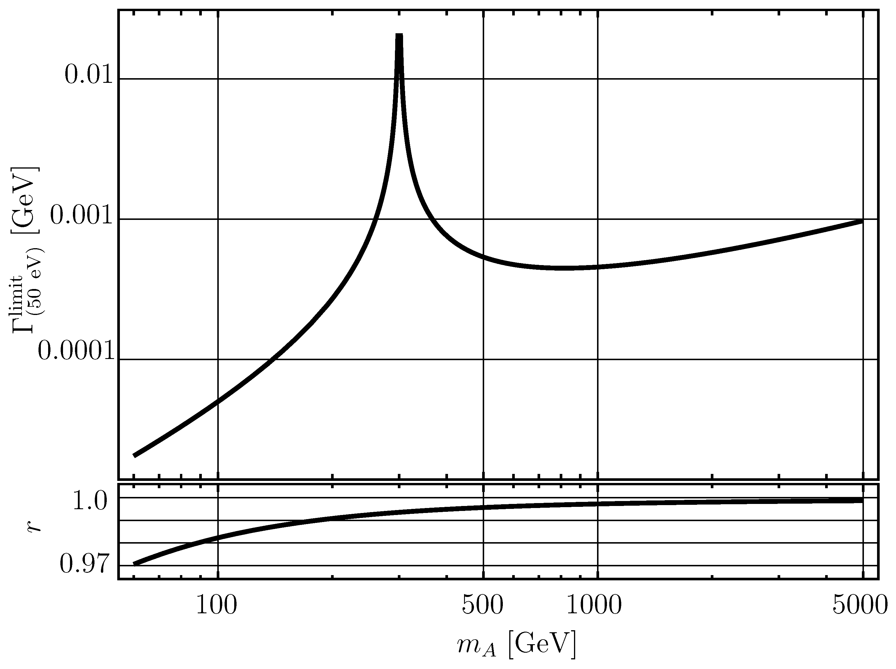
We present the dependence of our decay rate bound on $m_A$, taking a more conservative value for $m_{H_0}=300\mathrm{GeV}$ and the lower limit of the tiny seesaw scale with $m_4=50\mathrm{eV}$ in Figure 2. As a sanity check we plot the decay rate up to rather high values of $m_A$ to show the eventual increase of the decay rate with increasing mass of the pseudoscalar A, thus escaping the counterintuitive region right above $m_A=m_H$, where we observe an opposite effect. The upper limit of the tiny seesaw scale with $m_4=10\mathrm{GeV}$ is presented in the lower pane of the same figure through the ratio

$$r={\displaystyle \frac{{\mathsf{\Gamma }}_{\left(50\mathrm{eV}\right)}^{\mathrm{limit}}}{{\mathsf{\Gamma }}_{\left(10\mathrm{GeV}\right)}^{\mathrm{limit}}}}\times {\displaystyle \frac{{\left(50\mathrm{eV}\right)}^2}{{\left(10\mathrm{GeV}\right)}^2}},$$

(83)

where ${\left(10\mathrm{GeV}\right)}^2/{\left(50\mathrm{eV}\right)}^2=4\times {10}^{16}$ cancels the explicit quadratic dependence on $m_4$ in Equation (82). The ratio r then isolates and compares the logarithmic dependence for different values of $m_4$. The lower pane of Figure 2 shows that the decay rates in the lower and upper limits of the tiny seesaw regime, except for the overall scale, slightly differ for lower values of $m_A$, where the squared mass ratio x is important. At the lower end of $m_A=60\mathrm{GeV}$, the squared mass ratio for $m_4=50\mathrm{eV}$ is $x\approx 0$, and for $m_4=10\mathrm{GeV}$ we have $x\approx 0.028$, which eventually translates into $r\approx 0.97$. For high values of $m_A$, the ratio x becomes negligible for all considered values of $m_4$ and brings the ratio $r\to 1$, provided the ratio y is also negligible for the considered values of $m_4$.

Taking the extreme value $m_4=10\mathrm{TeV}$, which is far outside the tiny seesaw regime, but seems to be the upper limit of perturbativity of the model, as suggested by private studies with FlexibleSUSY [50,51], and taking $m_A=60\mathrm{GeV}$ and $m_{H_0}=800\mathrm{GeV}$, we get an upper limit of the lifetime of our IDM-like dark matter candidate of 13 seconds, which excludes it as a real dark matter candidate. In the region where this model stays perturbative we expect this limit to also hold beyond tree level. In the case of an inverted hierarchy of neutrino masses, our obtained limit for the decay rate becomes $5.6$ times larger due to the increase in the neutrino pole masses. In addition, in

Table 1. The upper limit of the lifetime of the pseudoscalar A, when the scalar $H_0$ mass is $m_{H_0}=300\mathrm{GeV}$. Rows correspond to different choices of $m_4$ and columns to different choices of $m_A$. The fourth row with $m_4=10\mathrm{TeV}$ is no longer in the tiny seesaw regime.

	$m_A=60\mathrm{GeV}$	$m_A=250\mathrm{GeV}$	$m_A=500\mathrm{GeV}$
$m_4=50\mathrm{eV}$	$3.22·{10}^{-20}\mathrm{s}$	$8.75·{10}^{-22}\mathrm{s}$	$1.23·{10}^{-21}\mathrm{s}$
$m_4=1\mathrm{keV}$	$1.29·{10}^{-17}\mathrm{s}$	$3.50·{10}^{-19}\mathrm{s}$	$4.90·{10}^{-19}\mathrm{s}$
$m_4=10\mathrm{GeV}$	$1.25·{10}^{-3}\mathrm{s}$	$3.47·{10}^{-5}\mathrm{s}$	$4.88·{10}^{-5}\mathrm{s}$
$m_4=10\mathrm{TeV}$	$2.38\mathrm{s}$	$0.16\mathrm{s}$	$0.42\mathrm{s}$

and

Table 2. The upper limit of the lifetime for the pseudoscalar A, when the scalar $H_0$ mass is $m_{H_0}=800\mathrm{GeV}$. Rows correspond to different choices of $m_4$ and columns to different choices of $m_A$. The fourth row with $m_4=10\mathrm{TeV}$ is no longer in the tiny seesaw regime.

	$m_A=60\mathrm{GeV}$	$m_A=250\mathrm{GeV}$	$m_A=500\mathrm{GeV}$
$m_4=50\mathrm{eV}$	$5.18·{10}^{-20}\mathrm{s}$	$5.59·{10}^{-21}\mathrm{s}$	$1.13·{10}^{-21}\mathrm{s}$
$m_4=1\mathrm{keV}$	$2.07·{10}^{-17}\mathrm{s}$	$2.23·{10}^{-18}\mathrm{s}$	$4.51·{10}^{-19}\mathrm{s}$
$m_4=10\mathrm{GeV}$	$2.03·{10}^{-3}\mathrm{s}$	$2.22·{10}^{-4}\mathrm{s}$	$4.50·{10}^{-5}\mathrm{s}$
$m_4=10\mathrm{TeV}$	$12.87\mathrm{s}$	$2.68\mathrm{s}$	$0.84\mathrm{s}$

we provide the upper limits of the lifetime of the pseudoscalar A for selected values of $m_{H_0}$, $m_A$, and $m_4$.

5. Conclusions

In this paper we have calculated the contributions of tree level processes with two particles in the final state to the decay rates of the Grimus–Neufeld model scalar bosons. The decays into gauge bosons and other bosons match the ones found in the literature, for example, refs. [30,31]. The general form of the decay amplitude into Higgses, Equations (44) and (45), seems to be new, but all special cases that we could find in the literature also match—as an example, see [7]. In principle this general decay amplitude can allow the determination of the free parameters ${\lambda }_3$ and ${\lambda }_7$ of the Higgs potential, if the corresponding decays can be measured.

The decay rate formula into charged leptons, Equation (58), shows that lepton flavour-violating decays are directly proportional to the entries in the second Higgs doublet’s Yukawa coupling and that no cancellation of different entries can occur.

The decay amplitude to neutrinos is more complicated due to their Majorana nature. The simple structure in Equation (67) shows that the lightest massless neutrino state does not couple to the Higgs bosons and stresses the importance of second Higgs doublet couplings to the active neutrinos. These couplings give a lower bound on the decay rates of the GNM scalars, see Equations (69), (71) and (80). From Equation (80) one sees the proportionality of this lower bound to the masses of the light neutrinos and the breaking of the $U{\left(1\right)}_{\mathrm{Peccei}\mathrm{Quinn}}$, as discussed below Equation (78). This result is valid for any scale, because the symmetry breaking is required for the neutrino masses. Thus the limit obtained in this paper is independent and complimentary to collider and astrophysical bounds.

The IDM and the scoto-seesaw model [12] have very similar coupling structures to our GNM, especially with respect to lepton flavour-violating observables—see [14]. Both the IDM and the scoto-seesaw model have a scalar DM candidate. These candidates are stable due to a protective symmetry, which is softly broken in the GNM. The lower bound for the decay rate excludes the GNM scalar dark matter candidate. In this aspect the slight symmetry breaking required in the GNM is enough to have a large phenomenological impact.

References

1. The CMS collaboration. Stairway to Discovery: A Report on the CMS Programme of Cross Section Measurements from Millibarns to Femtobarns. Phys. Rep. 2025, 1115, 3–115. [Google Scholar] [CrossRef] [Scilit]
2. The ATLAS Collaboration. Standard Model Summary Plots June 2024; Technical Report; CERN: Geneva, Switzerland, 2024. [Google Scholar]
3. Fukuda, Y.; Hayakawa, T.; Ichihara, E.; Inoue, K.; Ishihara, K.; Ishino, H.; Itow, Y.; Kajita, T.; Kameda, J.; Kasuga, S.; et al. Evidence for Oscillation of Atmospheric Neutrinos. Phys. Rev. Lett. 1998, 81, 1562–1567. [Google Scholar] [CrossRef] [Scilit]
4. Cirelli, M.; Strumia, A.; Zupan, J. Dark Matter. Scipost Phys. Rev. 2026, 1, 689. [Google Scholar] [CrossRef] [Scilit]
5. Deshpande, N.G.; Ma, E. Pattern of Symmetry Breaking with Two Higgs Doublets. Phys. Rev. D 1978, 18, 2574. [Google Scholar] [CrossRef] [Scilit]
6. Ma, E. Verifiable Radiative Seesaw Mechanism of ν Mass and Dark Matter. Phys. Rev. D 2006, 73, 077301. [Google Scholar] [CrossRef] [Scilit]
7. Krawczyk, M.; Darvishi, N.; Sokołowska, D. The Inert Doublet Model and Its Extensions. Acta Phys. Pol. B 2016, 47, 183. [Google Scholar] [CrossRef] [Scilit]
8. Dodelson, S.; Widrow, L.M. Sterile Neutrinos as Dark Matter. Phys. Rev. Lett. 1994, 72, 17–20. [Google Scholar] [CrossRef] [Scilit] [PubMed]
9. Ghiglieri, J.; Laine, M. Improved Determination of Sterile Neutrino Dark Matter Spectrum. J. High Energy Phys. 2015, 2015, 171. [Google Scholar] [CrossRef] [Scilit]
10. Drewes, M.; Kang, J.U. Sterile Neutrino Dark Matter Production from Scalar Decay in a Thermal Bath. J. High Energy Phys. 2016, 2016, 51. [Google Scholar] [CrossRef] [Scilit]
11. Boyarsky, A.; Drewes, M.; Lasserre, T.; Mertens, S.; Ruchayskiy, O. Sterile Neutrino Dark Matter. Prog. Part. Nucl. Phys. 2019, 104, 1–45. [Google Scholar] [CrossRef] [Scilit]
12. Rojas, N.; Srivastava, R.; Valle, J.W.F. Simplest Scoto-Seesaw Mechanism. Phys. Lett. B 2019, 789, 132–136. [Google Scholar] [CrossRef] [Scilit]
13. Grimus, W.; Neufeld, H. Radiative Neutrino Masses in an SU(2) × U(1) Model. Nucl. Phys. B 1989, 325, 18–32. [Google Scholar] [CrossRef] [Scilit]
14. Dūdėnas, V.; Gajdosik, T.; Khasianevich, U.; Kotlarski, W.; Stöckinger, D. Charged Lepton Flavor Violating Processes in the Grimus-Neufeld Model. J. High Energy Phys. 2022, 2022, 174. [Google Scholar] [CrossRef] [Scilit]
15. Draukšas, S. Renormalization of the Grimus-Neufeld Model. Ph.D. Thesis, Vilnius University, Vilnius, Lithuania, 2024. [Google Scholar] [CrossRef] [Scilit]
16. Mohapatra, R.N.; Senjanović, G. Neutrino Mass and Spontaneous Parity Nonconservation. Phys. Rev. Lett. 1980, 44, 912–915. [Google Scholar] [CrossRef] [Scilit]
17. Schechter, J.; Valle, J.W.F. Neutrino Decay and Spontaneous Violation of Lepton Number. Phys. Rev. D 1982, 25, 774–783. [Google Scholar] [CrossRef] [Scilit]
18. Giganti, C.; Lavignac, S.; Zito, M. Neutrino Oscillations: The Rise of the PMNS Paradigm. Prog. Part. Nucl. Phys. 2018, 98, 1–54. [Google Scholar] [CrossRef] [Scilit]
19. Arhrib, A.; Benbrik, R.; Gaur, N. Hγ gamma in the Inert Higgs Doublet Model. Phys. Rev. D 2012, 85, 095021. [Google Scholar] [CrossRef] [Scilit]
20. Świeżewska, B.; Krawczyk, M. Diphoton Rate in the Inert Doublet Model with a 125 GeV Higgs Boson. Phys. Rev. D 2013, 88, 035019. [Google Scholar] [CrossRef] [Scilit]
21. Díaz, M.A.; Koch, B.; Urrutia-Quiroga, S. Constraints to Dark Matter from Inert Higgs Doublet Model. Adv. High Energy Phys. 2016, 2016, 1–9. [Google Scholar] [CrossRef] [Scilit]
22. Belyaev, A.; Cacciapaglia, G.; Ivanov, I.P.; Rojas-Abatte, F.; Thomas, M. Anatomy of the Inert Two-Higgs-doublet Model in the Light of the LHC and Non-LHC Dark Matter Searches. Phys. Rev. D 2018, 97, 035011. [Google Scholar] [CrossRef] [Scilit]
23. The CMS collaboration; Sirunyan, A.M.; Tumasyan, A.; Adam, W.; Andrejkovic, J.W.; Bergauer, T.; Chatterjee, S.; Dragicevic, M.; Escalante Del Valle, A.; Frühwirth, R.; et al. Measurements of Higgs Boson Production Cross Sections and Couplings in the Diphoton Decay Channel at s = 13 TeV. J. High Energy Phys. 2021, 2021, 27. [Google Scholar] [CrossRef] [Scilit]
24. The ATLAS collaboration; Aad, G.; Abbott, B.; Abbott, D.C.; Abeling, K.; Abidi, S.H.; Aboulhorma, A.; Abramowicz, H.; Abreu, H.; Abulaiti, Y.; et al. Measurement of the Properties of Higgs Boson Production at s = 13 TeV in the Hγγ Channel Using 139 fb−1 of pp Collision Data with the ATLAS Experiment. J. High Energy Phys. 2023, 2023, 88. [Google Scholar] [CrossRef] [Scilit]
25. El Kaffas, A.W.; Khater, W.; Magne Ogreid, O.; Osland, P. Consistency of the Two-Higgs-doublet Model and CP Violation in Top Production at the LHC. Nucl. Phys. B 2007, 775, 45–77. [Google Scholar] [CrossRef] [Scilit]
26. Grimus, W.; Lavoura, L.; Ogreid, O.M.; Osland, P. A Precision Constraint on Multi-Higgs-doublet Models. J. Phys. Nucl. Part. Phys. 2008, 35, 075001. [Google Scholar] [CrossRef] [Scilit]
27. Navas, S.; Amsler, C.; Gutsche, T.; Hanhart, C.; Hernández-Rey, J.J.; Lourenço, C.; Masoni, A.; Mikhasenko, M.; Mitchell, R.E.; Patrignani, C.; et al. Review of Particle Physics. Phys. Rev. D 2024, 110, 030001. [Google Scholar] [CrossRef] [Scilit]
28. Romao, J.C.; Silva, J.P. A Resource for Signs and Feynman Diagrams of the Standard Model. Int. J. Mod. Phys. A 2012, 27, 1230025. [Google Scholar] [CrossRef] [Scilit]
29. Alloul, A.; Christensen, N.D.; Degrande, C.; Duhr, C.; Fuks, B. FeynRules 2.0—A Complete Toolbox for tree level Phenomenology. Comput. Phys. Commun. 2014, 185, 2250–2300. [Google Scholar] [CrossRef] [Scilit]
30. Branco, G.C.; Ferreira, P.M.; Lavoura, L.; Rebelo, M.N.; Sher, M.; Silva, J.P. Theory and Phenomenology of Two-Higgs-doublet Models. Phys. Rep. 2012, 516, 1–102. [Google Scholar] [CrossRef] [Scilit]
31. Gunion, J.F.; Haber, H.E.; Kane, G.; Sally, D. The Higgs Hunter’s Guide, 1st ed.; CRC Press: Boca Raton, FL, USA, 2018. [Google Scholar] [CrossRef] [Scilit]
32. Haber, H.E.; O’Neil, D. Basis-Independent Methods for the Two-Higgs-doublet Model III: The CP-conserving Limit, Custodial Symmetry, and the Oblique Parameters S, T, U. Phys. Rev. D 2011, 83, 055017. [Google Scholar] [CrossRef] [Scilit]
33. Pal, P.B. Dirac, Majorana and Weyl Fermions. Am. J. Phys. 2011, 79, 485–498. [Google Scholar] [CrossRef] [Scilit]
34. Degrande, C. Automatic Evaluation of UV and R2 Terms for beyond the Standard Model Lagrangians: A Proof-of-Principle. Comput. Phys. Commun. 2015, 197, 239–262. [Google Scholar] [CrossRef] [Scilit]
35. Haber, H.E.; O’Neil, D. Basis-Independent Methods for the Two-Higgs-doublet Model II. The Significance of Tan(Beta). Phys. Rev. D 2006, 74, 015018. [Google Scholar] [CrossRef] [Scilit]
36. Takagi, T. On an Algebraic Problem Reluted to an Analytic Theorem of Carathéodory and Fejér and on an Allied Theorem of Landau. Jpn. J. Math. Trans. Abstr. 1924, 1, 83–93. [Google Scholar] [CrossRef] [Scilit] [PubMed]
37. Grimus, W.; Lavoura, L. Softly Broken Lepton Numbers and Maximal Neutrino Mixing. J. High Energy Phys. 2001, 2001, 45. [Google Scholar] [CrossRef] [Scilit]
38. Pontecorvo, B. Inverse Beta Processes and Nonconservation of Lepton Charge. Sov. Phys.–JETP [Zhurnal Eksperimentalnoi i Teoreticheskoi Fiziki] 1958, 7, 172–173. [Google Scholar]
39. Maki, Z.; Nakagawa, M.; Sakata, S. Remarks on the Unified Model of Elementary Particles. Prog. Theor. Phys. 1962, 28, 870–880. [Google Scholar] [CrossRef] [Scilit]
40. Dūdėnas, V.; Gajdosik, T.; Juodagalvis, A.; Jurčiukonis, D. The One-loop Improved Lagrangian of the Grimus-Neufeld Model. Acta Phys. Pol. B 2017, 48, 2235. [Google Scholar] [CrossRef] [Scilit]
41. Cirigliano, V.; Fuyuto, K.; Lee, C.; Mereghetti, E.; Yan, B. Charged Lepton Flavor Violation at the EIC. J. High Energy Phys. 2021, 2021, 256. [Google Scholar] [CrossRef] [Scilit]
42. Aoki, M.; Baldini, A.M.; Bernstein, R.H.; Carloganu, C.; Mihara, S.; Miscetti, S.; Mori, T.; Ootani, W.; Renga, F.; Ritt, S.; et al. Charged Lepton Flavour Violations Searches with Muons: Present and Future. arXiv 2025, arXiv:2503.22461. [Google Scholar] [CrossRef] [Scilit]
43. The BELLE collaboration; Uno, K.; Hayasaka, K.; Inami, K.; Aihara, H.; Ayad, R.; Banerjee, S.; Belous, K.; Bennett, J.; Bessner, M.; et al. Search for Lepton-Flavor-Violating Tau Decays to ℓα at Belle. J. High Energy Phys. 2025, 2025, 155. [Google Scholar] [CrossRef] [Scilit]
44. Honorez, L.L.; Nezri, E.; Oliver, J.F.; Tytgat, M.H.G. The Inert Doublet Model: An Archetype for Dark Matter. J. Cosmol. Astropart. Phys. 2007, 2007, 28. [Google Scholar] [CrossRef] [Scilit]
45. Ilnicka, A.; Krawczyk, M.; Robens, T. Inert Doublet Model in Light of LHC Run I and Astrophysical Data. Phys. Rev. D 2016, 93, 055026. [Google Scholar] [CrossRef] [Scilit]
46. Alves, A.; Camargo, D.A.; Dias, A.G.; Longas, R.; Nishi, C.C.; Queiroz, F.S. Collider and Dark Matter Searches in the Inert Doublet Model from Peccei-Quinn Symmetry. J. High Energy Phys. 2016, 2016, 15. [Google Scholar] [CrossRef] [Scilit]
47. Arina, C.; Ling, F.S.; Tytgat, M.H. IDM & iDM or the Inert Doublet Model and Inelastic Dark Matter. J. Cosmol. Astropart. Phys. 2009, 2009, 018. [Google Scholar] [CrossRef] [Scilit]
48. Passarino, G.; Veltman, M. One-Loop Corrections for e+e Annihilation into μ+μ in the Weinberg Model. Nucl. Phys. B 1979, 160, 151–207. [Google Scholar] [CrossRef] [Scilit]
49. Denner, A. Techniques for the Calculation of Electroweak Radiative Corrections at the One-Loop Level and Results for W-physics at LEP 200. Fortschritte Phys./Prog. Phys. 1993, 41, 307–420. [Google Scholar] [CrossRef] [Scilit]
50. Athron, P.; Park, J.h.; Stöckinger, D.; Voigt, A. FlexibleSUSY—A Spectrum Generator Generator for Supersymmetric Models. Comput. Phys. Commun. 2015, 190, 139–172. [Google Scholar] [CrossRef] [Scilit]
51. Athron, P.; Bach, M.; Harries, D.; Kwasnitza, T.; Park, J.h.; Stöckinger, D.; Voigt, A.; Ziebell, J. FlexibleSUSY 2.0: Extensions to Investigate the Phenomenology of SUSY and Non-SUSY Models. Comput. Phys. Commun. 2018, 230, 145–217. [Google Scholar] [CrossRef] [Scilit]
Figure 1. The amplitude of a neutral Higgs boson S = h 0 , H 0 , A going into: (a) gauge bosons V , V = γ , Z , W ; (b) neutral Higgses S , S = h 0 , H 0 , A ; (c) a charged Higgs boson and a W boson; (d) another neutral Higgs boson and a neutral gauge boson; (e) two charged fermions f j and f ¯ k ; (f) two Majorana neutrinos n j and n k .
Universe 12 00206 g001
Figure 2. The lower limit on the decay rate of the pseudoscalar A in the IDM limit. The curve in the upper pane shows the limit for a reference value m H 0 = 300 GeV and the lower limit of the tiny seesaw of m 4 = 50 eV . The lower pane displays the ratio r between the decay rates at m 4 = 50 eV and m 4 = 10 GeV scaled by 4 × 10 16 . The lifetimes for m A = 60 GeV corresponding to the two cases are 3.2 × 10 20 s for m 4 = 50 eV and 0.0012 s for m 4 = 10 GeV .
Universe 12 00206 g002