Static Solitons in an Expanding Universe

Abstract

We show, analytically, that a static sine-Gordon soliton cannot exist in 1 + 1 non-dynamical de Sitter spacetime if $\alpha :={(m/H)}^2<2$, where m is the mass parameter of the sine-Gordon theory and H is the Hubble constant. Conversely, we also show that static sine-Gordon solitons exist in 1 + 1 non-dynamical de Sitter spacetime if $\alpha >2$. The above threshold is explained—qualitatively and to within an O(1) factor—using a heuristic argument involving the interplay of tensile force in the Lorentzian sine-Gordon soliton and the tidal force in de Sitter spacetime. A similar heuristic argument, which remains to be confirmed analytically, also suggests the existence of a threshold, ${(m_V/H)}^2\sim O\left(1\right)$, below which the tidal forces are too strong to permit the existence of a static 't Hooft–Polyakov monopole in non-dynamical 3 + 1 de Sitter spacetime; $m_V$ is the mass of the vector boson. Linde has suggested that new inflation could have triggered secondary inflation at the core of a GUT (Grand Unified Theory) monopole even if the Hubble constant at or after the GUT phase transition was significantly smaller than the mass of the X boson. We present a heuristic argument, which suggests that the $SO\left(3\right)$ 't Hooft–Polyakov monopole does not allow secondary inflation at its core when the inflationary background is weak. Based on the above, as yet analytically unconfirmed, heuristic argument for the $SO\left(3\right)$ 't Hooft–Polyakov monopole, we conjecture that secondary inflation at the core of a GUT monopole, as suggested by Linde, is infeasible.

1. Introduction

Following 't Hooft [1] and Polyakov’s [2] construction of a monopole solution in a gauge theory with spontaneously broken symmetry in Lorentzian spacetime, monopole solutions in non-Lorentzian backgrounds have been studied by several researchers. For example, Niewenhuizen, Wilkinson and Perry [3] describe a 't Hooft–Polyakov-like monopole solution that couples to the background metric generated by the monopole itself. Using the dependence of a monopole’s mass on the Higgs vacuum expectation value, it follows that, for a sufficiently high Higgs vacuum expectation value, a monopole would collapse into a black hole [4,5]. For a sufficiently high Higgs vacuum expectation value, it was shown that non-singular monopole solutions do not exist [4,6]. The stability of various types of magnetically charged solutions coupled to gravity has been studied in [7,8,9]. Monopoles in non-Lorentzian backgrounds are of interest since monopoles, if they exist, are believed to have been created during the GUT (Grand Unified Theory) phase transition in the early universe when the background was non-Lorentzian  [10,11,12].

While [3,4,5] considered self-gravitating monopoles—that is, monopoles coupled to the background metric generated by the monopole itself—Linde [13] considered the interaction of a GUT monopole’s core with an inflationary background. Linde argued that, although the Hubble constant of ∼${10}^{10}$ GeV in the inflationary phase, circa the GUT phase transition, is several orders of magnitude smaller than the mass of the X boson, which is believed to have a mass of ∼${10}^{15}$ GeV, the inflationary background could trigger secondary inflation at the core of a GUT monopole. A similar suggestion was also made by Vilenkin [14], who called it topological inflation. We revisit Linde’s argument in Section 4.

In this paper we analytically solve the problem of the existence of static soliton solutions in 1 + 1 sine-Gordon theory that is coupled minimally to a non-dynamical de Sitter background. The associated differential equation is singular, making the construction of well-behaved soliton solutions a rather intricate problem. We prove that in the de Sitter background static sine-Gordon solitons exist if $\alpha :={(m/H)}^2>2$ and do not exist if $\alpha <2$, where m is the mass parameter of the sine-Gordon theory and H is the Hubble constant of the de Sitter background.

A similar problem for the Mexican hat potential was studied numerically by Basu and Vilenkin [15]. They report that they could not numerically find any nontrivial solution for ${\alpha }^{BV}\le 2$, where ${\alpha }^{BV}$ is the square of the ratio of the size of the de Sitter horizon to the flat-space thickness of the domain wall. For  ${\alpha }^{BV}>2$, they display solutions, which are obtained numerically. The threshold ${\alpha }^{BV}=2$ that they report, based on numerical studies, is consistent with the analytic threshold $\alpha =2$ that we derive.

Chen, Cheng, Li and Zhai [16] have attempted to analytically justify Basu and Vilenkin’s numerical work. However, their argument has an error. They attempt a series expansion of the solution around their equation’s singular point, implicitly assuming that the solution is analytic at the singular point. As Equation (A51) in our discussion shows, the third and higher-order derivatives of a solution of a second-order singular differential equation diverge at the equation’s singular point, making a series expansion around a singular point meaningless. Instead, an effective approach to studying the existence of bounded solutions in the vicinity of a singular point is to use integral equations, as we show in Lemmas 2 and 3 (Section 2.3.3). Also, their argument hinges on the incorrect claim that their boundary condition (8) requires $a_1>0$.

The thresholds, such as $\alpha =2$ that we derive, have been explained in the past by comparing the ‘size’ of the soliton with the length scale of the de Sitter horizon. A soliton is a non-dissipative solution that is held together as a compact configuration by the internal tensile forces. It is instructive to try to understand the above threshold in terms of the interplay between de Sitter background’s tidal forces, which tear apart extended objects such as solitons, and the soliton’s internal tensile forces, which resist the tidal forces to keep the soliton together as a compact object.

Following the analytic derivation of the threshold $\alpha =2$, we present a heuristic qualitative explanation of the threshold in terms of the interplay of tensile and tidal forces. The  heuristic argument suggests the existence of a threshold, which agrees with the exact threshold to within an O(1) factor.

We present a similar heuristic argument involving the interplay of the tensile force in a Lorentzian 't Hooft–Polyakov monopole and the tidal force in a 3 + 1 non-dynamical de Sitter spacetime. Our heuristic argument, which is yet to be confirmed analytically, suggests that a static 't Hooft–Polyakov monopole cannot exist in a de Sitter background when the tidal force is too strong. Based on our heuristic analysis, we propose a conjecture pertaining to the existence of static 't Hooft–Polyakov monopoles in a non-dynamical de Sitter background.

Linde [13,17] has suggested that even a ‘weak’ inflationary background could have inflated away the field gradients at the core of a GUT monopole and could have induced secondary inflation at the monopole’s core. We present a heuristic argument, which suggests that when the inflationary background is weak the tidal forces cannot overcome the tensile forces at the core of a Lorentzian $SO\left(3\right)$ 't Hooft–Polyakov monopole and, hence, the background cannot induce secondary inflation at the monopole’s core. Based on the above heuristic argument, which remains to be confirmed analytically, we propose a conjecture that the relative weakness of the inflationary background at and after the GUT phase transition makes secondary inflation at the core of a GUT monopole infeasible. Our conjecture can be settled through an exact analysis of the GUT monopole in the inflationary background that prevailed during the GUT phase transition.

The paper is organized as follows. In Section 2 we formulate and analytically solve the problem of the existence of static solitons in a non-dynamical 1 + 1 de Sitter background. The main results are stated in Section 2, and the proofs are deferred to Appendix B, Appendix C, Appendix D and Appendix E. At the end of Section 2, we also discuss the back reaction of the soliton on the de Sitter background. In Section 3 we present heuristic arguments involving the interplay of tensile and tidal forces. In Section 3.1 we present a heuristic estimate of the tensile force in the sine-Gordon soliton in Lorentzian background. Comparing the tensile force to the tidal force of the 1 + 1 de Sitter background we heuristically derive a threshold that agrees with the exact threshold, obtained in Section 2, to within an O(1) factor. In Section 3.2 we compare a heuristic estimate of the tensile force in a static 't Hooft–Polyakov monopole in Lorentzian background with the tidal force of a 3 + 1 de Sitter background to derive a heuristic threshold for the non-existence of a 't Hooft–Polyakov monopole; based on the heuristic threshold, we propose a conjecture regarding the existence of a static $SO\left(3\right)$ 't Hooft–Polyakov monopole in a de Sitter background. Addressing Linde’s suggestion, in Section 4, we present a heuristic analysis of the extent to which a weak inflationary background can stretch a pre-existing $SO\left(3\right)$ 't Hooft–Polyakov monopole. Based on our heuristic analysis, we propose a conjecture that the inflationary background that prevailed at the GUT phase transition could not have induced secondary inflation at the core of the GUT monopole. Finally, in Section 5, we present some remarks about the stability of Sine-Gordon solitons, the behavior of solitons at the end of inflation, the impact of quantum corrections and the precision of the numerical results presented in the paper.

2. Static Sine-Gordon Solitons in de Sitter Spacetime

The exact result, presented in this section and in Appendix C, Appendix D and Appendix E, pertains to a singular differential equation and, hence, is rather intricate. In Section 2.2, we present an overview of the result to ensure that the mathematical arguments that follow do not obscure the essence of the result. We begin by formulating the key differential equation.

2.1. Lagrangian and Its Symmetries

Consider the 1 + 1 sine-Gordon Lagrangian minimally coupled to background de Sitter spacetime. The action is

$$\begin{array}{c}\hfill S\left[\phi \right]=\int \sqrt{-g}\left\{{\displaystyle \frac{1}{2}}{g}^{\mu \nu }{\partial }_{\mu }\varphi {\partial }_{\nu }\varphi -{\displaystyle \frac{m^2}{{\beta }^2}}(1-cos\left(\beta \varphi \right))\right\}d\chi dt;g^{\mu \nu }=diag\left(1,-e^{{\displaystyle -2Ht}}\right)\end{array}$$

(1)

where m is the mass parameter of the sine-Gordon theory, $\beta$ the sine-Gordon coupling constant, g the determinant of the metric and H the Hubble constant. We ignore the back reaction of the field on the background metric. The corresponding Euler–Lagrange equation is

$$\begin{array}{c}\hfill {\varphi }_{tt}+H{\varphi }_t-e^{-2Ht}{\varphi }_{\chi \chi }=-{\displaystyle \frac{m^2}{\beta }}sin\left(\beta \varphi \right).\end{array}$$

(2)

The physical spatial coordinate u is related to the comoving spatial coordinate $\chi$ as $u=e^{Ht}\chi .$ We look for solutions of (2) of the form $\varphi (t,\chi )=\psi \left(u\right)$ that are ‘static’ in the sense that they depend only on the physical spatial coordinate.

A ‘static’ solution is not stretched by the expansion of the de Sitter universe; it bucks the tidal forces of inflationary expansion, its physical ‘dimensions’—as measured by a physical ruler—remaining unaltered as the universe expands. As an example, consider a ‘static’ solution $\psi \left(u\right)$ that has a zero at $u_0>0$. As the universe expands, the location of the zero—as measured by a physical ruler—remains at a distance $u_0$ from $u=0$, although the comoving coordinate of the above zero, denoted ${\chi }_0\left(t\right)$, decreases exponentially as ${\chi }_0\left(t\right)=e^{-Ht}{u}_0$. A distant observer at a fixed comoving coordinate, who is to the right of $u_0$ at $t=0$, would see the comoving coordinate of the zero decreasing exponentially as the universe expands.

Setting $z:=Hu,\phi \left(z\right):=\beta \psi (z/H)$, and $\alpha :={\displaystyle \frac{m^2}{H^2}}$, we see that a static solution of the Euler–Lagrange equation satisfies the following singular differential equation:

$$\begin{array}{c}\hfill (z^2-1){\phi }_{zz}\left(z\right)+2z{\phi }_z\left(z\right)+\alpha sin\left(\phi \left(z\right)\right)=0;\end{array}$$

(3)

Equation (3) is singular because the coefficient of the highest derivative vanishes at certain values of the independent variable z. In Equation (3), the coefficient of ${\phi }_{zz}$ vanishes at $z=\pm 1$, which corresponds to the horizon at $u=\pm {\displaystyle \frac{1}{H}}$. We will call z the static coordinate.

The vacua of the theory are at $\phi =2n\pi$ for integer values of n. A topologically nontrivial static soliton—hereafter abbreviated to just soliton—is a solution of (3) that approaches different vacua as $z\to \pm \infty$. The topological charge $C\left[\phi \right]$ of a soliton $\phi$ is

$$\begin{array}{c}\hfill {\displaystyle C\left[\phi \right]=\frac{1}{2\pi }\left\{\underset{z\to \infty }{lim}\phi \left(z\right)-\underset{z\to -\infty }{lim}\phi \left(z\right)\right\}}\end{array}$$

(4)

We note that $\phi \to -\phi$ and $\phi \to \phi +2m\pi$ are symmetries of the Lagrangian for every integer m. Further, if $\phi \left(z\right)$ is a solution of Equation (3), then so is $\phi (-z)$, implying that, if a soliton with charge Q exists, then so does a soliton with charge $-Q$.

In order to prove the existence of a soliton solution of Equation (3) with charge $Q=\pm 1$ it is sufficient to prove the existence of a bounded solution for $z\ge 0$ with the following boundary conditions:

$$\begin{array}{c}\hfill \phi \left(0\right)=\pi ,\underset{z\to \infty }{lim}\phi \left(z\right)=0,\end{array}$$

(5)

As noted earlier, Equation (3) is singular at the horizon $z=\pm 1$. We present results about the behavior of bounded solutions near the horizon ($z\approx 1$), outside the horizon ($z>1$) and inside the horizon ($0\le z<1$) in Section 2.3, Section 2.4 and Section 2.5, respectively. We start by presenting an overview of the discussion that follows.

2.2. Overview

In this section we present an overview of our analytical results pertaining to the sine-Gordon solitons in a de Sitter background.

2.2.1. Solutions That Are Bounded at Singularities

Equation (3) has singularities at $z=\pm 1$, and its solutions can become unbounded in the vicinity of the singularities. In  Corollary 1 (Section 2.3.2), we show that a necessary condition for a solution ${\phi }_b$ to remain bounded at $z=1$ is that

$$\begin{array}{c}\hfill {\displaystyle {\phi }_b^{\prime }\left(1\right)=-\frac{\alpha }{2}sin\left({\phi }_b\left(1\right)\right).}\end{array}$$

Thus, for bounded solutions of Equation (3), the initial conditions at $z=1$, namely ${\phi }_b\left(1\right)$ and ${\phi }_b^{\prime }\left(1\right)$, cannot be specified independently. Solutions of Equation (3), bounded at $z=1$, form a 1-parameter family, parametrized by ${\phi }_b\left(1\right)$.

We need to show that solutions that are bounded in the vicinity of $z=1$ actually exist. Rewriting Equation (3) in terms of the hypergeometric coordinate, $x=(1-z)/2$, we show, in Lemma 2 (Section 2.3.3), that the solution of a certain integral equation gives a solution of Equation (3) in a neighborhood of $z=1$ ($x=0$). We then show, in Lemma 3 (Section 2.3.3), that the aforementioned integral equation actually has a bounded solution in the vicinity of $z=1$ for every $0<\phi \left(1\right)<\pi$, thereby proving that the 1-parameter family of bounded solutions of Equation (3), mentioned above, does exist.

2.2.2. Form of the Solitons

In Lemma A6 (Appendix D), we show that, if $\phi \left(1\right)=n\pi$, then $\phi \left(z\right)\equiv n\pi$ for all z. Therefore, based on the discussion preceding Equation (5), without loss of generality, we can assume that $0<\phi \left(1\right)<\pi$ for topologically nontrivial solutions.

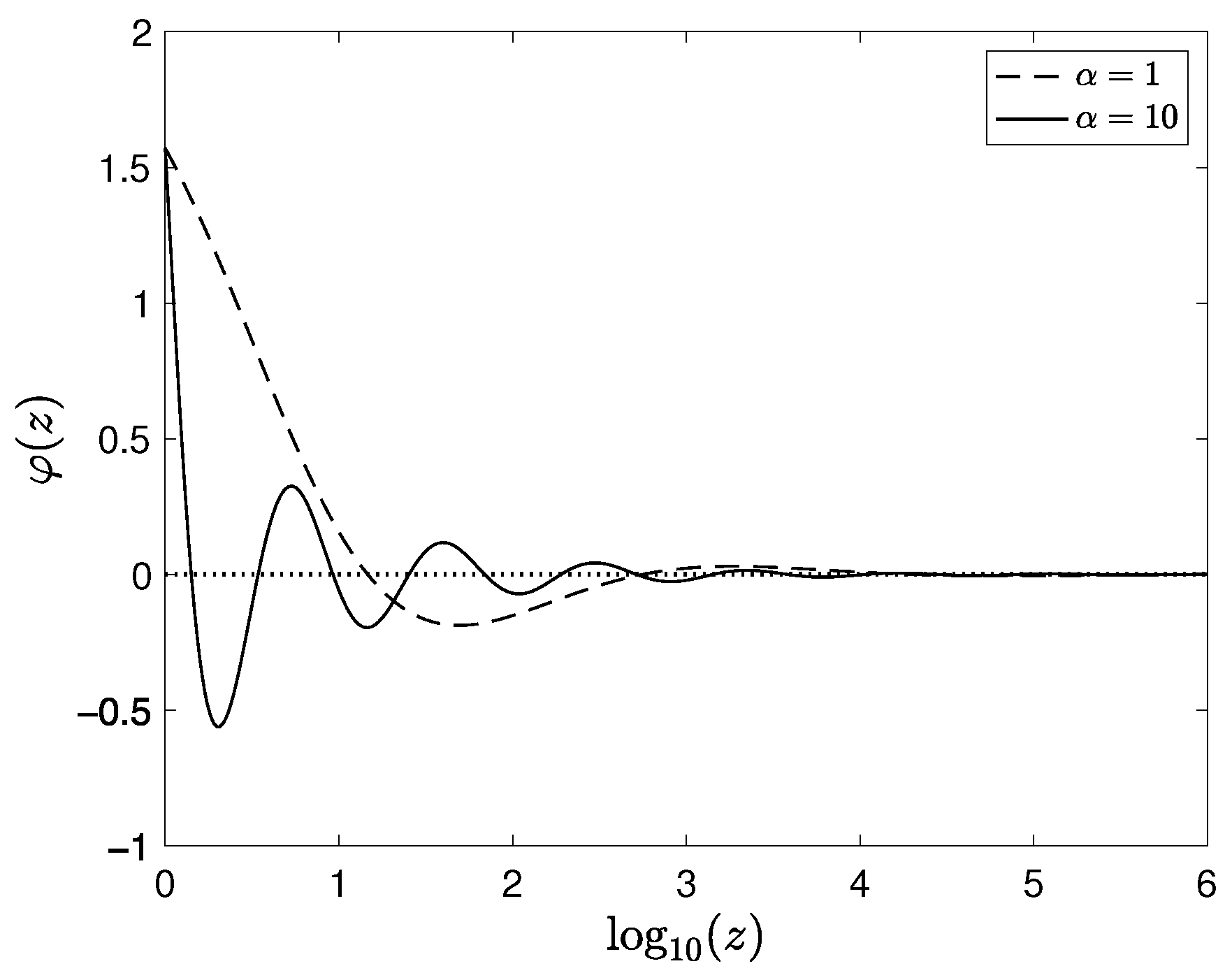
Figure 1 shows illustrative examples of the behavior of bounded solutions for $z>1$. If $0<\phi \left(1\right)<\pi$, then, regardless of the value of $\alpha$, the solutions vanish as $z\to \infty$. The decay is quite slow and, hence, the plots are shown with a logarithmic scale.

In Lemma 4 (Section 2.4), we show, rigorously, that the bounded solutions with $0<\phi \left(1\right)<\pi$ vanish as $z\to \infty$. Therefore, in order to prove the existence of a topologically nontrivial solution, it suffices to find a solution that starts at $0<\phi \left(1\right)<\pi$ and reaches $\phi \left(0\right)=\pi$ when we integrate Equation (3) from $z=1$ to $z=0$.

2.2.3. $\alpha <2$

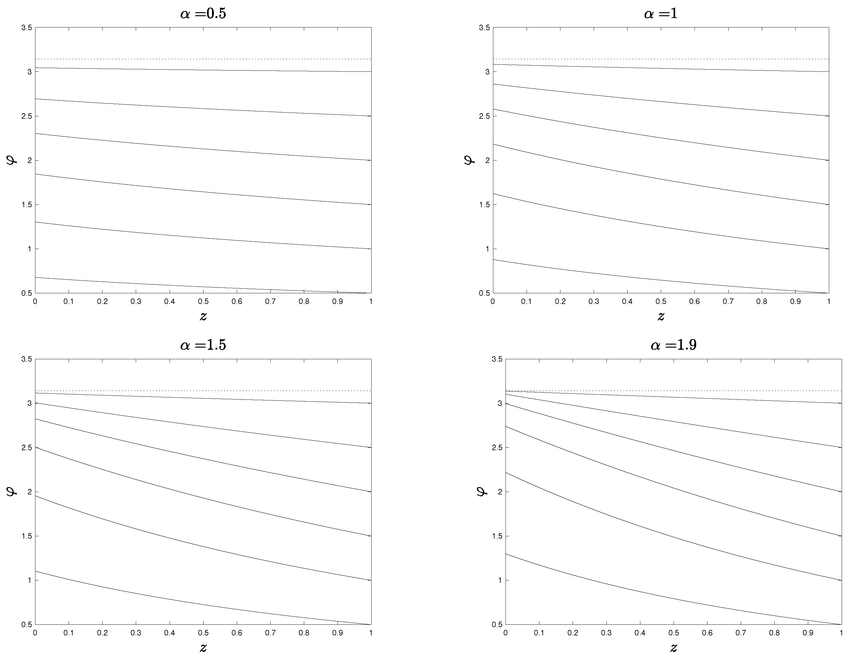
The behavior of solutions for $\alpha <2$ is illustrated in Figure 2. In the graphs, we have started at $z=1^{-}:=1-{10}^{-15},$ and integrated the differential equation back to $z=0$. The noteworthy feature in Figure 2 is that, regardless of what initial value $0<\phi \left(1^{-}\right)<\pi$ is chosen at $z=1^{-}$, $\phi \left(z\right)$ remains strictly between 0 and $\pi$ in the range $0\le z\le 1^{-}$. For $\alpha <2$, a bounded solution with $0<\phi \left(1\right)<\pi$ cannot reach $\phi \left(0\right)=\pi$. Therefore, a solution satisfying the conditions in (5) does not exist for $\alpha <2$.

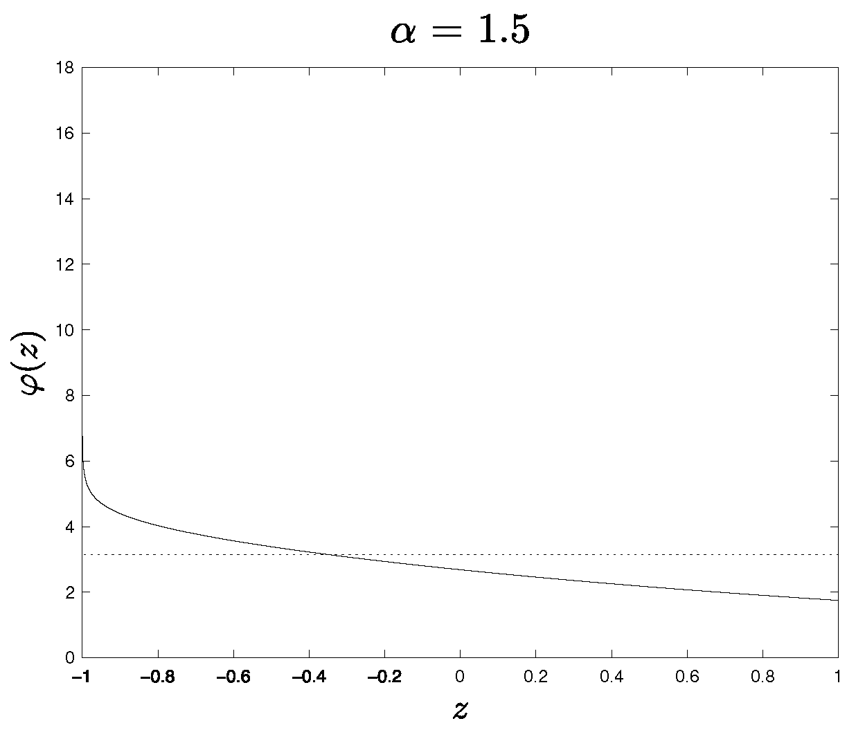
Figure 3 illustrates the behavior of a solution that is bounded in the vicinity of $z=1$ but does not reach $\phi \left(0\right)=\pi$. If  we integrate Equation (3) from $z=1^{-}=1-{10}^{-15}$ past $z=0$ to $z=-1^{+}=-1+{10}^{-14}$, the solution becomes unbounded near $z=-1$ since it does not satisfy the condition analogous to (5), namely ${\phi }^{\prime }(-1)=\alpha /2sin\left(\phi (-1)\right)$, at $z=-1$.

The above discussion represents the content of Theorem 1 (Section 2.5.1), in which we show that, for $\alpha <2$, every bounded solution of Equation (3) is topologically trivial. There are no solitons for $\alpha <2$.

2.2.4. $\alpha >2$

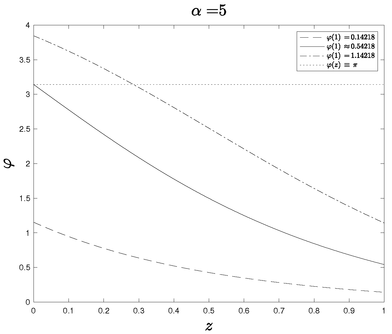
Figure 4 illustrates the behavior of solutions at a sample value of $\alpha >2$, namely $\alpha =5$. For $\phi \left(1^{-}\right)=1.14218,1^{-}=1-{10}^{-15}$, we have $\phi \left(0\right)>\pi$; for $\phi \left(1^{-}\right)=0.14218$, $\phi \left(0\right)<\pi$.

In Lemma A9 (Appendix E), we show that $\phi \left(0\right)$ varies continuously with $\phi \left(1\right)$ for a bounded solution. As we vary $\phi \left(1^{-}\right)$ from 0.14218 to 1.14218, at an intermediate value of $\phi \left(1^{-}\right)$—specifically at $\phi \left(1^{-}\right)\approx 0.54218$—we reach $\phi \left(0\right)=\pi$. Taken together with the asymptotic behavior depicted in Figure 1, Figure 4 shows that topologically nontrivial soliton exists for $\alpha =5$.

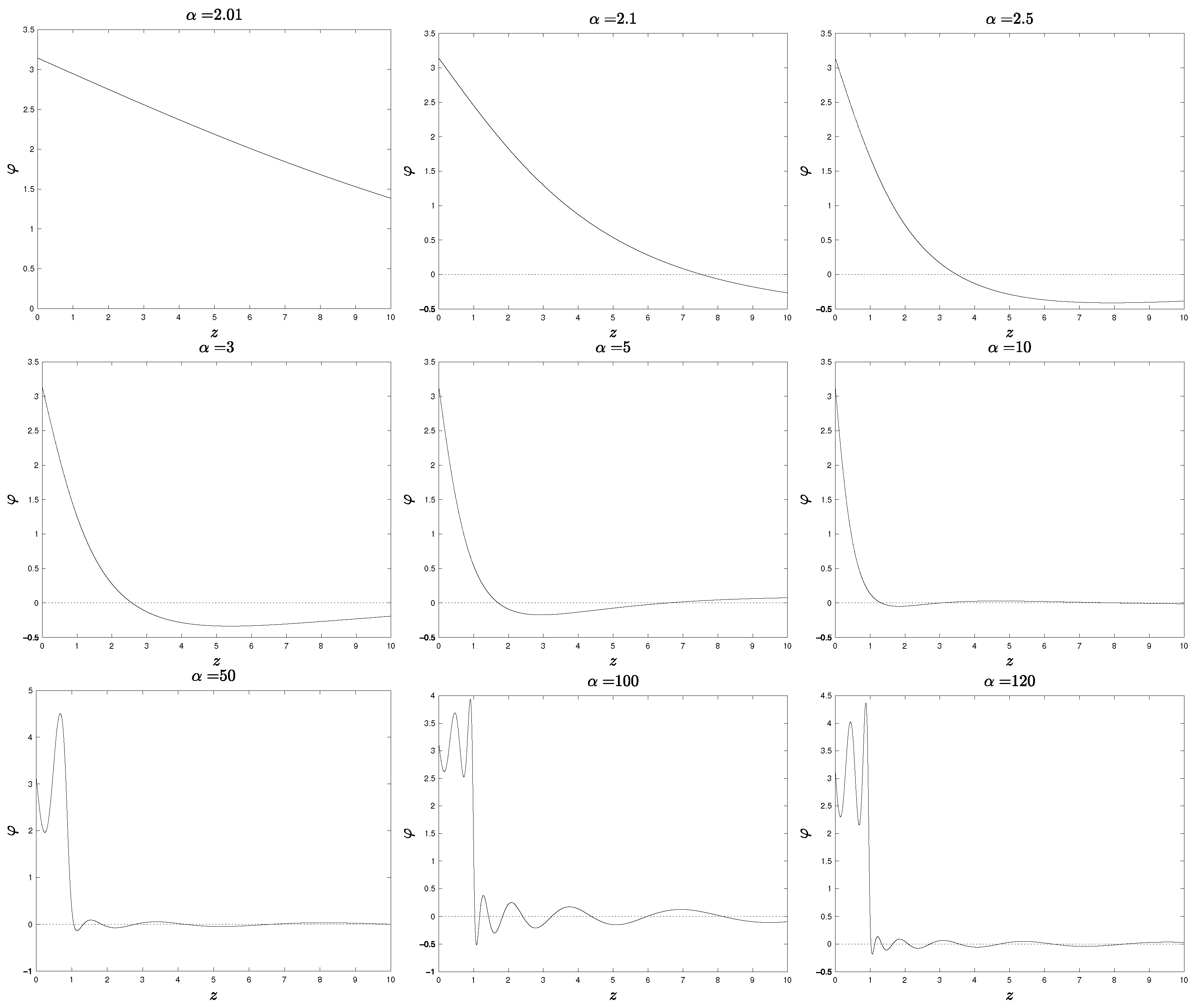
Soliton solutions for some values of $\alpha >2$ are displayed in Figure 5. The range is limited to $0\le z\le 10$ to be able to clearly display the behavior inside the horizon ($0\le z\le 1$). Since the initial condition has to be imposed at $z=1$, to keep the solution bounded, the integration was done separately in two intervals, $0\le z\le 1-{10}^{-15}$ and $1+{10}^{-15}\le z\le 10$, imposing the initial conditions at $1\pm {10}^{-15}$. The  choice of ${10}^{-15}$ is discussed in Section 5.4.

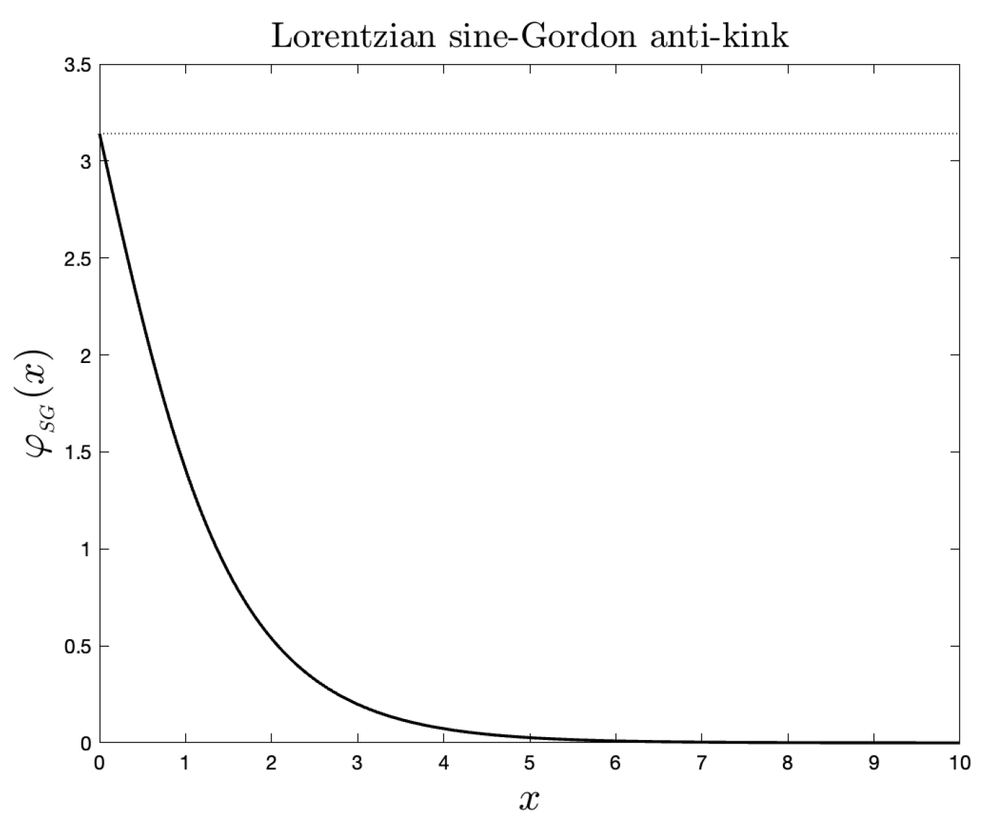
For comparison, in  Figure 6, we have also plotted the Lorentzian sine-Gordon antikink ${\phi }_{SG}\left(x\right)$ that interpolates between the vacuum $\phi =2\pi$ at $x\to -\infty$ and the vacuum $\phi =0$ at $x\to \infty$.

In the following subsections of this section, we state the main results, deferring the proofs to Appendix B, Appendix C, Appendix D and Appendix E. Equation (3) has singularities at $z=\pm 1$, which form the horizon of the region $-1<z<1$. In Section 2.3 we present results that prove the existence of bounded solutions in a neighborhood of the singularity, $z=1$. In Section 2.4, we present results, which show that a solution, $\phi \left(z\right)$, approaches the vacuum that is closest to $\phi \left(1\right)$ as $z\to \infty$. Finally, in Section 2.5, we focus on the region inside the horizon, $-1<z<1$, and present results, which show that solitons exist for $\alpha >2$ and do not exist for $\alpha <2$.

2.3. Bounded Solutions in a Neighborhood of a Singularity

Equation (3) is closely related to the hypergeometric differential equation. We use the known solutions of the hypergeometric differential equations to establish the existence of bounded solutions of Equation (3). In Section 2.3.1 below, we describe the relation between Equation (3) and the hypergeometric equation. In Section 2.3.2, we establish a necessary condition that must be satisfied by a solution at the singularity $z=1$ if it is to be bounded in a neighborhood of the singularity. Finally, in Section 2.3.3, we prove the existence of a 1-parameter family of bounded solutions of Equation (3) in a neighborhood of the singularity $z=1$.

2.3.1. Associated Hypergeometric Equation

The hypergeometric differential equation

$$\begin{array}{c}\hfill x(x-1){\phi }_{xx}+((a+b+1)x-c){\phi }_x+ab\phi =0\end{array}$$

(6)

was first formulated by Euler and was studied extensively by Gauss and Riemann. The relation between Equations (3) and (6) can be seen by transforming from the static coordinate z to the hypergeometric coordinate x, as $x=(1-z)/2$. In hypergeometric coordinate Equation (3) becomes

$$\begin{array}{c}\hfill x(x-1){\phi }_{xx}+(2x-1){\phi }_x+\alpha \phi =f\left(\phi \right)f\left(\phi \right):=\alpha (\phi -sin\left(\phi \right)\end{array}$$

(7)

With a slight abuse of notation we use $\phi$ to denote both the solution $\phi \left(z\right)$ of Equation (3) as well as the solution $\mathrm{\Psi }\left(x\right)=\phi (1-2x)$ of Equation (7).

For $a+b=c=1,ab=\alpha$ in Equation (6), the left-hand side of Equation (6) coincides with the left-hand side of Equation (7). Thus Equation (7) is a nonlinear relative of the hypergeometric differential equation Equation (6). The singularity $z=1$ in Equation (3) corresponds to the singularity $x=0$ in Equation (7).

It is well known that the hypergeometric equation Equation (6) has two linearly independent solutions in a (punctured) neighborhood of $x=0$. For the special values of $a,b,c$ of interest to us, namely $a+b=c=1,ab=\alpha$, the two linearly independent solutions of Equation (6) are denoted ${\phi }_1\left(x\right)$ and ${\phi }_2\left(x\right)$. The first solution, ${\phi }_1\left(x\right)$, is analytic in the neighborhood (−1, 1) and is described in Equation (A4) in Appendix A. The second solution is

$$\begin{array}{c}\hfill {\phi }_2\left(x\right)={\phi }_1\left(x\right)log\left(\right|x\left|\right)+h\left(x\right),x\in (-ϵ,ϵ)\setminus \left\{0\right\}\end{array}$$

(8)

where $h\left(x\right)$ is an analytic function in ($-{\rho }_h,{\rho }_h$) for some $0<{\rho }_h<1$. The  form of ${\phi }_1\left(x\right)$ and the construction of ${\phi }_2\left(x\right)$ are described in Appendix A.

2.3.2. A Necessary Condition for Bounded Solutions

First, we show that, if a solution of Equation (7) is to be bounded at the singularity $x=0$, then it must satisfy the boundary condition described in Lemma 1, stated below.

Lemma 1.

Let ${\phi }_b\left(x\right)$ be a bounded solution of

$$\begin{array}{c}\hfill x(x-1){\phi }_b^{″}+(2x-1){\phi }_b^{\prime }+\alpha sin\left({\phi }_b\right)=0\end{array}$$

(9)

in a neighborhood $(-ϵ,ϵ)$, $ϵ>0$. Then,

$$\begin{array}{c}\hfill \underset{x\to 0}{lim}{\phi }_b^{\prime }\left(x\right)=\alpha sin\left({\phi }_b\left(0\right)\right)\end{array}$$

(10)

The proof of Lemma 1 is presented in Appendix B. Translating Lemma 1 from hypergeometric coordinate to static coordinate, we obtain the following corollary.

Corollary 1.

Let ${\phi }_b\left(z\right)$ be a bounded continuous solution of

$$\begin{array}{c}\hfill (z^2-1){\phi }_b^{″}+2z{\phi }_b^{\prime }+\alpha sin\left({\phi }_b\right)=0\end{array}$$

(11)

in a neighborhood $(1-ϵ,1+ϵ)$, $ϵ>0$. Then,

$$\begin{array}{c}\hfill \underset{z\to 1}{lim}{\phi }_b^{\prime }\left(z\right)=-{\displaystyle \frac{\alpha }{2}}sin\left({\phi }_b\left(1\right)\right)\end{array}$$

(12)

2.3.3. Proof of Existence of Bounded Solutions in a Neighborhood of Singularities

We show that one can obtain a solution of the differential equation Equation (7) by solving a related integral equation, as shown in Lemma 2 below.

Lemma 2.

Let ${\phi }_b\left(x\right)$ be a bounded continuous solution of the integral equation

$$\begin{array}{c}\hfill \begin{array}{c}\phi \left(x\right)={\phi }_2\left(x\right){\int }_0^x\left[{\displaystyle \frac{{\phi }_1\left(y\right)f\left(\phi \left(y\right)\right)}{(y-1)yW\left(y\right)}}\right]dy-{\phi }_1\left(x\right){\int }_0^x\left[{\displaystyle \frac{{\phi }_2\left(y\right)f\left(\phi \left(y\right)\right)}{(y-1)yW\left(y\right)}}\right]dy+\gamma {\phi }_1\left(x\right)\hfill \end{array}\end{array}$$

(13)

in some sufficiently small interval $(-ϵ,ϵ)$, where $0<ϵ<{\rho }_h$. Then, in $(-ϵ,ϵ)$, ${\phi }_b\left(x\right)$ satisfies the differential equation

$$\begin{array}{c}\hfill x(x-1){\phi }_{xx}+(2x-1){\phi }_x+asin\left(\phi \right)=0\end{array}$$

(14)

and the boundary condition described in Lemma 1.

${\phi }_1\left(x\right)$ and ${\phi }_2\left(x\right)$ are described in Equations (A4) and (8). ${\rho }_h$ is defined after Equation (8). $W\left(x\right)$ is the Wronskian of ${\phi }_1$ and ${\phi }_2$. $f\left(\phi \right)=\alpha (\phi -sin(\phi \left)\right)$ and γ is an arbitrary constant.

Thus, to obtain a solution of Equation (7) around $x=0$, it is sufficient to construct a continuous bounded solution of the the integral equation Equation (13) in a neighborhood of $x=0$. The following lemma establishes the existence of a 1-parameter family of such solutions for integral equation  Equation (13).

Lemma 3.

There exists an interval $(-ϵ,ϵ)$, $ϵ>0$ in which the integral equation

$$\begin{array}{c}\hfill \begin{array}{c}\phi \left(x\right)={\phi }_2\left(x\right){\int }_0^x\left[{\displaystyle \frac{{\phi }_1\left(y\right)f\left(\phi \left(y\right)\right)}{(y-1)yW\left(y\right)}}\right]dy-{\phi }_1\left(x\right){\int }_0^x\left[{\displaystyle \frac{{\phi }_2\left(y\right)f\left(\phi \left(y\right)\right)}{(y-1)yW\left(y\right)}}\right]dy+\gamma {\phi }_1\left(x\right)\hfill \end{array}\end{array}$$

(15)

has a 1-parameter family of continuous bounded solutions, ${\phi }_b(x;\gamma )$, labeled by the parameter γ.

Lemmas 2 and 3 are proved in Appendix B. The proofs of Lemmas 2 and 3 rely on technical Lemmas A1–A4, which are stated and proved in Appendix B.

Lemmas 2 and 3 together show that there is a 1-parameter family of bounded solutions, $\phi (x;\gamma )$, of the differential Equation (7) in a neighborhood of the singularity $x=0$. Equivalently, the lemmas also show that there is a 1-parameter family of bounded solutions $\phi (z;\gamma )$ of the differential equation Equation (3) in a neighborhood of the singularity $z=1$.

2.4. Bounded Solutions Outside the Horizon

As shown in Figure 1, bounded solutions approach the vacuum that is closest to $\phi \left(1\right)$ as $z\to \infty$ regardless of the value of $\alpha$. In Lemma 4 below, we prove that bounded solutions, for all $\alpha >0$, behave as shown in Figure 1.

Lemma 4.

Let $\phi \left(z\right)$ be a solution of

$$(z^2-1){\phi }_{zz}+2z{\phi }_z+\alpha sin\left(\phi \right)=0,\alpha >0$$

(16)

satisfying the boundary conditions

$$\begin{array}{c}\hfill {\displaystyle 0<\phi \left(1\right)<\pi ,{\phi }_z\left(1\right)=-\frac{\alpha }{2}sin\left(\phi \left(1\right)\right).}\end{array}$$

(17)

Then, for all $z\ge 1$, we have $-\pi <\phi \left(z\right)<\pi$ and

$$\begin{array}{c}\hfill \underset{z\to \infty }{lim}\phi \left(z\right)=0\end{array}$$

Lemma 4 is proved in Appendix C. Note that, if $\phi$ is a solution of Equation (16), then so are $-\phi$ and $\phi +2n\pi$ for all $n\in \mathbb{Z}$. Therefore, we obtain the following corollary.

Corollary 2.

Let $\phi \left(z\right)$ be a solution of

$$(z^2-1){\phi }_{zz}+2z{\phi }_z+\alpha sin\left(\phi \right)=0,\alpha >0$$

(18)

satisfying the following boundary conditions. For some $n\in \mathbb{Z}$,

$$\begin{array}{c}\hfill {\displaystyle (2n-1)\pi <\phi \left(1\right)<(2n+1)\pi ,{\phi }_z\left(1\right)=-\frac{\alpha }{2}sin\left(\phi \left(1\right)\right).}\end{array}$$

Then, for all $z\ge 1$, we have $(2n-1)\pi <\phi \left(z\right)<(2n+1)\pi$ and

$$\begin{array}{c}\hfill \underset{z\to \infty }{lim}\phi \left(z\right)=2n\pi \end{array}$$

2.5. Bounded Solutions Inside the Horizon

Equation (7) has two length scales—the length scale $m^{-1}$ specified by m, the ‘mass’ parameter of the field, and the length scale $H^{-1}$ of the background spacetime specified by the Hubble parameter H. We say a soliton is ‘large’ if $m^{-1}>H^{-1}/\sqrt{2}$ (that is, if $\alpha :={(m/H)}^2<2$) and ‘small’ if $\alpha >2$.

Inside the horizon, the behavior of bounded solutions depends on whether $\alpha <2$ or $\alpha >2$. We consider the two cases separately, below.

2.5.1. Large Static Solitons Are Forbidden

For $\alpha <2$, solutions that are bounded near $z=1$ with $0<\phi \left(1\right)<\pi$ cannot attain $\phi \left(0\right)=\pi$, as shown by the examples in Figure 2, and blow up at $z=-1$, as shown by the example in Figure 3. The following theorem shows that topologically nontrivial (soliton) bounded solutions do not exist for $\alpha <2$.

Theorem 1.

For $\alpha <2$, every bounded solution of

$$\begin{array}{c}\hfill (z^2-1){\phi }_{zz}+2z{\phi }_z+\alpha sin\left(\phi \right)=0\end{array}$$

(19)

is topologically trivial (i.e., ${lim}_{z\to \infty }\phi \left(z\right)={lim}_{z\to -\infty }\phi \left(z\right))$.

The proof of the theorem is lengthy and is presented in Appendix D. The proof relies on technical Lemmas A5–A8, which are stated and proved in Appendix D. We describe the outline of the proof of Theorem 1, below.

As discussed in Section 2.1, without loss of generality, we can assume that a solitonic field configuration with charge Q satisfies the following conditions:

$$\begin{array}{c}\hfill \underset{z\to -\infty }{lim}\phi \left(z\right)=-2\pi Q,\phi \left(0\right)=-\pi Q,\underset{z\to \infty }{lim}\phi \left(z\right)=0\end{array}$$

Further, given the symmetries of the Lagrangian, we can restrict attention to $z\ge 0$. As Corollary 2 shows, if  we insist that ${lim}_{z\to \infty }\phi \left(z\right)=0$, then we must have $-\pi <\phi \left(1\right)<\pi$.

We prove Theorem 1 by showing that, for  $\alpha <2$ and $-\pi <\phi \left(1\right)<\pi$, every bounded solution satisfies $-\pi <\phi \left(0\right)<\pi$. But a topologically nontrivial soliton, satisfying the above condition, can have integer nonzero charge Q only if $\phi \left(0\right)=\pm \pi Q$. Thus, when $\alpha <2$, topologically nontrivial static solitons cannot exist.

2.5.2. Existence of Small Static Solitons

The behavior of bounded solutions inside the horizon is illustrated for $\alpha =5$ in Figure 4. The  behavior of bounded solutions for all other $\alpha >2$ is qualitatively similar.

In Lemma A9 (Appendix E) we confirm that $\phi \left(0\right)$ is a continuous function of $\phi \left(1\right)$. Using the continuity property, in  Lemmas A10 and A11, we establish that, for  $\alpha >2$, one can find a constant $0<{\gamma }^{\ast }<\pi$ such that, if $\phi \left(1\right)={\gamma }^{\ast }$, then $\phi \left(0\right)=\pi$. Lemmas A10 and A11, together with Corollary 2, prove the following theorem.

Theorem 2.

For every $\alpha >2$, the equation

$$\begin{array}{c}\hfill (z^2-1){\phi }_{zz}+2z{\phi }_z+\alpha sin\left(\phi \right)=0\end{array}$$

has a bounded topologically nontrivial soliton solution.

2.6. Back Reaction

In the above analysis we assumed that the de Sitter background was non-dynamical and we ignored the back reaction of the soliton on the background. In this section, we describe two approaches to incorporating the back reaction of a soliton in order to make the analysis self-consistent. The latter approach, which we adopt, makes the analysis self-consistent and also justifies our assumption that the background de Sitter metric is unaffected by the static soliton for all values of $\alpha$.

It is well known that, due to its symmetries, the Riemann tensor has only one independent component in 1 + 1 dimensional spacetime and is given by

$$\begin{array}{c}\hfill {\displaystyle R_{\alpha \beta \mu \nu }=\frac{R}{2}\left(g_{\alpha \mu }{g}_{\beta \nu }-g_{\alpha \nu }{g}_{\beta \mu }\right)}\end{array}$$

where R is the Ricci scalar and $g_{\mu \nu }$ the metric. As a result, the Einstein tensor $G_{\mu \nu }$ vanishes for every metric in 1 + 1 dimensional spacetime ($R_{\beta \nu }={\displaystyle \frac{1}{2}}R{g}_{\beta \nu }\Rightarrow G_{\beta \nu }=R_{\beta \nu }-{\displaystyle \frac{1}{2}}R{g}_{\beta \nu }=0$). Einstein’s equation

$$\begin{array}{c}\hfill {\displaystyle G_{\mu \nu }+\mathrm{\Lambda }{g}_{\mu \nu }=\kappa T_{\mu \nu },\kappa =\frac{8\pi G_N}{c^4}}\end{array}$$

where $\mathrm{\Lambda }$ is the cosmological constant and $T_{\mu \nu }$ the energy momentum tensor of matter, reduces to

$$\begin{array}{c}\hfill \mathrm{\Lambda }{g}_{\mu \nu }=\kappa T_{\mu \nu }.\end{array}$$

(20)

Since the Einstein tensor vanishes for every metric, one consistent approach in 1 + 1 spacetime would be to take the metric of spacetime to be the solution of Equation (20). If $T_{\mu \nu }$ in Equation (20) comes from the sine-Gordon field, $\varphi$, then $T_{\mu \nu }={\partial }_{\mu }\varphi {\partial }_{\nu }\varphi -g_{\mu \nu }\mathcal{L}$. Therefore,

$$\begin{array}{c}\hfill {\displaystyle g_{\mu \nu }=\left(\frac{\kappa }{\mathrm{\Lambda }}\right)\left[{\partial }_{\mu }\varphi {\partial }_{\nu }\varphi -g_{\mu \nu }\mathcal{L}\right]\mathrm{or}{g}_{\mu \nu }=\frac{\left(\frac{\kappa }{\mathrm{\Lambda }}\right){\partial }_{\mu }\varphi {\partial }_{\nu }\varphi }{1+\left(\frac{\kappa }{\mathrm{\Lambda }}\right)\mathcal{L}}}\end{array}$$

Using the sine-Gordon lagrangian (1), we conclude that the metric $g_{\mu \nu }$ is the solution to

$$\begin{array}{c}\hfill g_{\mu \nu }={\displaystyle \frac{\left(\frac{\kappa }{\mathrm{\Lambda }}\right){\partial }_{\mu }\varphi {\partial }_{\nu }\varphi }{1+\left(\frac{\kappa }{\mathrm{\Lambda }}\right)[\frac{1}{2}{g}^{\alpha \beta }{\partial }_{\alpha }\varphi {\partial }_{\beta }\varphi -(\frac{m^2}{{\beta }^2})(1-cos\left(\beta \varphi \right))]}}.\end{array}$$

(21)

In the action (1), one would use the metric derived as a solution of (21), instead of the de Sitter metric, and attempt to construct a static soliton solution. Even if the nonlinear Equation (21) could be solved, it is not clear, a priori, that, in such an approach the solution of (21) would yield a de Sitter metric or even an approximation to a de Sitter metric (if a soliton interpolates between two vacua, then $T_{\mu \nu }\to 0$ at spatial infinity; therefore, $g_{\mu \nu }\to 0$ asymptotically; such a $g_{\mu \nu }$ would not be a de Sitter metric).

The alternative approach, which we adopt, is to embed sine-Gordon theory that is minimally coupled to gravity, in the so-called Jackiw–Teitelboim (JT) theory of gravity in 1 + 1 spacetime [18,19,20,21]. The JT theory has a term

$$\begin{array}{c}\hfill S_{JT}=\int d^{2}x\sqrt{0in8pt-g}\psi (R-\mathrm{\Lambda })\end{array}$$

that contributes to the bulk action, where $\psi$ is the dilaton field, R, the Ricci scalar and $\mathrm{\Lambda }$, the cosmological constant. There is no kinetic term for $\psi$ in the JT theory. The equation of motion of the dilaton field yields the constraint

$$\begin{array}{c}\hfill R=\mathrm{\Lambda }\end{array}$$

Variation of the total action with respect to the metric yields a dynamical equation for the dilaton field, $\psi$, in which the energy-momentum tensor of the sine-Gordon soliton acts as a source term; the dynamical equation for $\psi$ is obtained by varying the metric, in  both $S_{JT}$ and in the sine-Gordon action, $S_{SG}$, shown in Equation (1), followed by integration by parts to transfer the covariant derivative operators to act on the dilaton field $\psi$. Thus, a matter field, such as the sine-Gordon field, does not impact the metric in JT gravity but, instead, impacts the dynamics of the dilaton field. The metric can be stipulated to be de Sitter and is not impacted by the presence of the sine-Gordon soliton. There is no back reaction of the sine-Gordon soliton on the metric for any value of $\alpha$, and the conclusions of the previous sections, including the threshold $\alpha =2$, remain unchanged.

Taking the metric to be de Sitter in the JT gravity, we can compare the energy in the static soliton inside the horizon with the energy resident in the cosmological constant inside the horizon. A straightforward derivation of the Riemann tensor, starting with the de Sitter metric, shows that the Riemann tensor in de Sitter spacetime is

$$\begin{array}{c}\hfill R_{\alpha \beta \mu \nu }=H^2(g_{\alpha \mu }{g}_{\beta \nu }-g_{\alpha \nu }{g}_{\beta \mu }).\end{array}$$

Hence, we conclude that $\mathrm{\Lambda }=2H^2$.

Starting with the action (1), and using the previous convention $\phi \left(z\right):=\beta \psi (z/H)$, where $\varphi (t,\chi ):=\psi \left(u\right),u=e^{Ht}\chi$, a straightforward calculation yields the energy density

$$\begin{array}{c}\hfill T^{00}={\displaystyle \frac{H^2}{{\beta }^2}}\left\{{\displaystyle \frac{1}{2}}(z^2+1){\phi }_z^2+\alpha (1-cos\left(\phi \right))\right\}={\displaystyle \frac{\mathrm{\Lambda }}{2{\beta }^2}}\left\{{\displaystyle \frac{1}{2}}(z^2+1){\phi }_z^2+\alpha (1-cos\left(\phi \right))\right\}\end{array}$$

As is well known [22], the weak coupling regime corresponds to ${\beta }^2<8\pi$. So, we set ${\beta }^2={\beta }_0^2:=8\pi -{10}^{-6}$. Focusing on the regime $\alpha \sim 2$, we take $\alpha ={\alpha }_0:=2.0001$. Then, the ratio of the soliton’s energy within the horizon, denoted $E_S$, to the energy due to the cosmological constant within the horizon, denoted $E_{\mathrm{\Lambda }}$, in units where $8\pi G=c=1$, is obtained numerically as

$$\begin{array}{c}\hfill {\displaystyle \frac{E_S}{E_{\mathrm{\Lambda }}}=\frac{{\displaystyle {\int }_{-1}^1\frac{\mathrm{\Lambda }}{2{\beta }_0^2}\left\{\frac{1}{2}(z^2+1){\phi }_z^2+{\alpha }_0(1-cos\left(\phi \right))\right\}dz}}{2\mathrm{\Lambda }}\approx 0.0796}\end{array}$$

(22)

The integral in (22) was evaluated as a Riemann sum with ∼$2\times {10}^9$ mesh points in the range $(-1,1)$ using MATLAB R2024b. The computation was done using double precision. Equation (3) was integrated using ode45, a built-in function in MATLAB R2024b. The computation was started at $z=1-{10}^{-9}$ and integrated backwards to $z=-1+{10}^{-9}$; the displacement of ${10}^{-9}$ was determined by memory constraints on the size of the grid. The integrity of the computation was verified by confirming that ${\phi }_z(1-{10}^{-9})={\phi }_z(-1+{10}^{-9})$. Within the horizon, the energy in the soliton field is ∼8% of the energy due to the cosmological constant for the above choice of parameter values in the weak coupling regime.

3. Heuristic Estimates Based on Tensile and Tidal Forces

In this section, we present heuristic arguments based on the interplay of tensile force and tidal force. On the one hand, the tensile force of a soliton resists inflationary stretching of the soliton and acts to preserve a soliton as a compact field configuration. On the other hand, the tidal force of the inflationary background tends to stretch the soliton. If a soliton is to be static, that is, if  its physical dimensions are to buck inflationary stretching, then its internal tensile force must be strong enough to counteract the tidal stretching of the soliton by the background. The arguments we present are crude. They have only a qualitative heuristic value.

In Section 3.1, we use a heuristic argument to obtain an estimate of the tensile force in a Lorentzian sine-Gordon soliton and, using the estimate, a threshold for existence of a static sine-Gordon soliton in a de Sitter background; the estimate we obtain with the crude heuristic argument agrees with the exact estimate $\alpha =2$ to  within an $O\left(1\right)$ factor.

In Section 3.2, we use a similar heuristic argument to obtain an estimate of the tensile force in a Lorentzian $SO\left(3\right)$ 't Hooft–Polyakov monopole and, using the estimate, a threshold for existence of static $SO\left(3\right)$ 't Hooft–Polyakov monopole in a de Sitter background. The existence of the threshold, suggested by our heuristic argument, remains to be confirmed by an analytical argument. Guided by the heuristic argument, we propose a conjecture that there is an $O\left(1\right)$ threshold for the existence of a static $SO\left(3\right)$ 't Hooft–Polyakov monopole in non-dynamical de Sitter background.

3.1. Sine-Gordon Solitons

In spacetime with nonzero Riemann tensor the separation between two neighboring, initially parallel, geodesics accelerates as one moves along the fiducial geodesic. Since a soliton is an extended object two neighboring points in a soliton move along different geodesics. In de Sitter spacetime the separation between two neighboring points grows with time; in other words, the de Sitter background pulls the points apart. If the soliton is to remain a compact static object, the internal tensile forces of the soliton must be strong enough to resist the tidal force of the background spacetime that seeks to tear the soliton apart.

A rigorous study of the interplay between the internal tensile force of a soliton and the tidal force of the background requires analysis of the soliton configuration in the curved background. We consider a simpler problem. We estimate the tensile force in a sine-Gordon soliton in 1 + 1 Lorentzian spacetime and compare it with the tidal force operative in de Sitter spacetime. We show that even the rather simple analysis is able to reproduce the rigorously derived threshold to within an $O\left(1\right)$ factor.

In a Lorentzian background the sine-Gordon Lagrangian is

$$\begin{array}{c}\hfill \mathcal{L}={\displaystyle \frac{1}{2}}{\partial }_{\mu }\phi {\partial }^{\mu }\phi -U\left(\phi \right),U\left(\phi \right):=m^2\left(1-cos\left(\phi \right)\right)\end{array}$$

(23)

(The Lorentzian sine-Gordon field $\phi$ has been redefined to absorb the coupling constant $\beta$; the resulting overall multiplicative factor, ${\beta }^{-2}$, is irrelevant to our argument; see Equation (30)). Time-independent solutions of the Euler–Lagrange equation satisfy

$$\begin{array}{c}\hfill {\phi }_{xx}\left(x\right)=U^{\prime }\left(\phi \right)\end{array}$$

(24)

As Coleman observed, if we interpret x as time and $\phi$ as the position of a particle, then Equation (24) describes the behavior of a particle of unit mass moving in potential $-U\left(\phi \right)$. A soliton solution that interpolates between two adjacent minima of $U\left(\phi \right)$ corresponds to the trajectory of the particle moving, from infinite past to infinite future, between two adjacent maxima of $-U\left(\phi \right)$. Since the energy of the particle is conserved, and, assuming the potential energy as well as the kinetic energy of the particle at the local maximum of $-U\left(\phi \right)$ is zero, we have

$$\begin{array}{c}\hfill {\displaystyle \frac{1}{2}}{\left({\phi }^{\prime }\left(x\right)\right)}^2=U\left(\phi \right)\end{array}$$

(25)

One can verify that the time-independent topologically nontrivial soliton solution of the sine-Gordon theory, $\tilde{\phi }\left(x\right)$, given by

$$\begin{array}{c}\hfill \tilde{\phi }\left(x\right)=4{tan}^{-1}\left(e^{mx}\right)\end{array}$$

(26)

satisfies Equation (25). From Equation (25) we see that the energy density of the soliton $\tilde{\phi }$ is given by

$$\begin{array}{c}\hfill {\displaystyle \mathcal{E}\left(x\right)=\frac{1}{2}{(\tilde{\phi }\prime \left(x\right))}^2+U\left(\tilde{\phi }\left(x\right)\right)=2U\left(\tilde{\phi }\left(x\right)\right)=16m^2\left[\frac{e^{2mx}}{{(1+e^{2mx})}^2}\right]}\end{array}$$

Thus, most of the energy of the sine-Gordon soliton is contained within a distance of $l\sim \xi m^{-1}$ from the center, where $\xi \sim O\left(1\right)$. We define a system S to be the soliton configuration within a fiducial box $[-l,l]$ and the energy contained in the system S as

$$\begin{array}{c}\hfill {\displaystyle E\left(l\right)==2{\int }_0^l\mathcal{E}\left(x\right)dx=8m\left[\frac{e^{2ml}-1}{e^{2ml}+1}\right];E(\infty )-E\left(l\right)=\frac{16m}{e^{2ml}+1}}\end{array}$$

(27)

Consider stretching the soliton as ${\tilde{\phi }}_{\lambda }\left(x\right)=\tilde{\phi }(x/\lambda ),\lambda \ge 1$, where ${\tilde{\phi }}_{\lambda }\left(x\right)$ represents the stretched configuration. As a result of the stretching, the fiducial segment of the soliton in the interval $[-l,l]$ stretches to span $[-\lambda l,\lambda l]$, and the energy in the stretched segment, denoted $E_{\lambda }\left(\lambda l\right)$, is given by

$$\begin{array}{c}\hfill E_{\lambda }\left(\lambda l\right)=2{\int }_0^{\lambda l}\left[{\displaystyle \frac{1}{2}}{\left({\tilde{\phi }}_{\lambda }^{\prime }\left(x\right)\right)}^2+U\left({\tilde{\phi }}_{\lambda }\left(x\right)\right)\right]dx=\left({\displaystyle \frac{1}{2}}\right)\left[\lambda +(1/\lambda )\right]E\left(l\right)\end{array}$$

The increase in the internal energy in the fiducial system as a result of the stretching is

$$\begin{array}{c}\hfill \Delta E_{\lambda }=E_{\lambda }\left(\lambda l\right)-E\left(l\right)={\displaystyle \frac{1}{2}}\left(\lambda +{\displaystyle \frac{1}{\lambda }}-2\right)E\left(l\right)\end{array}$$

(28)

Clearly $E_{\lambda }\left(\lambda l\right)$ is minimized at $\lambda =1$, and the increase in the internal energy in the system S can be interpreted as the work done on the system against its internal tensile force, which resists stretching. We define $F\left(\lambda \right)$ as the centripetal tensile force acting at the boundary of the stretched fiducial segment that has been stretched by a factor $\lambda$. Denoting the change in the size of the system as $q:=2(\lambda l-l)$, we have

$$\begin{array}{c}\hfill \Delta E_{\lambda }=2{\int }_1^{\lambda }F\left(v\right)ldv\end{array}$$

from which we obtain

$$\begin{array}{c}\hfill {\displaystyle F\left(\lambda \right)=\left(\frac{1}{2l}\right)\frac{d}{d\lambda }\Delta E_{\lambda }=\left(\frac{1}{4l}\right)E\left(l\right)\left({\displaystyle 1-\frac{1}{{\lambda }^2}}\right)}\end{array}$$

(29)

$F\left(\lambda \right)$ is the centripetal force that the system S exerts at $x=\lambda l$ on its complement, which is the segment of the stretched soliton beyond $\lambda l$. The mass of the complement, denoted $m_c$ in units in which the velocity of light in vacuum, $c=1$, is

$$\begin{array}{c}\hfill m_C:={\displaystyle \frac{1}{2}}\left(E_{\lambda }(\infty )-E_l\left(\lambda l\right)\right)={\displaystyle \frac{1}{2}}\left(\lambda +{\displaystyle \frac{1}{\lambda }}\right)(E(\infty )-E\left(l\right))\end{array}$$

Assuming that the complement of the stretched system behaves like a rigid body, the centripetal acceleration at $x=\lambda l$ that arises when the external stretching force is turned off is

$$\begin{array}{c}\hfill {\displaystyle a_{\lambda }=\frac{F\left(\lambda \right)}{m_C}=\frac{e^{2ml}-1}{4l}\left[\frac{{\lambda }^2-1}{\lambda ({\lambda }^2+1)}\right]}\end{array}$$

(30)

(The overall factor ${\beta }^{-2}$ that arises from the redefinition of the field (see the remark after Equation (23)) appears in both $F\left(\lambda \right)$ and $m_C$, and is hence irrelevant to the calculation of $a_{\lambda }$ in Equation (30), as we remarked earlier.)

The centrifugal tidal acceleration of the displacement ${\chi }^{\alpha }$ is given by [23]

$$\begin{array}{c}\hfill a_t^{\alpha }={\nabla }_u{\nabla }_u{\chi }^{\alpha }=-R_{\beta \mu \nu }^{\alpha }{u}^{\beta }{u}^{\nu }{\chi }^{\mu }\end{array}$$

where $u^{\beta }$ and $u^{\nu }$ are the tangents to the two geodesics and ${\chi }^{\mu }$ the displacement between the two geodesics. It should be noted that the expression for tidal acceleration holds only for small displacement. We show below that the small-displacement assumption is satisfied in our argument; see the discussion preceding and following Equation (35). We take $u^{\beta }=u^{\nu }=(1,0)$. Therefore, the components of the Riemann tensor of interest to us are $R_{0\mu 0}^{\alpha }$. Calculation of the Riemann tensor shows the only nonzero component of $R_{0\mu 0}^{\alpha }$ is $R_{010}^1=-H^2$. Taking ${\chi }^{\alpha }=(0,\lambda l)$, the tidal acceleration is

$$\begin{array}{c}\hfill a_t=H^2\lambda l\end{array}$$

(31)

Consider stretching the sine-Gordon soliton using external force by a factor $\lambda$ in Lorentzian spacetime, as  described above. As a result of the stretching, centripetal tensile forces arise in the soliton, as described in Equation (29). At $t=0$ we turn off the external stretching force and simultaneously turn on the expansion of the background de Sitter spacetime with Hubble parameter H. The de Sitter background induces a centrifugal tidal acceleration in the soliton. The question we are interested in is: For what value of λ are the centripetal tensile acceleration of the soliton and the centrifugal tidal acceleration balanced at the boundary of the stretched fiducial system?

We take the size of the fiducial system S to be $l=m^{-1}$, the characteristic size of the sine-Gordon soliton. Equating the tensile and tidal accelerations at $l=m^{-1}$ using Equations (30) and (31) and setting $\alpha ={(m/H)}^2$, we obtain

$$\begin{array}{c}\hfill {\displaystyle \frac{{\lambda }^2-1}{{\lambda }^2({\lambda }^2+1)}=q,q:=\left[\frac{4}{e^2-1}\right]\frac{1}{\alpha }\approx \frac{0.6261}{\alpha }}\end{array}$$

Setting $w={\lambda }^2$, we obtain the equation

$$\begin{array}{c}\hfill q{w}^2+(q-1)w+1=0\end{array}$$

(32)

We need at least one of the solutions of the above quadratic equation to be positive, which can happen only if $q<1$, that is, $\alpha \gtrsim 0.6261$. In addition, since $w={\lambda }^2$ must be real, we must have ${(q-1)}^2-4q\ge 0$, or, in terms of $\alpha \approx 0.6261/q$, we must have

$$\begin{array}{c}\hfill (\alpha -0.1074)(\alpha -3.6490)\ge 0\end{array}$$

(33)

The inequality (33) is satisfied if $\alpha \lesssim 0.1074$ or $\alpha \gtrsim 3.6490$. Since positivity of w requires $\alpha \gtrsim 0.6261$, we conclude that a real $\lambda$ exists only if

$$\begin{array}{c}\hfill \alpha \gtrsim 3.6490\end{array}$$

(34)

For $\alpha \lesssim 3.6490$, $\lambda$ would be complex, which means that tensile and tidal accelerations cannot be at equilibrium at the boundary of the fiducial system S at any real $\lambda$; in other words, the system cannot be a static configuration. It is worth comparing the inequality (34) with the result of the exact analysis in Section 2, which showed that static soliton exists only if $\alpha >2$.

In using the expression for tidal acceleration, we made the assumption that the displacement $\lambda l$ was ‘small’. That is, in terms of the characteristic length scale of the background, we assumed $\lambda l/H^{-1}\lesssim 1$. For $l\sim m^{-1}$, the assumption we made was

$$\begin{array}{c}\hfill \lambda \lesssim \sqrt{\alpha }.\end{array}$$

(35)

As verified below, the assumption is always satisfied by the smaller root of Equation (32), denoted ${\lambda }_1$. At ${\lambda }_1$, the inequality (35) can be written as

$$\begin{array}{c}\hfill 1-q-2q\alpha <\sqrt{{(1-q)}^2-4q}\end{array}$$

(36)

Since $2q\alpha \approx 1.2521>1$ and $q>0$, the  left-hand side of (36) is negative and inequality (36) is always satisfied for $\alpha >$ 3.6490.

The above analysis is crude since it estimates the tensile force of the soliton in Lorentzian and not de Sitter spacetime.

3.2. 't Hooft–Polyakov Monopole

In this section we compare a heuristic estimate of the tensile force within the Lorentzian 't Hooft–Polyakov monopole, in the Prasad–Sommerfeld limit, and the tidal force the monopole experiences in de Sitter spacetime to obtain a heuristic threshold for the existence of static 't Hooft–Polyakov monopole in de Sitter spacetime. 't Hooft–Polyakov monopoles are solitons of a Yang–Mills gauge theory in which the gauge fields couple to a triplet of Higgs scalars. The Lagrangian is

$$\begin{array}{c}\hfill \mathcal{L}=-{\displaystyle \frac{1}{4}}{G}_{\mu \nu }^a{\left(G^{\mu \nu }\right)}^a+{\displaystyle \frac{1}{2}}{D}_{\mu }{\phi }^a{D}^{\mu }{\phi }^a-{\displaystyle \frac{\xi }{4}}{({\phi }^a{\phi }^a-F^2)}^2,a=1,2,3\end{array}$$

(37)

where F is the minimum of the Higgs potential, and 

$$\begin{array}{c}\hfill {\left(D_{\mu }\phi \right)}^a={\partial }_{\mu }{\phi }^a+g{ϵ}^{abc}{A}_{\mu }^b{\phi }^c,G_{\mu \nu }^a={\partial }_{\mu }{A}_{\nu }^a-{\partial }_{\nu }{A}_{\mu }^a+g{ϵ}^{abc}{A}_{\mu }^b{A}_{\nu }^c,a,b,c=1,2,3\end{array}$$

The equations of motion are

$$\begin{array}{c}\hfill {\left(D_{\mu }{D}^{\mu }\phi \right)}^a=-\xi ({\phi }^2-F^2){\phi }^a,D_{\mu }{\left(G^{\mu \nu }\right)}^a=g{ϵ}^{abc}{\left(D^{\nu }\phi \right)}^b{\phi }^c\end{array}$$

If we choose the temporal gauge $A_0^a=0$ and consider a time-independent solution, then the energy is given by

$$\begin{array}{c}\hfill E=\int d^{3}x\left\{{\displaystyle \frac{1}{4}{\left(G_{ij}\right)}^a{\left(G_{ij}\right)}^a+\frac{1}{2}{\left(D_i\phi \right)}^a{\left(D_i\phi \right)}^a+\frac{\xi }{4}{({\phi }^2-F^2)}^2}\right\}\end{array}$$

where the sum over repeated indices is implied; that is,

$$\begin{array}{c}\hfill {\left(G_{ij}\right)}^a{\left(G_{ij}\right)}^a=\sum _{i,j,a=1}^3{\left(G_{ij}^a\right)}^2,{\left(D_i\phi \right)}^a{\left(D_i\phi \right)}^a=\sum _{i,a=1}^3{\left(D_i{\phi }^a\right)}^2.\end{array}$$

In the Prasad–Sommerfeld limit [24], in which the Higgs self-coupling vanishes, the equations of motion are

$$\begin{array}{c}\hfill {\left(D_i{D}^i\phi \right)}^a=0,D_i{\left(G^{ij}\right)}^a=g{ϵ}^{abc}{\left(D^j\phi \right)}^b{\phi }^c\end{array}$$

(38)

and the energy is

$$\begin{array}{c}\hfill E=\int d^{3}x\mathcal{H},\mathcal{H}=\left\{{\displaystyle \frac{1}{4}}{\left(G_{ij}\right)}^a{\left(G_{ij}\right)}^a+{\displaystyle \frac{1}{2}}{\left(D_i\phi \right)}^a{\left(D_i\phi \right)}^a\right\}\end{array}$$

(39)

Prasad and Sommerfeld showed that the equations of motion Equation (38) are satisfied by

$$\begin{array}{c}\hfill \begin{array}{c}{\phi }^a=x^{a}K\left(r\right),K\left(r\right)=\left({\displaystyle \frac{1}{g{r}^2}}\right)\left[m_{V}rcoth\left(m_{V}r\right)-1\right]\hfill \\ \hfill \\ A_i^a={ϵ}_{aij}{x}^{j}W\left(r\right),W\left(r\right)=\left({\displaystyle \frac{1}{g{r}^2}}\right)\left[1-m_{V}r/sinh\left(m_{V}r\right)\right]\hfill \end{array},m_V=gF;\end{array}$$

(40)

Further, the solution shown in Equation (40) satisfies the Bogomolny equation

$$\begin{array}{c}\hfill {\displaystyle \frac{1}{2}}{ϵ}^{ijk}{G}_{ij}^a=-{\left(D^k\phi \right)}^a\end{array}$$

from which we obtain the equipartition of energy density between the Higgs and gauge fields

$$\begin{array}{c}\hfill {\displaystyle \frac{1}{2}}{\left(D_i\phi \right)}^a{\left(D_i\phi \right)}^a={\displaystyle \frac{1}{4}}{G}_{ij}^a{\left(G_{ij}\right)}^a\end{array}$$

(41)

Using the notation of Equations (39) and (40) we see that the energy density of the soliton is spherically symmetric

$$\begin{array}{c}\hfill \mathcal{H}\left(r\right)={\mathcal{H}}_A\left(r\right)+{\mathcal{H}}_{\phi }\left(r\right),{\mathcal{H}}_{\phi }\left(r\right)={\displaystyle \frac{1}{2}}{\left(D_i\phi \right)}^a{\left(D_i\phi \right)}^a,{\mathcal{H}}_A\left(r\right)={\displaystyle \frac{1}{4}}{G}_{ij}^a{\left(G_{ij}\right)}^a\end{array}$$

The characteristic length scale of the soliton is $\rho \sim m_V^{-1}$. We define the fiducial system, S, as the Higgs and gauge field configurations in the static soliton within a sphere of radius $\rho \sim m_V^{-1}$ centered at the origin. The energy in the system and its complement are

$$\begin{array}{c}\hfill E\left(\rho \right)=4\pi {\int }_0^{\rho }{r}^2\mathcal{H}\left(r\right)dr,E^{\left(c\right)}\left(\rho \right)=4\pi {\int }_{\rho }^{\infty }{r}^2\mathcal{H}\left(r\right)dr,\end{array}$$

(42)

Following the argument for the sine-Gordon soliton, we stretch the soliton with a dilatation $\overrightarrow{y}=\lambda \overrightarrow{x},\lambda >1$. The Higgs and gauge fields in the new coordinate system are

$$\begin{array}{c}\hfill {\displaystyle \tilde{\phi }\left(\overrightarrow{y}\right)=\phi (\overrightarrow{y}/\lambda ),{\tilde{A}}_i^a\left(\overrightarrow{y}\right)=\frac{1}{\lambda }{A}_i^a(\overrightarrow{y}/\lambda )}\end{array}$$

The energy densities of the Higgs and gauge fields in the stretched system are denoted ${\tilde{\mathcal{H}}}_{\tilde{\phi }}\left(r\right)$ and ${\tilde{\mathcal{H}}}_{\tilde{A}}\left(r\right)$. The energy in the stretched system is

$$\begin{array}{c}\hfill \tilde{E}\left(\lambda \rho \right)=4\pi {\int }_0^{\lambda \rho }{r}^2\left[{\tilde{\mathcal{H}}}_{\tilde{A}}\left(r\right)+{\tilde{\mathcal{H}}}_{\tilde{\phi }}\left(r\right)\right]dr=4\pi {\lambda }^3{\int }_0^{\rho }{s}^2\left[{\left({\displaystyle \frac{1}{\lambda }}\right)}^4{\mathcal{H}}_A\left(s\right)+{\left({\displaystyle \frac{1}{\lambda }}\right)}^2{\mathcal{H}}_{\phi }\left(s\right)\right]ds\end{array}$$

Using the equipartition of energies shown in Equation (41) we obtain

$$\begin{array}{c}\hfill \tilde{E}\left(\lambda \rho \right)={\displaystyle \frac{1}{2}}\left(\lambda +{\displaystyle \frac{1}{\lambda }}\right)E\left(\rho \right)\end{array}$$

The increase in the internal energy of the system, as a result of stretching, is the work done against the negative pressure $P\left(\lambda \right)$ in the system and is

$$\begin{array}{c}\hfill \Delta E=\tilde{E}\left(\lambda \rho \right)-E\left(\rho \right)={\displaystyle \frac{1}{2}}\left(\lambda +{\displaystyle \frac{1}{\lambda }}-2\right)E\left(\rho \right)={\int }_1^{\lambda }P\left({\lambda }^{\prime }\right)dV={\int }_1^{\lambda }f\left({\lambda }^{\prime }\right)\rho d\left({\lambda }^{\prime }\right)\end{array}$$

where $f\left({\lambda }^{\prime }\right)$, the total centripetal restoring force arising at the boundary of the system stretched by a factor ${\lambda }^{\prime }$, is given by

$$\begin{array}{c}\hfill {\displaystyle f\left(\lambda \right)=\frac{1}{\rho }\frac{d\Delta E}{d\lambda }=\frac{1}{2\rho }\left(1-\frac{1}{{\lambda }^2}\right)E\left(\rho \right)}\end{array}$$

(43)

We assume that the centripetal force at the boundary of the stretched system acts on the complement of the stretched system, which we assume behaves as a rigid body of mass $\overline{m}$ given by

$$\begin{array}{c}\hfill \overline{m}=4\pi {\int }_{\lambda \rho }^{\infty }{r}^2\left[{\tilde{\mathcal{H}}}_{\tilde{\phi }}\left(r\right)+{\tilde{\mathcal{H}}}_{\tilde{A}}\left(r\right)\right]dr={\displaystyle \frac{1}{2}}\left({\displaystyle \lambda +\frac{1}{\lambda }}\right)E^{\left(c\right)}\left(\rho \right)\end{array}$$

where $E^{\left(c\right)}\left(\rho \right)$ is defined in Equation (42). The magnitude of the centripetal tensile acceleration, as a function of scale factor $\lambda$, is then

$$\begin{array}{c}\hfill {\displaystyle a_{\lambda }=\frac{\left({\lambda }^2-1\right)}{\lambda \rho \left({\lambda }^2+1\right)}\frac{E\left(\rho \right)}{E^{\left(c\right)}\left(\rho \right)}}\end{array}$$

(44)

To determine the tidal force in 3 + 1 de Sitter, again we take the tangents of the fiducial and a nearby spatially separated geodesic to be $u=(1,0,0,0)$. The spatial separation between the geodesics is taken to be $\chi =(0,\overrightarrow{\chi })$. Then the relevant components of the Riemann tensor are $R_{0j0}^i$. Straightforward calculation yields

$$\begin{array}{c}\hfill R_{0j0}^i=-{\delta }_j^i{H}^2\end{array}$$

where H is the Hubble constant. Then the magnitude of the centrifugal tidal acceleration at the boundary of the stretched system, that is, at a distance $\lambda \rho =\lambda /m_V$ from the origin, is

$$\begin{array}{c}\hfill a_t=H^2\lambda \rho =H^2\left({\displaystyle \frac{\lambda }{m_V}}\right)\end{array}$$

(45)

The tensile and tidal accelerations are balanced at the boundary of the stretched system if, at $r=\lambda /m_V$, we have, using Equations (44) and (45),

$$\begin{array}{c}\hfill {\displaystyle \frac{({\lambda }^2-1)}{{\lambda }^2({\lambda }^2+1)}=\frac{1}{\kappa {\alpha }^{\left(tP\right)}}}\end{array}$$

(46)

where ${\alpha }^{\left(tP\right)}:={(m_V/H)}^2$, and $\kappa :=E\left(m_V^{-1}\right)/E^{\left(c\right)}\left(m_V^{-1}\right)$. Setting $w:={\lambda }^2$, the above equation becomes

$$\begin{array}{c}\hfill w^2+(1-\kappa {\alpha }^{\left(tP\right)})w+\kappa {\alpha }^{\left(tP\right)}=0\end{array}$$

(47)

Using Equations (40) and (41) it can be verified that

$$\begin{array}{c}\hfill \mathcal{H}\left(r\right)={(r{K}^{\prime }\left(r\right)+K\left(r\right))}^2+2K{\left(r\right)}^2{(1-g{r}^{2}W\left(r\right))}^2\end{array}$$

(48)

Since $\mathcal{H}\left(r\right)\ge 0$, from (42) and the definition of $\kappa$, it follows that $\kappa \ge 0$. Using (48) and (42), $\kappa$ can be obtained by numerical integration to be $\kappa \approx 1.4820$. Recalling that ${\alpha }^{\left(tP\right)}\ge 0$, consistency of (46) requires that ${\lambda }^2\ge 1$. From (46), it then follows that $\kappa {\alpha }^{\left(tP\right)}\ge 1$ or

$$\begin{array}{c}\hfill {\displaystyle {\alpha }^{\left(tP\right)}\ge \frac{1}{\kappa }\approx 0.6748}\end{array}$$

(49)

Further, for $w={\lambda }^2$ to be real, we must have

$$\begin{array}{c}\hfill {(1-\kappa {\alpha }^{\left(tP\right)})}^2-4\kappa {\alpha }^{\left(tP\right)}=(\kappa {\alpha }^{\left(tP\right)}-(3+2\sqrt{2}))(\kappa {\alpha }^{\left(tP\right)}-(3-2\sqrt{2}))\ge 0\end{array}$$

or

$$\begin{array}{c}\hfill {\alpha }^{\left(tP\right)}\le 0.1158,or{\alpha }^{\left(tP\right)}\ge 3.9328\end{array}$$

(50)

From (49) and (50) we conclude that, if ${\alpha }^{\left(tP\right)}={(m_V/H)}^2<3.9328$, then there is no (real) scale factor at which the tidal and tensile forces can reach equilibrium at $r=\lambda /m_V$.

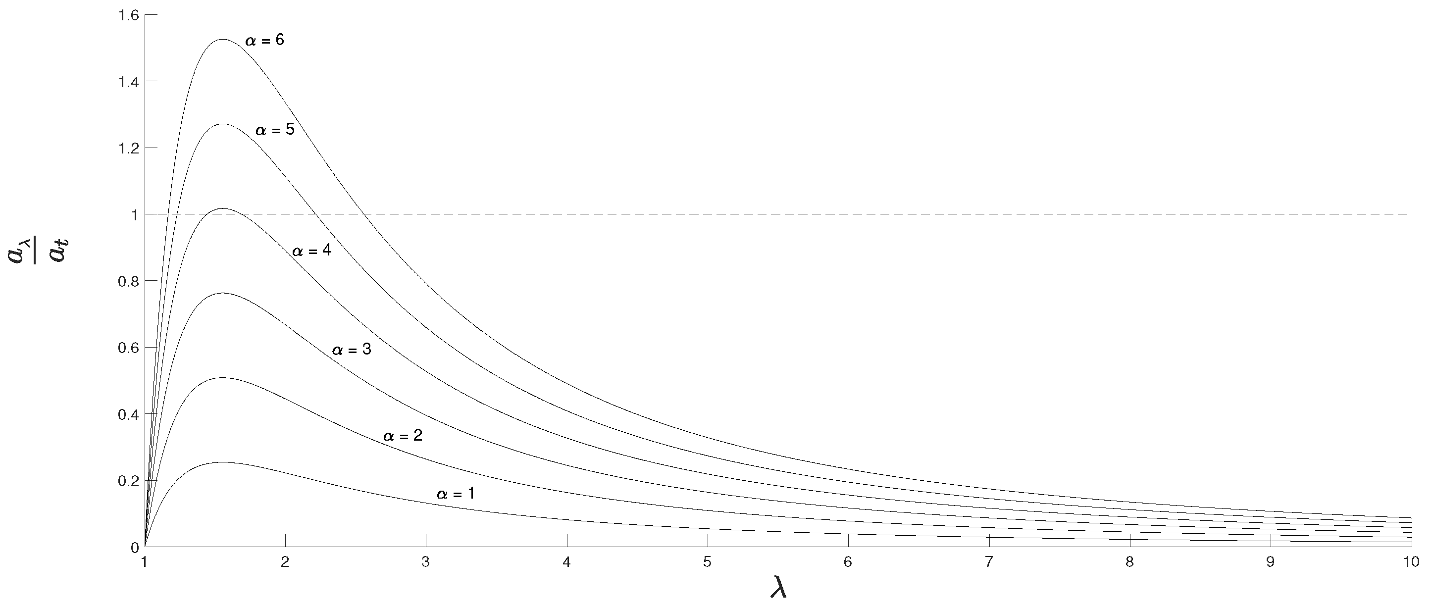
Figure 7 shows a plot of the ratio $a_{\lambda }/a_t$ as a function of $\lambda$, for ${\alpha }^{\left(tP\right)}=1,\dots ,6$. As the plots show, when ${\alpha }^{\left(tP\right)}\lesssim 3.9328$, the tidal force is stronger the tensile force at $r=\lambda /m_V$ for every value of scale factor $\lambda$, and the strong tidal forces do not permit the existence of static 't Hooft–Polyakov monopoles.

The existence of the threshold, suggested by the above heuristic argument, remains to be confirmed analytically. However, it serves as a plausibility argument for the following conjecture.

Conjecture 1.

Static 't Hooft-Polyakov monopole solution exists in non-dynamical de Sitter spacetime, in the Prasad-Sommerfeld limit, if and only if $\alpha :={(m_V/H)}^2\ge {\alpha }_0$, where ${\alpha }_0\sim O\left(1\right)$ is a constant, $m_V$ is the mass of the vector boson and H is the Hubble constant.

4. Secondary Inflation

Linde [13,17] has suggested that, although the Hubble constant H in new inflation is ∼${10}^{10}$ GeV, which is about five orders of magnitude smaller than the mass of the X boson, $m_X\sim {10}^{15}$ GeV, making ${\alpha }^{\left(GUT\right)}:={(m_X/H)}^2\sim {10}^{10}$, the inflationary background could trigger secondary inflation at a GUT monopole’s core. Linde’s argument is that, near the core, the X boson is nearly massless and the field gradients near the core of the monopole are rapidly decreased once inflation starts in the background, creating conditions suitable for the onset of secondary inflation at the core of the monopole.

In Section 4.1, we present a heuristic argument, which suggests that a weak inflationary background cannot initiate secondary inflation at the core of an $SO\left(3\right)$ 't Hooft–Polyakov monopole. Based on the heuristic analysis of secondary inflation in the 't Hooft–Polyakov monopole, we conjecture, in Section 4.2, that the secondary inflation in the GUT monopole, suggested by Linde, is infeasible.

4.1. Secondary Inflation Inside 't Hooft–Polyakov Monopole

This section presents a heuristic answer to the following question: Consider placing an initial field configuration corresponding to the Lorentzian 't Hooft–Polyakov monopole in an inflating background. Under what conditions does the inflating background drive the initial field gradients near the core of the monopole to zero?

If inflation is to drive the field gradients near the core in the initial monopole configuration to zero, then, as the monopole is stretched by inflation, the tidal force of the de Sitter background must exceed the tensile force of the monopole near the core of the monopole. Specifically, at some $\lambda \rho =\lambda \xi m_V^{-1}$, where $0<\xi <O\left(1\right)$ and $\lambda >1$, the centrifugal tidal acceleration must exceed the centripetal tensile acceleration.

Using the arguments that preceded Equations  (44) and (45), and defining the fiducial system to be the Higgs and gauge fields inside a sphere of radius $\rho =\xi m_V^{-1}$, the magnitudes of the centripetal tensile acceleration and centrifugal tidal acceleration, at $\lambda \rho =\lambda \xi m_V^{-1}$, denoted $a_{\lambda }(\xi /m_V)$ and $a_t(\xi /m_V)$, after the monopole has been stretched by a factor $\lambda$, are

$$\begin{array}{c}\hfill \begin{array}{c}{\displaystyle a_{\lambda }\left(\xi /m_V\right)=\frac{{\lambda }^2-1}{\lambda ({\lambda }^2+1)}\left(\frac{m_V}{\xi }\right)\frac{E\left(\xi m_V^{-1}\right)}{E^{\left(c\right)}\left(\xi m_V^{-1}\right)}}\hfill \\ a_t\left(\xi /m_V\right)=H^2\left({\displaystyle \frac{\lambda \xi }{m_V}}\right)\hfill \end{array}\end{array}$$

If the tidal force dominates at a distance $\lambda \rho =\lambda \xi /m_V$ from the center of the monopole for some $0<\xi <O\left(1\right),\lambda >1$, then we must have

$$\begin{array}{c}\hfill {\displaystyle a_{\lambda }\left(\xi /m_V\right)<a_t\left(\xi /m_V\right),\Rightarrow {\left(\frac{m_V}{H}\right)}^2\left[\frac{E\left(\xi m_V^{-1}\right)}{E^{\left(c\right)}\left(\xi m_V^{-1}\right)}\right]\frac{1}{{\xi }^2}<\frac{{\lambda }^2({\lambda }^2+1)}{{\lambda }^2-1}}\end{array}$$

(51)

Defining

$$\begin{array}{c}\hfill {\displaystyle q\left(\lambda \right):=\frac{{\lambda }^2({\lambda }^2+1)}{{\lambda }^2-1},k\left(\xi \right):=\frac{1}{{\xi }^2}\left[\frac{E\left(\xi m_V^{-1}\right)}{E^{\left(c\right)}\left(\xi m_V^{-1}\right)}\right]}\end{array}$$

(52)

Equation (51) becomes

$$\begin{array}{c}\hfill {\alpha }^{\left(tP\right)}k\left(\xi \right)<q\left(\lambda \right).\end{array}$$

(53)

Inequality (53) must be satisfied for the tidal acceleration to dominate tensile acceleration at a distance $\lambda \rho =\lambda \xi m_V$ when the monopole has been stretched by a factor $\lambda >1$.

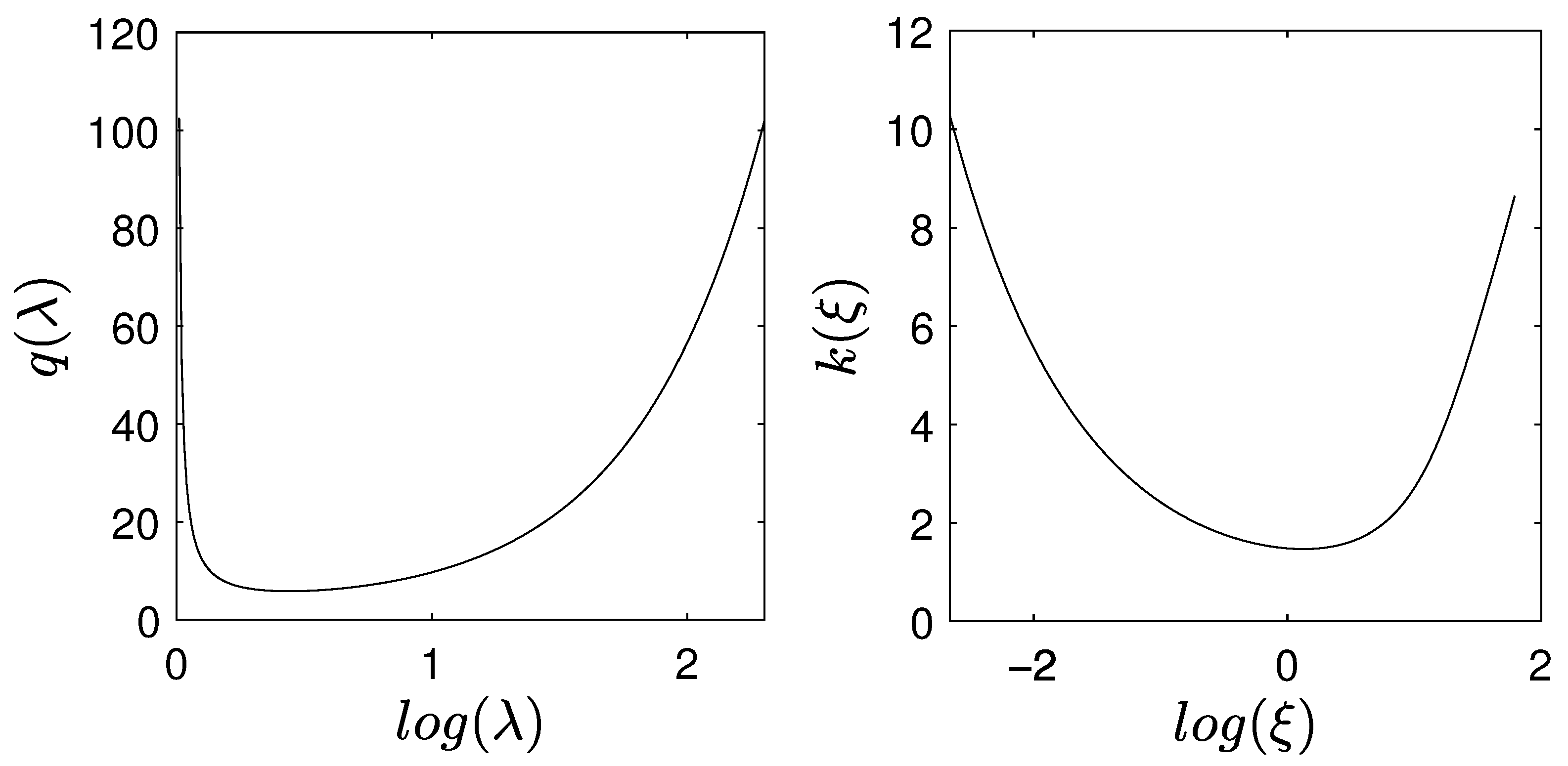
Figure 8 shows the plot of $q\left(\lambda \right)$ and $k\left(\xi \right)$. $q\left(\lambda \right)$ attains its minimum $q_{min}\sim 5.8285$ at ${\lambda }^{\ast }\sim 1.55$ and $k\left(\xi \right)$ attains its minimum value $k_{min}\sim 1.4687$ at  ${\xi }^{\ast }\sim 1.1300$.

Let ${\alpha }_0^{\left(tP\right)}=q_{min}/k_{min}\approx 3.9685$. If ${\alpha }^{\left(tP\right)}<{\alpha }_0^{\left(tP\right)}$, then

$$\begin{array}{c}\hfill {\displaystyle {\alpha }^{\left(tP\right)}<{\alpha }_0^{\left(tP\right)}=\frac{q_{min}}{k_{min}}\le \frac{q\left(\lambda \right)}{k_{min}},\mathrm{for}\mathrm{all}\lambda \ge 1\mathrm{at}{\xi }^{\ast }\sim 1.13}\end{array}$$

That is, at a distance $\rho ={\xi }^{\ast }{m}_V$ from the center, tidal acceleration is at least as large as the tensile acceleration for all $\lambda$. In other words, there is at least one distance from the center (${\xi }^{\ast }{m}_V^{-1}$) in the unstretched monopole at  which the tidal force is at least as large as the tensile force for all $\lambda >1$.

The more interesting case is when ${\alpha }^{\left(tP\right)}>{\alpha }_0^{\left(tP\right)}$. We note that $q\left(\lambda \right)$ diverges as $\lambda \to 1$. As $\lambda$ increases from 1, $q\left(\lambda \right)$ decreases until $\lambda$ reaches ${\lambda }^{\ast }$. Since ${\alpha }^{\left(tP\right)}>{\alpha }_0^{\left(tP\right)}$, there is a ${\lambda }_0\in (1,{\lambda }^{\ast })$ at which

$$\begin{array}{c}\hfill q\left({\lambda }_0\right)={\alpha }^{\left(tP\right)}{k}_{min}\end{array}$$

For any $\lambda \in ({\lambda }_0,{\lambda }^{\ast })$,

$$\begin{array}{c}\hfill q\left(\lambda \right)<q\left({\lambda }_0\right)={\alpha }^{\left(tP\right)}{k}_{min}\le {\alpha }^{\left(tP\right)}k\left(\xi \right),\mathrm{for}\mathrm{all}\xi .\end{array}$$

That is, beyond the stretching factor ${\lambda }_0$, inequality (53) is not satisfied at any $\xi$. In other words, beyond stretching factor ${\lambda }_0$, the tensile acceleration exceeds the tidal acceleration at the monopole’s core and stretching of the monopole by the inflationary background ceases. Specifically,

$$\begin{array}{c}\hfill {\displaystyle {\lambda }_0\left({\alpha }^{\left(tP\right)}\right)=\frac{1}{\sqrt{2}}{\left[(1.4687{\alpha }^{\left(tP\right)}-1)-\sqrt{2.1571{\left({\alpha }^{\left(tP\right)}\right)}^2-8.8122{\alpha }^{\left(tP\right)}+1}\right]}^{\frac{1}{2}}.}\end{array}$$

(54)

For ${\alpha }^{\left(tP\right)}\ge 628$, ${\lambda }_0\left({\alpha }^{\left(tP\right)}\right)<1$, which does not represent stretching. ${\lambda }_0\left({\alpha }^{\left(tP\right)}\right)$ decreases monotonically as ${\alpha }^{\left(tP\right)}$ increases from 4 to 627, with ${\lambda }_0\left(627\right)=1+2.12\times {10}^{-6}$.

The discussion in this section is a suggestive heuristic argument, which is useful only as a plausibility argument for the conjecture stated in Section 4.2.

4.2. Secondary Inflation in GUT Monopole

Unlike the simple $SO\left(3\right)$ gauge theory of Higgs and gauge fields, used in the construction of the 't Hooft–Polyakov monopole, the $SU\left(5\right)$ gauge theory, underlying new inflation, has Higgs, gauge and fermion fields; monopole solution arises when $SU\left(5\right)$ is broken at the GUT scale. $SU\left(5\right)$ monopole has been discussed in the literature [25]. In the following discussion, we suggest that a heuristic argument, analogous to that presented in Section 4.1, can be developed for $SU\left(5\right)$ monopoles. Again, we restrict attention to the Prasad–Sommerfeld limit in which the coupling constant in the Higgs potential—which is independent of the unified gauge coupling constant of $SU\left(5\right)$—goes to zero.

Specifically, we can consider a fiducial system comprising the fermion, gauge and Higgs fields of an $SU\left(5\right)$ monopole, within a sphere S of radius $\rho =m_X^{-1}$ from the center of the monopole, where $m_X$ is the mass of the X boson that emerges when the $SU\left(5\right)$ symmetry is broken. An estimate of the tensile force in the monopole can be obtained by regarding the increase in energy when the fiducial system is stretched by a dilatation factor $\lambda$ as the work done against a centripetal tensile force acting on the fields outside the sphere of radius $\lambda m_X^{-1}$. The tidal acceleration of the de Sitter spacetime is given by Equation (45).

The heuristic argument in Section 4.1 suggests that, for an $SO\left(3\right)$ monopole, there is a ${\alpha }_0^{\left(tP\right)}\approx 3.9685\sim O\left(1\right)$, and, for

$$\begin{array}{c}\hfill {\alpha }^{\left(tP\right)}:={\left({\displaystyle \frac{m_V}{H}}\right)}^2>{\alpha }_0^{\left(tP\right)}\end{array}$$

the tidal force of the inflationary background is too weak to continue stretching the core of the monopole beyond some small dilatation factor ${\lambda }_0$. In other words, after the soliton is stretched by a factor ${\lambda }_0$, the centripetal force dominates the tidal force, preventing further stretching; see the discussion leading up to and following Equation (54).

It seems plausible that, for the GUT monopole too, there is a ${\alpha }_0^{GUT}\sim O\left(1\right)$, and, for

$$\begin{array}{c}\hfill {\alpha }^{GUT}:={\left({\displaystyle \frac{m_X}{H}}\right)}^2>{\alpha }_0^{GUT}\end{array}$$

the tidal force of the inflationary background is too weak to continue stretching the core of an $SU\left(5\right)$ monopole beyond some small dilatation factor ${\lambda }_0^{\left(GUT\right)}$.

Based on the heuristic argument for the $SO\left(3\right)$ 't Hooft–Polyakov monopole and the speculated validity of an analogous argument for GUT monopole, we state the following conjecture.

Conjecture 2.

For ${(m_X/H)}^2\gtrsim O\left(1\right)$, where $m_X$ is the mass of the X boson and H the Hubble constant of inflationary background, secondary inflation cannot occur at the core of a GUT monopole.

Our conjecture is incompatible with Linde’s suggestion that, even at ${\alpha }^{GUT}\approx {10}^{10}$, the  inflationary background can stretch the core of a GUT monopole sufficiently to make the field gradients vanish near the core. Our conjecture can be settled with an exact analysis of the evolution of a GUT monopole in the de Sitter background that may have prevailed during the GUT phase transition.

5. Discussion

Besides the two conjectures stated above, we mention two other open problems in Section 5.1 and Section 5.2. The first problem pertains to the stability of static solitons of de Sitter spacetime. The second problem pertains to the behavior of static solitons of de Sitter spacetime when inflation ends. We also discuss below, the  impact of quantum corrections and the precision of numerical calculations presented in the paper.

5.1. Stability of the Soliton

The stability of the soliton solution described in Section 2 is an open problem. The equation satisfied by $\delta \varphi (\chi ,t)$, a small perturbation of the soliton solution, can be derived starting with Equation (2); not surprisingly, the equation for $\delta \varphi (\chi ,t)$ depends on the soliton solution, which is not available in closed form. Establishing the stability of the soliton involves showing that $\delta \varphi (\chi ,t)$ decays for arbitrary initial conditions.

5.2. Behavior of Solitons at the End of Inflation

When inflation ends, $H\to 0,\alpha \to \infty$. If spacetime becomes Lorentzian after inflation ends, it is natural to ask if a sine-Gordon soliton solution in de Sitter spacetime approaches the sine-Gordon soliton solution of flat spacetime as $H\to 0$. The answer may be nuanced. In the $H\to 0$ limit, the equation for static solutions in de Sitter spacetime—Equation (3)—does not approach the equation for static solutions in flat spacetime. At every $H\ne 0$, however small H is, Equation (3) has two singularities at $z=\pm 1$ or $u=\pm H^{-1}$. At $H=0$, the number of singularities of the equation for static solutions drops discontinuously to zero. Given the discontinuity, we may not expect the static solitons in de Sitter spacetime to morph continuously into the static solitons of flat spacetime as $H\to 0$. The behavior of static solitons in de Sitter spacetime when inflation ends warrants closer examination.

5.3. Quantum Corrections

Quantization of soliton solutions has been discussed in [26]. In the regime $\alpha :={(m/H)}^2<2$, where quantum fluctuations are important, a classical static soliton solution does not exist. In  the regime $\alpha \gtrsim 2$, the static soliton solution in de Sittter spacetime, denoted ${\varphi }_s(\chi ,t)$, can be regarded as a classical background for quantum fluctuations $\zeta (\chi ,t)$; the classical solution discussed in Section 2 can then be retained unchanged. The equation for $\zeta (\chi ,t)$, derived from Equation (2), is linear—in the small $\left|\zeta \right|$ limit—but with a damping term, which is related to the suppression of quantum fluctuations by the inflation in the background.

5.4. Numerical Calculations

The numerical calculations reported in this paper were done in MATLAB R2024b using its default double precision arithmetic. The double precision’s machine epsilon is ${\delta }_0=2.22\times {10}^{-16}$; that is, ${\delta }_0$ is the smallest number for which 1 and $1+{\delta }_0$ are regarded as different numbers in double precision arithmetic. The machine epsilon determines how closely one can approach the singularity $z=1$ in numerical investigations. We solved the differential equation using the built-in routine, ode45, which expects the second-order differential equation, such as Equation (3), to be presented as a system of first-order equations, such as

$$\begin{array}{c}\hfill \begin{array}{c}{\phi }^{\prime }\left(z\right)=\psi \left(z\right)\hfill \\ {\psi }^{\prime }\left(z\right)=-\left[{\displaystyle \frac{2z\psi \left(z\right)+\alpha sin\left(\phi \right(z\left)\right)}{(z+1)(z-1)}}\right]\hfill \end{array}\end{array}$$

If $|z-1|<{\delta }_0$, then, numerically, it is treated as $z-1=0$, and the numerical calculation leads to an overflow error. Therefore, we integrated the differential equation only up to $z=1\pm {10}^{-15}$ to ensure that the numerical calculations remained within the limits set by the machine epsilon. The differential Equation (3) was solved separately on either side of $z=1$.

None of the results presented in this paper relies on the exactness of our numerical calculations. The results of the numerical calculations have only heuristic value and serve only as plausibility arguments for the conjectures we propose.

References

1. 't Hooft, G. Magnetic monopoles in unified gauge theories. Nucl. Phys. B 1974, 79, 276–284. [Google Scholar] [CrossRef]
2. Polyakov, A.M. Particle spectrum in quantum field theory. JETP Lett. 1974, 20, 194–195. [Google Scholar]
3. Niewenhuizen, P.; Wilkinson, D.; Perry, M.J. Regular solution of 't Hooft’s magnetic monopole model in curved space. Phys. Rev. D 1976, 13, 778–784. [Google Scholar] [CrossRef]
4. Lee, K.; Nair, V.P.; Weinberg, E.J. Black holes in magnetic monopoles. Phys. Rev. D 1992, 45, 2751–2761. [Google Scholar] [CrossRef]
5. Ortiz, M.E. Curved-space magnetic monopoles. Phys. Rev. D 1992, 45, R2586–R2589. [Google Scholar] [CrossRef]
6. Breitenlohner, P.; Forgacs, P.; Maison, D. Gravitating monopole solutions. Nucl. Phys. B 1992, 383, 357–376. [Google Scholar] [CrossRef]
7. Breitenlohner, P.; Forgacs, P.; Maison, D. Gravitating monopole solutions II. Nucl. Phys. B 1995, 442, 126–156. [Google Scholar] [CrossRef]
8. Hollmann, H. On the stability of gravitating nonabelian monopoles. Phys. Lett. B 1994, 338, 181–186. [Google Scholar] [CrossRef][Green Version]
9. Lee, K.; Nair, V.P.; Weinberg, E.J. A classical instability of Reissner-Nordström solutions and the fate of magnetically charged black holes. Phys. Rev. Lett. 1992, 68, 1100–1103. [Google Scholar] [CrossRef]
10. Kibble, T.W.B. Topology of cosmic domains and strings. J. Phys. A Math. Gen. 1976, 9, 1387–1398. [Google Scholar] [CrossRef]
11. Kibble, T.W.B. Some implications of a cosmological phase transition. Phys. Rep. 1980, 67, 183–199. [Google Scholar] [CrossRef]
12. Preskill, J. Cosmological Production of superheavy magnetic monopoles. Phys. Rev. Lett. 1979, 43, 1365–1368. [Google Scholar] [CrossRef]
13. Linde, A. Monopoles as big as a universe. Phys. Lett. B 1994, 327, 208–213. [Google Scholar] [CrossRef]
14. Vilenkin, A. Topological Inflation. Phys. Rev. Lett. 1994, 72, 3137–3140. [Google Scholar] [CrossRef]
15. Basu, R.; Vilenkin, A. Evolution of topological defects during inflation. Phys. Rev. D 1994, 50, 7150–7153. [Google Scholar] [CrossRef]
16. Chen, C.; Cheng, H.; Li, X.; Zhai, X. Non-existence of topological defects during inflation beyond the critical value. Class. Quant. Grav. 1996, 13, 701–704. [Google Scholar] [CrossRef]
17. Linde, A.; Linde, D. Topological defects as seeds for eternal inflation. Phys. Rev. D 1994, 50, 2456–2468. [Google Scholar] [CrossRef]
18. Jackiw, R. Lower dimensional gravity. Nucl. Phys. B 1985, 252, 343–356. [Google Scholar] [CrossRef]
19. Teitelboim, C. Gravitation and hamiltonian structure in two spacetime dimensions. Phys. Lett. B 1983, 126, 41–45. [Google Scholar] [CrossRef]
20. Mertens, T.G.; Turiaci, G.J. Solvable models of quantum black holes: A review on Jackiw-Teitelboim gravity. Living Rev. Relat. 2023, 26, 4. [Google Scholar] [CrossRef] [PubMed]
21. Maldacena, J.; Turiaci, G.J.; Yang, Z. Two dimensional nearly de Sitter gravity. J. High Energ. Phys. 2021, 2021, 139. [Google Scholar] [CrossRef]
22. Coleman, S. Quantum sine-Gordon equation as the massive Thirring model. Phys. Rev. D 1975, 11, 2088–2097. [Google Scholar] [CrossRef]
23. Hartle, J.B. Gravity, an Introduction to Einstein’s General Relativity; Addison Wesley: San Francisco, CA, USA, 2003. [Google Scholar]
24. Prasad, M.K.; Sommerfeld, C.M. Exact classical solution for the 't Hooft monopole and the Julia-Zee dyon. Phys. Rev. Lett. 1975, 35, 760–762. [Google Scholar] [CrossRef]
25. Vachaspati, T. An attempt to construct the Standard Model with monopoles. Phys. Rev. Lett. 1996, 76, 188–191. [Google Scholar] [CrossRef]
26. Rajaraman, R. Solitons and Instantons: An Introduction to Solitons and Instantons in Quantum Field Theory; Elsevier Science Publishers B.V.: Amsterdam, The Netherlands, 1987. [Google Scholar]
27. Prabhu, N. Aspects of Soliton Physics: Existence of Static Solitons in an Expanding Universe and Quantum Soliton-Antisoliton Annihilation. Ph.D. Dissertation, MIT, Cambridge, MA, USA, 1998. [Google Scholar]
28. Whittaker, E.T.; Watson, G.N. A Course of Modern Analysis, 4th ed.; Cambridge University Press: Cambridge, UK, 1963; Reprinted. [Google Scholar]
29. Churchill, R.V. Complex Variables and Applications; International Student Edition; McGraw-Hill Book Company, Inc.: Tokyo, Japan, 1960. [Google Scholar]
30. Wrede, R.; Spiegel, M.R. Advanced Calculus, 3rd ed.; McGraw Hill: New York, NY, USA, 2010. [Google Scholar]
31. Taylor, A.E.; Mann, W.R. Advanced Calculus, 3rd ed.; John Wiley and Sons, Inc.: New York, NY, USA, 1983. [Google Scholar]
32. Bizon, P.; Mach, P. Global dynamics of a Yang-Mills field on an asymptotically hyperbolic space. Trans. Am. Math. Soc. 2017, 369, 2029–2048. [Google Scholar] [CrossRef][Green Version]
Figure 1. Sample solutions of Equation (3) in the range 1 + < z < 10 6 , where 1 + = 1 + 10 14 . The boundary conditions are φ ( 1 + ) = π / 2 , φ ( 1 + ) = ( α / 2 ) sin ( φ ( 1 + ) ) . The dotted line represents φ ( z ) 0 .
Universe 12 00119 g001
Figure 2. Solutions (solid lines) for different values of α < 2 in the range 0 z 1 : = 1 10 15 . The shown solutions correspond to φ ( 1 ) = 0.5 , 1 , 1.5 , 2 , 2.5 , 3 . φ ( 0 ) < π for all of the shown solutions. The dotted line represents φ ( z ) π .
Universe 12 00119 g002
Figure 3. Solution (solid line) for α = 1.5 and φ ( 1 10 15 ) = 1.75 , in the range 1 + 10 14 z 1 + 10 15 . The dotted line represents φ ( z ) π .
Universe 12 00119 g003
Figure 4. The three plots, in the range 0 z 1 : = 1 10 15 , show that φ ( 0 ) > π for φ ( 1 ) = 1.14218 ; φ ( 0 ) < π for φ ( 1 ) = 0.14218 ; φ ( 0 ) = π for φ ( 1 ) 0.54218 .
Universe 12 00119 g004
Figure 5. Soliton solutions (solid lines) for different values of α > 2 in the interval 0 z 10 . All of the solutions satisfy φ ( 0 ) = π and lim z φ ( z ) = 0 and are bounded at the singularity z = 1 . The plots were obtained by integrating Equation (3) separately in the intervals [ 0 , 1 ϵ ] and [ 1 + ϵ , 10 ] , where ϵ = 10 15 . The value φ ( 1 ϵ ) was chosen to ensure φ ( 0 ) = π . The dotted lines represent φ ( z ) 0 .
Universe 12 00119 g005
Figure 6. The Lorentzian sine-Gordon antikink φ S G ( x ) = 4 tan 1 ( e x ) corresponding to m = 1 (solid line). The dotted line represents φ ( z ) π .
Universe 12 00119 g006
Figure 7. a λ / a t as a function of λ for α ( t P ) = 1 , , 6 . α ( t P ) is abbreviated to α in the labels shown in the plots. The plots (solid lines) show that, for α ( t P ) < 3.9328 , the tidal forces are too strong— a λ / a t < 1 —and do not allow static 't Hooft–Polyakov monopole to exist in de Sitter spacetime. The dashed line represents a λ / a t 1 .
Universe 12 00119 g007
Figure 8. Plots of k ( ξ ) and q ( λ ) .
Universe 12 00119 g008
Disclaimer/Publisher’s Note: The statements, opinions and data contained in all publications are solely those of the individual author(s) and contributor(s) and not of MDPI and/or the editor(s). MDPI and/or the editor(s) disclaim responsibility for any injury to people or property resulting from any ideas, methods, instructions or products referred to in the content.