A Tailored Deep Learning Network with Embedded Space Physical Knowledge for Auroral Substorm Recognition: Validation Through Special Case Studies

Abstract

The dynamic morphological characteristics of the auroral oval serve as critical diagnostic indicators for auroral substorm recognition, with each pixel in ultraviolet imager (UVI) data carrying different physical implications. Existing deep learning approaches often overlook the physical properties of auroral images by directly transplanting generic models into space physics applications without adaptation. In this study, we propose a visual–physical interactive deep learning model specifically designed and optimized for accurate auroral substorm recognition. The model leverages the significant variation in auroral morphology across different substorm phases to guide feature extraction. It integrates magnetospheric domain knowledge from space physics through magnetic local time (MLT) and magnetic latitude (MLAT) embeddings and incorporates cognitive features derived from expert eye-tracking data to enhance spatial attention. Experimental results on substorm sequences recognition demonstrate satisfactory performance, achieving an accuracy of 92.64%, precision of 90.29%, recall of 93%, and F1-score of 91.63%. Furthermore, several case studies are presented to illustrate how both visual and physical characteristics contribute to model performance, offering further insight into the spatiotemporal complexity of auroral substorm recognition.

1. Introduction

The auroral substorm is a visual manifestation of the magnetospheric substorm. When the Earth’s magnetosphere is severely disturbed, it happens naturally [1,2]. This is a natural consequence of the complex interactions between the solar wind and the Earth’s magnetosphere. Specifically, it is an energy transformation and dissipation in the magnetosphere. Physicists have been interested in understanding the causes of substorms [1,3,4,5,6,7,8,9]. Auroral substorms can be observed by auroral images captured by the ultraviolet imager (UVI) [10], which is equipped on the Polar satellite. It can collect hundreds of millions of UVI images during its operation. To explore the occurrence and dynamic variations of auroral substorms, scientists face a monumental challenge and undertaking in extracting substorm data from thousands upon thousands of UVI images.

The foundational work for the study of auroral substorms was initiated by [11,12], who manually identified the onset of substorms from multiple Ultraviolet Imager (UVI) images. These early efforts provided the data necessary for further research into the dynamics of auroral substorms. Scholars have since investigated how space physics parameters influence the occurrence and evolution of substorms, emphasizing their sensitivity to specific disturbances in the magnetosphere [4,7,13,14,15,16].

For example, variations in geomagnetic indices such as AE, AL, and AU have been found to correspond to the intensity of disturbances within the magnetosphere during a substorm event [17,18]. Furthermore, the relationship between Pi2 magnetic pulsations and auroral substorms has been explored [19], suggesting that these oscillations may offer insights into substorm dynamics. Reactions to solar wind and Interplanetary Magnetic Field (IMF) in different auroral substorm phases are also a hot topic [20]. These methods typically involve using simple regression equations to model the relationships between space physics parameters and substorm phases. However, since each substorm event is unique, these equations may not be universally applicable or accurate for all cases, highlighting the complexity and variability of auroral substorms.

In the past decades, machine learning methods have shown their formidable feature extraction power in space science. Many methods have been developed for modeling or processing auroral images. In the early stages of auroral image processing, Murphy et al. developed a method [21] to estimate auroral breakup timing using auroral image sequences. Their approach involved extracting spatial features such as brightness and distribution patterns from all-sky images, followed by the application of statistical models for time series analysis to predict the precise moment of auroral breakup. The Morphology Adaptive Threshold Method [22] was employed using varying thresholds to enhance the feature extraction ability of auroral images. The authors employed the Adaptive Local Binary Patterns (ALBPs) algorithm and Gabor filtering [23] to extract distinctive morphological features from the auroral images. The Local Feature Descriptor (LFD) [24] was also used to represent auroral textures.

With the rise in clustering algorithms, techniques like SFCM [25], K-Nearest Neighbors (KNN) [26], and distributed weighted KNN [27] were introduced for extracting distinct features, so that different aurora patterns and images can be easily discriminated. Zhong et al. proposed a multi-feature Latent Dirichlet Allocation (AI-MFLDA) method [28] for aurora image classification, in which grayscale, structural, and texture features are uniformly converted into one-dimensional histograms and modeled in multiple independent spaces to achieve low-dimensional representation and efficient classification of aurora images. The use of dimensionality reduction methods, such as Low-rank Matrix Factorization [29] became prevalent to better represent auroral images. Based on these different auroral image features, Hidden Markov Models [30,31] and Support Vector Machine (SVM) [32,33] were applied to classify auroral images or auroral substorm sequences. These early traditional machine learning techniques gradually gave way to neural networks and deep learning methods as they became more prominent in computer vision.

Since 2015, neural and deep learning networks have emerged as dominant approach in auroral image processing. Scholars have progressively applied models to various tasks, including classification, segmentation, retrieval, and prediction. For instance, a two-layer Restricted Boltzmann Machine (RBM) [34] was used to learn the distribution of auroral oval boundaries. Other neural architectures, such as the Backpropagation (BP) network, Radial Basis Function Neural Networks (RBF), Generalized Regression Neural Networks (GRNNs) have been applied to model auroral oval intensity and structure [35]. Researchers have also introduced improved convolutional auto-encoder models to capture subtle and latent auroral features. Convolutional Neural Networks (CNNs) have been widely adopted for their strong performance in extracting spatial features from various auroral morphologies [36,37,38,39,40]. Similarly, some researchers have integrated traditional machine learning methods, such as hash coding and metric learning, with Convolutional Neural Networks (CNNs) to obtain more discriminative and effective features for classification [41,42]. Building on this, a saliency-weighted Mask R-CNN was proposed to enhance auroral image retrieval by focusing on the most informative regions of the images [43]. In 2021, researchers further advanced the field using a Generative Adversarial Network (GAN) to capture higher-level, improving generalization in classification tasks [44]. For sequence modeling, Long Short-Term Memory (LSTM) networks have proven effective in capturing temporal characteristics in auroral image sequences, enabling improved substorm detection and evolution prediction [45]. More recently, Transformer-based models have also been introduced to extract and classify features from auroral images, leveraging their ability to capture long-range dependencies and contextual information [46,47]. In addition to the supervised methods mentioned above, an unsupervised learning approach using clustering techniques to detect auroral breakups from all-sky image sequences, demonstrating the potential of label-free methods for scalable auroral event detection [48]. However, these methods rarely incorporate domain knowledge and expert cognition in the modeling process. To address this limitation, we explore a new direction that integrates domain expertise directly into the model design.

The most intuitive way to show the visual cognition of space physicists is by recording their eye movement information when they select the auroral substorm sequences from UVI images. In this paper, we propose a novel and tailored visual–physical interactive model based on spatial physics knowledge and experts’ eye movement information to accurately identify auroral substorms. The main contributions are described as follows:

1.

We developed a novel space knowledge embedding module called the Visual–Physical Interaction (VPI) module, which simultaneously incorporates eye movement patterns and scientific knowledge. The core of this module is the MLT-MLAT embedding, inspired by the physical characteristics and unique data attributes of auroral substorms. This method is based on the Altitude Adjusted Corrected Geomagnetic Coordinates (AACGM) system. The MLT-MLAT embedding approach closely aligns with space physics knowledge, offering an enhanced representation of auroral substorm features.

2.

The eye movement patterns are considered a type of empirical knowledge in this work. As a result, an auroral substorm eye movement dataset is established by collecting eye movement data from space physicists. Auroral substorm events used in this study are comprehensive, including various types of auroral substorm sequences. We analyze these eye movement data and generate the eye movement patterns for various auroral substorms. In addition, we generate visual maps using an Eye Movement Pattern Prediction (EMPP) module, which learns from the eye movement patterns of experts.

3.

We thoroughly analyze and compare the variation patterns of the Interplanetary Magnetic Field (IMF) and the AE index observed between auroral substorms that were correctly identified (easy samples) and those that were misclassified (difficult samples). By identifying these differences, we gain a deeper understanding of the inherent challenges and complex factors in auroral substorm recognition.

2. Data Collection and Process

2.1. Auroral Substorm Data

The data acquisition used a 2D snapshot camera on the Polar satellite to continuously capture auroral oval images (200 × 228 pixels) in the pre-midnight sector. To minimize dayglow effects, we analyzed 180 days of northern winter observations from December 1996 to May 1997, with capture intervals ranging from 0.5 to 3 min. Each image was georegistered using the Altitude Adjusted Corrected Geomagnetic Coordinates (AACGM) system, resulting in standardized 241 × 241 pixel grids.

A typical substorm progresses through three distinct phases. As shown in Figure 1, the growth phase exhibits a quiet, homogeneous arc structure with minimal luminosity variation. Substorm onset is marked by localized brightening within pre-existing midnight sector arcs. During the expansion phase, this brightened region shows pronounced luminosity enhancement and equatorward boundary expansion. The recovery phase commences when the enhanced auroral emissions gradually dissipate, eventually restoring the quiet-state configuration. To ensure a consistent and physically meaningful definition of substorm onset, we adopted the commonly used criteria introduced by Frey et al. [11]: (1) a clear, localized brightening of the aurora near the equatorward boundary of the oval, (2) poleward and azimuthal expansion sustained for at least 20 min, and (3) a minimum 30 min separation between successive events.

In this work, the onset list published by Kan Liou in 2010 [12] was used to select auroral substorm sequences. This list was constructed based on visual inspection of Polar UVI images and is consistent with the criteria described by Frey et al. [11]. Additionally, previous studies [49] suggest that a substorm onset is often accompanied by an increase in the AE index of more than 100 nT within a ±10 min window. Therefore, our study employs a multi-source identification strategy. Specifically, the determination of substorm onset was based on three complementary indicators: (1) morphological changes in the auroral oval observed in UVI images: a clear, localized brightening of the aurora; (2) enhancements in auroral intensity as visualized in keograms; and (3) rapid AE index increases: an increase in the AE index of more than 100 nT within a ±10 min window.

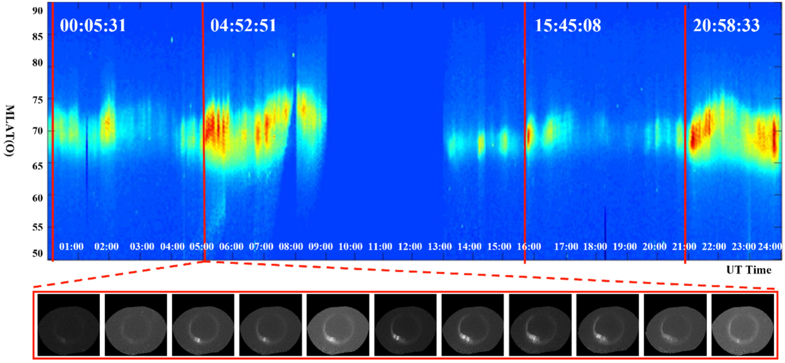
The keogram is an important visualization tool for the auroral substorm recognition in the space physics field. Figure 2 displays the keogram and corresponding auroral substorm sequence at 04:52:51. When the auroral substorm occurs, the high energy flux will be released. Red lines identify each auroral substorm onset seen on the keogram. It can be seen that on this day, there are several moments of energy flux growth only according to keogram diagram, but according to the above-mentioned principle of determining the three onset moments, this paper selects four substorm onset moments on this day.

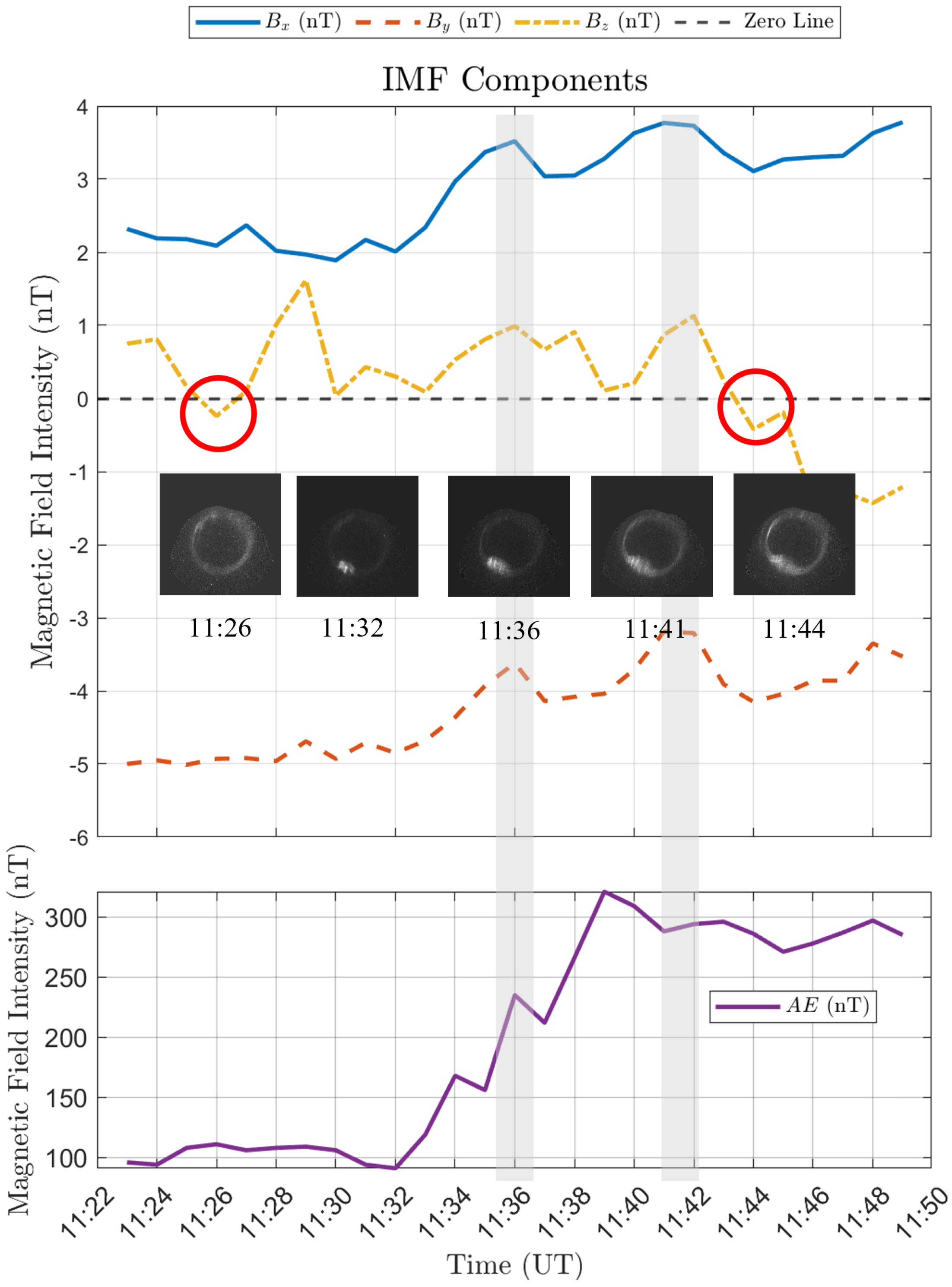
Figure 3 illustrates an auroral substorm event that occurred on 30 January 1997, supporting the validity of the data selection strategy employed in this study. At 11:26 UT, the Bz component of the IMF shifted from northward to southward. Six minutes later, at 11:32 UT, the UVI image captured a brightening on the nightside auroral oval (Substorm onsets). Meanwhile, the AE index exhibited two significant surges [4,7,14,50,51], and an increase in the AE index of more than 100 nT within a ±10 min window [49]. During this period, IMF Bz exhibited a significant positive value. As the substorm entered the expansion phase, the IMF components Bx, By, and Bz experienced a sudden positive increase at 11:36 UT. Concurrently, the UVI image showed the brightened region on the auroral oval expanding within the magnetic local time (MLT) sector.

At 11:41 UT, IMF By and IMF Bz began to rise further, but within two minutes, IMF Bz transitioned again from positive to negative, marking a shift from northward to southward. At this point, the auroral brightening extended significantly poleward, with a rapid expansion in both magnetic local time and latitude. This substorm event featured two instances of southward and sudden northward Bz increases. The first shift occurred before the onset phase and aligns with the findings of “the two-step evolution of auroral acceleration at substorm onset” [52]. The second shift occurred during the expansion phase, coinciding with the rapid poleward expansion of the auroral brightening, consistent with previous studies on southward IMF Bz during the expansion phase. The observed variations in these physical parameters align well with existing research [53,54,55,56,57,58,59,60], providing additional validation of our data selection approach.

Based on the determination of substorm onset and the criteria and domain knowledge described above, the data selection principles are as follows:

1.

The UVI images in the growth phase are within 10–20 min before the onset.

2.

The UVI images of the expansion phase and the recovery phase are within 30–90 min after the onset.

3.

The auroral substorm sequences are discontinuous due to occasional observation gaps. As a result, some UVI frames in a sequence may appear completely dark and were excluded. Only those sequences exhibiting clear auroral evolution consistent with the above criteria were retained.

4.

Each sequence must include images within the onset and expansion phase. Consequently, the processed substorm sequences contain 5 to 26 qualified images.

To further validate the reliability of our event selection and labeling, multiple domain experts were independently invited to examine the selected auroral substorm sequences. We clearly inform them that they need to judge based on the standards put forward by Frey [11]. The high degree of agreement among their assessments, as reflected in the consistency of their eye-tracking fixation maps (shown in Figure 4), provides additional evidence that the selected sequences clearly exhibit physical signatures associated with substorm onset. As shown in

Table 1. The auroral substorm dataset.

Date	December 1996–February 1997	March 1997–May 1997	December 1997
Substorm	290	73	27
Non-Substorm	120	130	-
	Training dataset	test dataset

, a total of 390 substorm sequences were selected, and 250 non-substorm sequences were selected randomly during the time of non-substorm occurrence. These data include most auroral substorm types. According to common sense and observation criterion described above, the data selection principles include the length distribution of all substorm sequences, as shown in Figure 5, whether they are substorm or non-substorm sequences, the length distribution of the data in the training set, and the test set showing a consistent trend. This crucial data guarantees the verification of the performance of the proposed model.

2.2. Auroral Substorms Eye Movement Data

Auroral substorms are primarily classified by their morphological characteristics, combined with quantitative analysis of variations in space physics parameters. This morphology-driven methodology fundamentally depends on expert visual interpretation by space physicists. To operationalize this expertise, we utilize eye-tracking technology to capture the visual attention patterns of specialists during systematic auroral substorm identification. These empirically grounded visual signatures provide domain-specific priors that significantly enhance the precision of automated substorm detection algorithms.

A total of 15 participants (aged 20–40 years with normal or corrected-to-normal vision) were recruited for the auroral substorm eye-tracking experiment. All participants were researchers (faculty or graduate students) actively engaged in auroral physics. We conducted eye-tracking data collection using the Eyelink 1000 Plus system. During trials, auroral image sequences were randomly displayed, and participants classified each sequence as either containing a substorm event or not. If uncertain during initial viewing, participants could review sequences multiple times before final judgment. Each subject participated in 20–30 groups of substorm sequence recognition experiments. Since the differences in eye movement information can be disregarded in this task-oriented experiment under a unified judgment criterion, they ensure the similarity of the eye movement information of the experts when they observe the same substorm sequence.

The fixation positions of the subjects exhibit considerable variation across different stages of the substorm sequence. The eye movement visualizations represent the actual eye movement patterns recorded from experts when observing auroral substorm data. Figure 4 shows that the eye movement patterns during the expansion phase of all substorm sequences differ significantly from those during other phases of substorm images. However, there is no clear pattern in the eye movement patterns during different stages of non-substorm sequences. From the growth phase to the recovery phase, the fixation positions of subjects show a transition from dispersion to aggregation. Before onset, the fixation positions are distributed randomly. However, during the expansion phase and recovery phase, the fixation positions become relatively concentrated. The majority of fixations are found between 60 and 80 MLAT in geomagnetic latitude and between 18 and 4 MLT in magnetic local time. This pattern aligns with the morphological development of the substorm sequence. It suggests that the experts’ visual patterns change with the dynamic changes in auroral oval intensity and position.

To leverage the visual eye movement information, it is essential to transform the eye movement data from a 2D point into a visual representation. Hence, fixation data were visually depicted in the form of fixation maps. These visual maps were generated using the fixation positions, and are detailed as follows:

Step 1: Utilize the eye fixation point data from all experts to generate fixation maps for each substorm sequence. For the i-th expert observing the k-th substorm sequence, a sparse fixation map $E{M}_i^k(x,y)$ is defined as follows:

$$E{M}_i^k(x,y)=\sum _{p=1}^m\delta (x-x_p,y-y_p)$$

(1)

where $(x_p,y_p)$ denotes the coordinates of the p-th fixation point, and m is the total number of fixations. The aggregated fixation map $F{M}^k$ is then obtained by summing the fixation maps across all N experts as follows:

$$F{M}^k=\sum _{i=1}^{N}E{M}_i^k$$

(2)

Step 2: A Gaussian spatial filter $C_f$ is constructed and convolved with $F{M}^k$ to produce a continuous visual map $I_V$, which emphasizes salient regions of expert visual attention as follows:

$$I_V=F{M}^k\ast C_f$$

(3)

Figure 6 illustrates representative samples of auroral substorm sequences alongside their corresponding visual maps.

Table 2. The auroral substorm eye movement dataset.

Date	December 1996–February 1997	March 1997–May 1997	December 1997
Fixation maps	336	generate	58
Visual maps	336	generate	58
Subjects	15

summarizes the eye movement dataset used in this paper, comprising both empirically collected eye movement data and visual maps computationally generated by our Eye Movement Pattern Prediction (EMPP) model.

2.3. Data Preprocessing

Given the inherent variability in auroral substorm durations and imaging protocols, raw substorm sequences exhibit significant temporal heterogeneity. To standardize inputs for deep neural network training, we implement temporal normalization using the frame processing operation defined in Equation (4):

$$S_p=\left\{\begin{array}{cc}\langle s_1,\dots ,s_i,\underset{p-i}{\underbrace{s_i,\dots ,s_i}}\rangle \hfill & i<p\hfill \\ \langle s_1,\dots ,s_p\rangle \hfill & i\ge p\hfill \end{array}\right.$$

(4)

where $S_p$ denotes the normalized sequence of predetermined length p, derived from the original sequence S containing i frames. The normalization threshold p is empirically set based on the mode of sequence lengths in our dataset. This procedure either (1) pads shorter sequences by duplicating the final frame when $i<p$, or (2) truncates excess frames beyond the index p for longer sequences.

The expansion phase is widely recognized as the key signature for identifying auroral substorms in the field of space physics, whereas accurately defining the end of the recovery phase remains challenging. Consequently, our preprocessing strategy ensures that all training sequences contain complete expansion phase signatures, while allowing for the acceptable exclusion of late-stage recovery dynamics. The omission of frames in the recovery phase is considered tolerable. Corresponding visual attention maps undergo the same temporal normalization to maintain spatiotemporal alignment with the image sequences, yielding coordinated pairs of image and visual map sequences.

3. Method

The proposed method comprises two modules: the Eye Movement Pattern Prediction (EMPP) module and the Visual–Physical Interactive (VPI) module. The EMPP module is designed to simulate the eye movement behaviors of experts and generate visual maps. Guided by spatial physics principles observed during substorm events, we utilize the VPI module to learn the dynamic spatiotemporal relationships between expert visual maps and substorm images, thereby distinguishing substorm characteristics from ordinary auroral features and ultimately achieving accurate identification of substorm events. Figure 7 illustrates the overall pipeline of the proposed method. Initially, in the EMPP model, auroral images are processed through a standard embedding layer followed by a series of Transformer encoder layers to generate the corresponding visual maps. Then, these generated visual maps, together with the corresponding auroral images, are used as input to the VPI module for automated substorm recognition. In the VPI module, each frame in a sequence, consisting of an auroral image and its corresponding visual map, is first encoded using MLT-MLAT embedding, which performs spatial partitioning and encoding along Magnetic Local Time (MLT) and Magnetic Latitude (MLAT) dimensions. The resulting features are processed by multiple Transformer encoder layers to extract high-dimensional patch representations. Patch features derived from the auroral images and visual maps are concatenated within each MLT-MLAT block to obtain fused patch features. These features are further concatenated in temporal order to construct frame-wise sequence features. Finally, these sequence-level features are input into a multi-layer perceptron (MLP) classifier to perform substorm identification. The following sections describe the detailed architecture of these two modules.

3.1. Eye Movement Pattern Prediction (EMPP) Module

We employed a simple network built on Transformer architecture [61] to produce visual maps that balance reasoning time and the accuracy of the EMPP module. The EMPP module is designed based on the visual transformer (ViT) network [62]. It provides a built-in saliency to gain insight into what the model is focused on, which is what we want the model to learn from the visual maps. As shown in Figure 8, the auroral images are fed into the ResNet50 model [63] to extract image features. Subsequently, the obtained image features are input into a standard ViT network to locate visual fixation regions corresponding to different substorm stages. Additionally, a recovery head is employed to map salient regions on the substorm images and generate visual maps.

To facilitate the network in better distinguishing and learning the eye movement patterns of different stages of substorm sequences, the EMPP module does not consider the temporality of the sequences. The data are shuffled and input into the network in the form of individual images for training. Specifically, when an auroral image of size 241 × 241 × 3 is fed into the module, image features of size 4096 × 512 are first extracted using the ResNet50-ViT backbone. These features are then reshaped through a permutation (permute) layer and an unflatten operation to a tensor of size 512 × 64 × 64. Subsequently, a normalization layer and a 2D convolutional layer are applied to reduce the channel dimensionality. Finally, an upsampling operation is performed to restore the spatial resolution, producing a visual map with the same size as the input image.

The Cross-Entropy (CE) [64] and Linear Correlation Coefficient (CC) [65] serve as the loss function for the EMPP module. In Equation (5), $cov\left(\right)$ represents the covariance function, ${\delta }_O$ and ${\delta }_G$, respectively, represent the standard deviation of the predicted visual map O and the ground truth G.

$$CC(O,G)=cov(O,G)/{\delta }_O\ast {\delta }_G$$

(5)

We employed 336 auroral substorm sequences (December 1996–February 1997), each paired with expert-validated visual maps, for training the EMPP model. The training configuration utilizes several hyperparameters to optimize model performance. The model is trained for 400 epochs with an initial learning rate of 0.0001. A batch size of 10 is employed. To stabilize training and mitigate exploding gradients, a gradient clipping margin of 0.5 is applied. The learning rate is scheduled to decay by a factor of 0.5 every 50 epochs to facilitate gradual convergence. Optimization is performed using Stochastic Gradient Descent (SGD) [66] with a momentum coefficient of 0.9. Following successful training convergence, the optimized EMPP architecture was deployed across our complete observational dataset, generating visual maps of 390 substorm sequences and 250 non-substorm sequences. These synthesized visual maps subsequently served as inputs to our VPI module for automated substorm recognition.

3.2. Visual–Physical Interaction (VPI) Module

3.2.1. MLT-MLAT Embedding

Physicists typically transform auroral substorm images into magnetic local time (MLT) and geomagnetic latitude (MLAT) coordinates for analysis. In this coordinate system, we can discern the dynamic changes in bright spots on the auroral oval in a uniform standard. Unlike natural images or images from other professional fields, as shown in Figure 9, conventional partitioning methods often divide the bright spot region into multiple patches, making it difficult to capture the complete evolution process of the bright spots. However, the dynamic changes in bright spots on the auroral oval are crucial indicators for judging substorms. We design a novel image patch embedding way named MLT-MLAT Embedding to divide and embedding the auroral substorm images. Geomagnetic latitude and magnetic local time have different spatial physics implications. Therefore, this paper partitions and encodes auroral substorm images separately along these two directions. Studies suggest that substorms generally occur on the dusk and night sides of the Earth, but there is no definite geomagnetic timing for their onset. Therefore, magnetic local time (MLT) is divided into four major zones, representing noon, morning, dusk, and night sector, respectively. The circles of different colors represent different ranges of geomagnetic latitudes.

The embedding of MLT patches follows the same approach as that of regular visual transformers. As for MLAT patches, since the size of each patch varies due to different ranges of geomagnetic latitudes, a fully connected operation is utilized to map their embedding dimensions to the same dimensionality as the MLT embedding. The details are as explained in Equations (6)–(8). Assuming that after the MLAT partitioning operation, the patches are denoted as $M{p}_{89}$, $M{p}_{78}$, $M{p}_{67}$, $M{p}_{56}$, where each patch size is flattened into a vector, $d1-d4$ represent the dimensions of each MLAT patch vector.

$$\left\{\begin{array}{c}\hfill M{p}_{89}^{d1}=flatten\left(M{p}_{89}\right)\\ \hfill M{p}_{78}^{d2}=flatten\left(M{p}_{78}\right)\\ \hfill M{p}_{67}^{d3}=flatten\left(M{p}_{67}\right)\\ \hfill M{p}_{56}^{d4}=flatten\left(M{p}_{56}\right)\end{array}\right.$$

(6)

Then, the vectors of different MLAT patches are concatenated to get the MLAT feature with $4\ast (d1+d2+d3+d4)$ dimension.

$$Mp=concat(M{p}_{89}^{d1},M{p}_{78}^{d2},M{p}_{67}^{d3},M{p}_{56}^{d4})$$

(7)

Similarly to the operations of normal patch embedding, we employ two normalization layers and one linear mapping layer to encode the MLAT feature $Mp$. The MLAT embedding feature $Me$ can be obtained.

$$Me={\displaystyle \frac{((\frac{Mp-{\mu }_1}{{\sigma }_1}\ast {\gamma }_1+{\beta }_1)\ast w_d+b_d)-{\mu }_2}{{\sigma }_2}}\ast {\gamma }_2+{\beta }_2$$

(8)

${\mu }_1$ and ${\sigma }_1$ represent the mean and variance of $Mp$, and ${\sigma }_1$ and ${\gamma }_1$ are learnable parameter vectors with $d1+d2+d3+d4$ dimensions. Meanwhile, ${\sigma }_2$ and ${\gamma }_2$ also are learnable parameter vectors with d dimensions. They are used to scale and shift the normalized results. ${\beta }_1$ is a very small constant to avoid division by zero. w and b represent the weight matrix and bias for linear mapping, respectively. d denotes the mapping dimension. The value of d is consistent with the dimension of the MLT patch embedding.

Specifically, in the VPI module, the MLT-MLAT Embedding operations described above are applied to both the auroral substorm image sequences and their corresponding visual map sequences. We partition the input data cube along the time dimension and perform embedding across multiple consecutive frames. This method preserves temporal dependencies between frames while encoding spatial relationships within Magnetic Local Time (MLT) and Magnetic Latitude (MLAT). This process yields four types of embedding features: $E_{MLT}^{AS}$ and $E_{MLAT}^{AS}$ for the auroral substorm images, $E_{MLT}^{VS}$ and $E_{MLAT}^{VS}$ for the visual maps. All four embeddings share the same shape of 10 × 5 × 4 × 1024, where the first dimension corresponds to the batch size. The second dimension represents the temporal channel, meaning that during cube partitioning, two consecutive frames are grouped at a time. Thus, for a 10-frame sequence, five temporal segments are generated. The third dimension denotes the number of spatial patches, and the fourth is the feature embedding dimension.

3.2.2. Architecture of the VPI Module

The detail of feature transmit in the VPI module is displayed in Figure 10, where the b represents batch size, the $f=framenumber/tubletsize$, p denotes the patch number, and d is the embedding dimension. After MLT-MLAT Embedding operations, Positional encoding are added to each embedding features, resulting in a feature dimension of 10 × 5 × 5 × 1024. To obtain more compact and representative features, a convolutional operation is applied to reduce the dimensionality to 10 × 5 × 1024. This yields four sets of token representations: $Toke{n}_{MLT}^{AS}$ and $Toke{n}_{MLAT}^{AS}$ for the auroral substorm images, $Toke{n}_{MLT}^{AS}$ and $Toke{n}_{MLAT}^{AS}$ for the visual maps.These tokens are further refined using a Transformer encoder and then concatenated to form the final MLAT-MLT feature representation: $T_{AS}$ for the auroral substorm images and $T_{VS}$ for the visual maps, both with a feature dimension of 10 × 5 × 2048.

Subsequently, a max pooling layer followed by a Transformer encoder is applied to further reduce the dimensionality and enhance the semantic representation. This yields compressed representations of size 10 × 3 × 1024 for the auroral substorm images and 10 × 3 × 128 for the visual maps. These two representations are then concatenated along the feature axis in a frame-wise manner, resulting in a fused feature tensor of size 10 × 3 × 1152. This fused feature captures both the spatial characteristics of the auroral morphology (through MLAT and MLT embeddings) and the enhanced visual semantics derived from the generated visual maps.

To perform auroral substorm recognition, the fused features are first passed through an average pooling layer to reduce the dimensionality to 10 × 1 × 576. A Transformer encoder is then employed to model temporal dependencies between the auroral substorm token $T_{AS}$ and the visual token $T_{VS}$. The resulting token $T_{AV}$, which integrates both physical spatial knowledge and visual cues, is fed into a multi-layer perceptron (MLP) for classification. The final output is a probability vector of shape 10 × 2, indicating the likelihood of each sequence being a substorm or non-substorm event.

In addition, the Cross-Entropy (CE) [64] is employed as the loss function for training the VPI module. There are 290 substorm sequences and 120 non-substorm sequences from December 1996 to February 1997 that were used to train the module, and 100 substorm sequences and 130 non-substorm sequences from March to May 1997 and December 1997 were used as test data to verify the performance of the model.

The model training process incorporates several critical hyperparameters to facilitate effective optimization and ensure convergence. The training is performed over 100 epochs, with an initial learning rate set to 1 × 10⁻⁴ and a batch size of 10, which determines the number of samples utilized for each parameter update. Optimization is carried out using Stochastic Gradient Descent (SGD) [66] with a momentum coefficient of 0.9 to accelerate convergence and mitigate oscillations. To enhance training stability and avoid gradient explosion, gradient clipping with a threshold of 0.5 is employed. Additionally, a learning rate decay schedule is implemented, reducing the learning rate by a factor of 0.5 every 20 epochs. Collectively, these hyperparameter choices contribute to a robust and efficient training regime.

4. Experimental Results

All experiments were conducted in a computational environment utilizing CUDA 12.0, PyTorch 1.10, and Python 3.7, accelerated by an NVIDIA RTX 4090 GPU.

4.1. EMPP Results

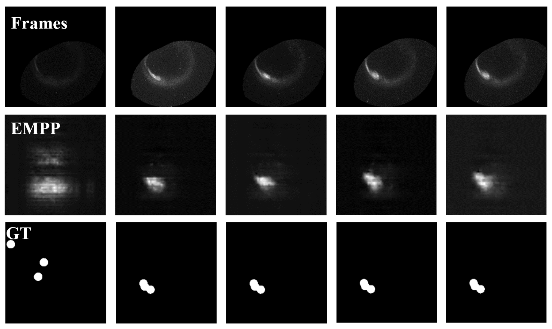
Figure 11 demonstrates the visual attention maps generated through our EMPP framework, organized in three comparative rows: (a) representative frames from auroral substorm sequences (top), (b) EMPP-predicted visual maps (middle), and (c) expert-annotated ground truth visual attention patterns (bottom). Quantitative visual inspection reveals that our predictions exhibit strong congruence with expert annotations in both spatial distribution and relative saliency magnitude of critical substorm features.

4.2. VPI Results

We employ four principal classification metrics for quantitative performance evaluation: Accuracy, Precision, Recall, and F1-score. These measures are operationally defined as follows:

• Accuracy: The proportion of correct predictions relative to total predictions, reflecting overall classification correctness.
• Precision: The ratio of true positive predictions to all positive classifications, quantifying prediction reliability with higher values indicating fewer false alarms.
• Recall (Sensitivity): The percentage of actual positive cases correctly identified, measuring detection completeness where higher values correspond to fewer missed events.
• F1-score: The harmonic mean balancing precision and recall, particularly critical for evaluating performance on imbalanced datasets where strict precision-recall tradeoffs exist.

$$\mathrm{Accuracy}={\displaystyle \frac{TP+TN+FP+FN}{TP+TN}}$$

(9)

$$\mathrm{Precision}={\displaystyle \frac{TP}{TP+FP}}$$

(10)

$$\mathrm{Recall}={\displaystyle \frac{TP}{TP+FN}}$$

(11)

$$\mathrm{F}1-\mathrm{score}=2\ast {\displaystyle \frac{Precision\ast Recall}{Precision+Recall}}$$

(12)

where $TP$ stands for True Positive, $TN$ for True Negative, $FP$ for False Positive, and $FN$ for False Negative, while Accuracy gives an overall evaluation of the model, it may be misleading in cases of imbalanced data, where the model could predict the majority class well but fail to identify the minority class. The F1-score serves as the primary performance indicator for auroral substorm detection, where both false negatives (missed substorms) and false positives (spurious detections) carry significant consequences in space weather monitoring applications.

4.2.1. Ablation Experiments

The MLT-MLAT embedding is a method proposed for substorm sequence recognition based on domain-specific spatial physics knowledge. To minimize the influence of feature fusion strategies on model performance, a set of experiments was conducted using only auroral input sequences to validate the effectiveness of the proposed MLT-MLAT embedding.

The results show that both MLT and MLAT embeddings significantly preserve the integrity of bright spot regions on the auroral oval in the

Table 3. The experiment results on different embedding methods.

Embedding Methods	Accuracy	Precision	Recall	F1-Score
MLAT-MLT	0.9177	0.8584	0.97	0.9108
MLAT	0.9087	0.8349	0.94	0.8843
MLT	0.8918	0.8151	0.97	0.8858

. However, during periods of intense geomagnetic activity, these regions may span multiple magnetic local times and geomagnetic latitudes. In such cases, using either embedding independently may fail to maintain spatial coherence. By jointly applying MLT and MLAT embeddings, the two methods provide complementary spatial information, allowing the model to better capture auroral structures and thereby achieve optimal performance.

To assess the contribution of eye-tracking-based visual information, we conducted a series of ablation experiments with different combinations of model inputs.

Table 4. The experiment results on different inputs.

Model Inputs	Accuracy	Precision	Recall	F1-Score
Visual+MLAT-MLT	0.8918	0.9310	0.81	0.8663
Substorm+ MLAT-MLT	0.9177	0.8584	0.97	0.9108
Visual+Substorm +MLAT-MLT	0.9264	0.9192	0.91	0.9146

presents the results for three settings: (1) Visual+MLAT-MLT, which includes only the eye movement attention maps; (2) Substorm+MLAT-MLT, which uses only the original auroral substorm sequences; and (3) Visual+Substorm+MLAT-MLT, which combines all three modalities.

The results demonstrate that each input modality contributes uniquely to model performance. Specifically, the Substorm+MLAT-MLT input yields the highest recall (0.97), indicating strong sensitivity to substorm detection. However, this high recall is accompanied by a relatively low precision (0.8584), implying an increased rate of false positives. In contrast, the Visual+MLAT-MLT input achieves the highest precision (0.9310), suggesting that visual attention maps derived from eye-tracking data effectively suppress background noise and highlight relevant auroral regions.

When all three modalities are combined (Visual+Substorm+MLAT-MLT), the model achieves a balanced performance with a recall of 0.91 and a precision of 0.9192, resulting in the highest F1-score (0.9146). This confirms that integrating visual attention maps enhances feature discriminability and complements the temporal patterns embedded in auroral substorm sequences.

These findings underscore the value of incorporating expert-driven eye-tracking information, which offers human–attention–informed priors that significantly enhance the robustness and overall accuracy of the model.

As shown in Figure 11, in a substorm sequence, the significant regions predicted by the EMPP module in the visual map are also concentrated. Compared to the original auroral substorm images, the visual maps effectively remove background interference, allowing the network to capture better and learn the typical features of substorm sequences. Compared to the single-input model, where each model excels in one metric while performing poorly in others, the model that combines visual maps and original substorm sequences inputs achieves a more balanced performance and satisfactory results across all four metrics.

4.2.2. Comparative Experiments

To establish empirical validation of our model’s performance, we first compared its effectiveness with recent popular video recognition methods based on the Transformer architecture using the proposed substorm image sequence dataset. The comparison methods are Vit [62] and Video-Swin [67] published in 2021, Video-FocalNet [68], and DualFormer [69] proposed in 2023. Secondly, we also compared its performance with related works [25] on substorm sequence recognition. The specific experimental results are shown in

Table 5. The experiment results on different models.

Models	Accuracy	Precision	Recall	F1-Score
Vit-3d’2021	0.9134	0.8846	0.92	0.9020
Video-Swin-tiny’2021	0.8304	0.8	0.81	0.8050
Video-Swin-small’2021	0.6391	0.5702	0.75	0.6479
Video-FocalNet’2023	0.9091	0.8692	0.93	0.8986
DualFormer-tiny’2023	0.8609	0.8384	0.83	0.8342
Yang’s’2013	-	0.4928	0.9198	0.6417
DCSD- C3D’2022	-	0.5701	0.9771	0.7201
DCSD-R3D’2022	-	0.5573	0.9733	0.7088
DCSD-R2Plus1D’2022	-	0.5788	0.9733	0.7259
EMSF-R2Plus1D’2023	0.8826	0.8462	0.88	0.8627
EMSF-C3D’2023	0.9087	0.8911	0.9	0.8955
Ours	0.9264	0.9029	0.93	0.9163

. This comparative analysis evaluates the efficacy of the proposed visual–physical interactive deep learning model in capturing critical spatiotemporal patterns characteristic of auroral substorm evolution.

To further evaluate the generalizability of our model in real-world scenarios, we conducted an additional experiment using an unfiltered, continuous 10-day UVI dataset from January 1998. These dataset naturally contains substorm events and includes no manually excluded samples. First, we fed the full dataset into the trained Eye Movement Pattern Prediction (EMPP) module to generate corresponding visual attention maps. Next, we employed previously saved weights of the Visual–Physical Interactive (VPI) module at different training epochs. Following a procedure similar to that of [70], we segmented the data into sequences of 10 consecutive UVI images along with their corresponding visual maps. These sequences were then passed through a partially trained VPI model, which is capable of identifying sequences lacking significant auroral variation—such as dark or non-informative images. This allowed for automated filtering of irrelevant samples without human intervention. The remaining sequences, consistent in format with the main study’s dataset, were input into the fully trained VPI model for substorm detection. The detection results were compared against manually identified substorm onset times, following the standard criteria described in our methodology. On this raw dataset, the model achieved an identification accuracy of approximately 88%.This experiment demonstrates that our framework retains strong performance even when applied to unfiltered, real-world data, supporting the robustness and practical applicability of the proposed method for auroral substorm identification.

5. Discussion

In this study, we focus specifically on four space physics parameters published in NASA’s CDAWeb (https://cdaweb.gsfc.nasa.gov/ (accessed on 30 July 2025)) that are closely linked to auroral substorm dynamics: the three components of the Interplanetary Magnetic Field (Bx, By, Bz) and the auroral electrojet index (AE). We use 1-minute-averaged OMNI IMF and AE observations. The space physics data analyzed in this study span from 10 min prior to auroral substorm onset to the conclusion of the auroral substorm sequence, as defined by the duration of UVI substorm images. This temporal window ensures the inclusion of critical features from the growth, expansion, and recovery phases of the substorm. By encompassing both pre-onset and post-event dynamics, this methodology enables a comprehensive examination of the interactions between space weather parameters and auroral substorm progression. Such an approach is pivotal for identifying key patterns and understanding the processes driving substorm evolution.

5.1. Case Example: Successful Cases

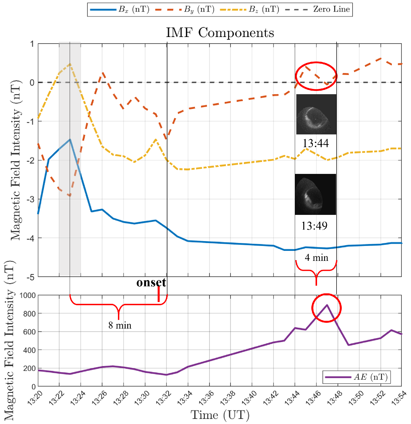
Figure 12 represents a correctly identified substorm event that occurred on 1 March 1997, at 13:30 UT. This event is classified as a major auroral substorm. We analyzed the energy dynamics observed on the auroral oval from Polar UVI observations alongside variations in IMF components and the AE index. Eight minutes prior to onset, the IMF Bz component exhibited a brief southward turning. At the same time, IMF Bx and By remained southward, with Bx showing a sharp decrease in magnitude and By exhibiting a numerical increase. Four minutes later, By also underwent a brief directional reversal. During the expansion phase, intense auroral activity was observed from 13:44 UT to 13:48 UT, and IMF By showed an increasing trend. Subsequently, within two minutes, IMF By turned southward again, transitioning from positive to negative. This period of vigorous auroral activity was visually confirmed in UVI imagery, and the AE index peaked concurrently, reflecting heightened geomagnetic disturbances.

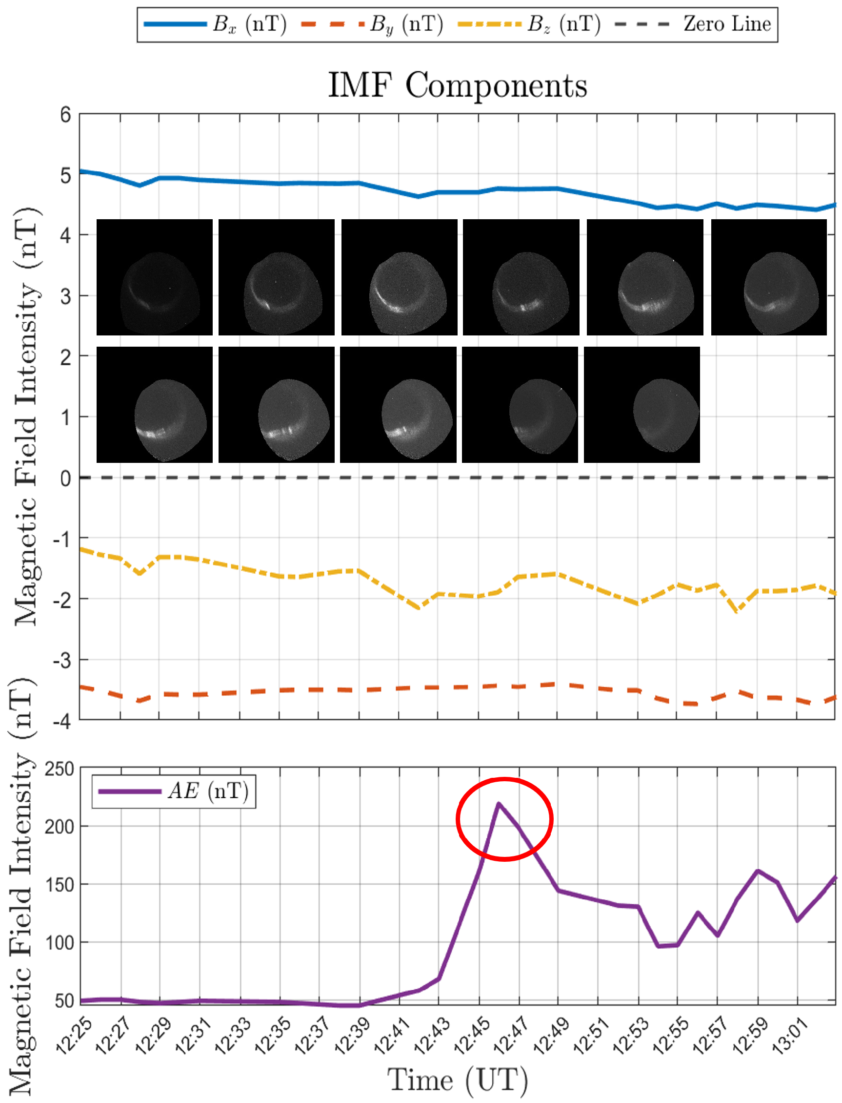
Figure 13 illustrates a correctly identified moderate auroral substorm event that occurred on 13 December 1997, at 12:19 UT. Throughout the substorm, IMF Bz and By remained consistently southward, while Bx remained persistently northward. During the expansion phase, the AE index reached its peak, corresponding to intensified auroral activity and underscoring the relationship between these space physics parameters and substorm dynamics.

5.2. Case Example: Failure Cases

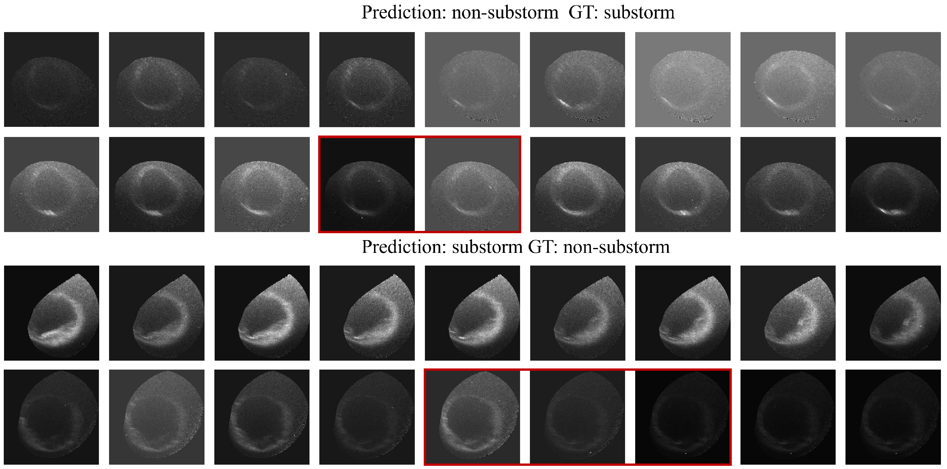
Although our model has performed well in substorm identification tasks, there are still a small number of failure cases. Figure 14 shows examples of recognition errors in two scenarios.

When the substorm activity is weak, the bright spot area on the auroral arc does not change significantly, and the model is prone to misclassify the substorm sequence as a non-substorm sequence. At the same time, due to the influence of the spatial environment on the imaging equipment, there is a tendency for the intensity of the auroral arc to suddenly weaken in the image during the substorm expansion stage, as shown in the red box in the second row of Figure 14. This phenomenon can also lead to incorrect identification of substorm events by the model. In addition, not all strong auroral activity corresponds to a substorm event; the key indicators are the appearance, expansion, and dissipation of bright spots on the auroral arc. The sequence shown in the third row of Figure 14 did not experience a substorm event, although there was extreme auroral activity. The sequence shown in the fourth row misled the model into believing that there were changes in the bright spots, and thus it was incorrectly identified as a substorm. In summary, in subsequent work, we need to focus on studying how to capture and measure subtle changes in auroral arcs to improve the accuracy of substorm identification.

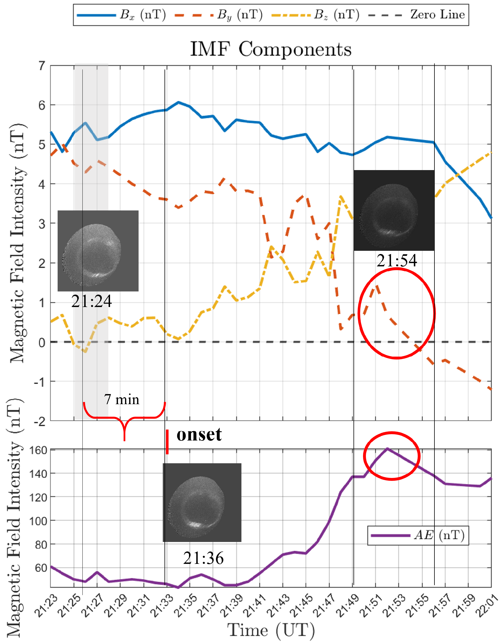
Figure 15 illustrates an incorrectly identified auroral substorm event that occurred on 2 March 1997, at 21:33 UT. This event is categorized as a moderate substorm. Before the onset, IMF Bz briefly shifted from northward to southward. At the same time, both IMF Bx and By were southward. The IMF Bx showed a sudden decrease, while By exhibited an increase. However, the AE index exhibited minimal variation during this period. During the expansion phase, between 21:49 UT and 21:55 UT, IMF By increased, followed by a reversal to a negative (southward) direction in the next two minutes. During this period, the AE index reached its peak, reflecting significant auroral activity associated with this phase of the substorm.

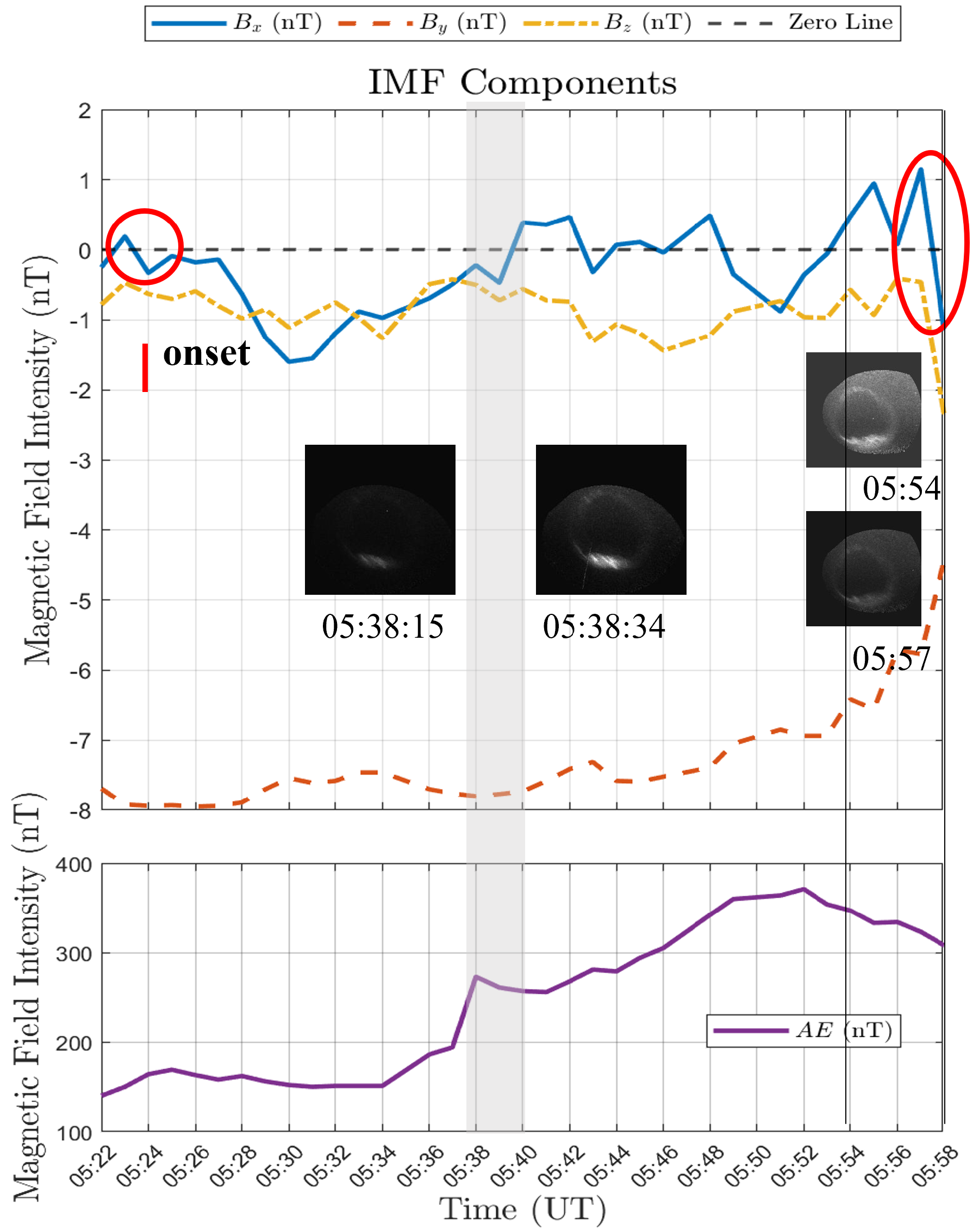
Figure 16 illustrates an incorrectly identified auroral substorm event that occurred on 28 May 1997, at 05:22 UT. This substorm is classified as a large substorm. As shown in the figure, two minutes prior to the onset, IMF Bx briefly shifted from northward to southward. Meanwhile, IMF By and Bz remained southward and stabilized at relatively steady values. Additionally, the AE index showed minimal variation during this period. During the expansion phase, at 05:38 UT, the AE index experienced a sudden increase. However, from the UVI image taken at 05:38:15 UT, no significant auroral activity was observed on the auroral oval. By 05:38:34 UT, bright spots on the auroral oval expanded noticeably. IMF Bx exhibited an increase followed by a reversal from negative to positive, changing from southward to northward. In the recovery phase, from 05:54 UT to 05:57 UT, as the bright spots on the auroral oval gradually returned to a quieter state, IMF Bx increased and then shifted from positive to negative, changing from northward to southward.

5.3. Comparative Analysis of Success and Failure Cases

The comparative analysis of successful and failure cases reveals distinct patterns in both physical parameters and auroral image features. In successful cases, the interplanetary magnetic field (IMF) components [71,72], particularly Bz [73,74,75,76], exhibit clear directional shifts or changes in magnitude prior to substorm onset [77]. These are often accompanied by a sharp increase in the AE index [78,79] during the expansion phase [80]. The physical variations show a strong temporal correlation with the observed auroral activity. Visually, the auroral sequences in these cases present a well-defined evolution through the typical substorm phases: growth, expansion, and recovery, characterized by dynamic changes in the brightness and structure of auroral arcs. In contrast, failure cases often involve weaker or ambiguous changes in the IMF components and minimal response in the AE index, which reduces the model’s confidence in identifying substorm events. Visually, these sequences may show limited auroral variation or be affected by environmental noise and atypical brightness fluctuations, such as sudden dimming or irregular bright spots that are not consistent with the physical indicators. These discrepancies emphasize the importance of reliable physical trends and clear visual cues for improving the accuracy of substorm identification.

Our proposed integration of spatially meaningful physical knowledge, specifically the MLAT-MLT embedding, offers a new direction to improve the model accuracy. In addition, the incorporation of eye-tracking-based visual maps enhances the expression of critical regions within auroral images, helping the model to better focus on informative features. Furthermore, the failure cases analyzed also reflect the limitations of our current model design, emphasizing the need for incorporating more explicit representations of the fundamental physical processes governing substorm evolution, such as data-informed physical constraints or learned differential equations, in future work to further improve model performance.

6. Conclusions

For special domains, integrating domain knowledge into deep learning networks is one of the key factors in improving network performance. In this paper, eye movement data from multiple space physics experts were collected, and based on this, the eye movement visual patterns of space physics experts in identifying substorm events were explored. Furthermore, inspired by space physics principles, an embedding method for auroral substorm images was designed, and a substorm recognition network was developed based on expert visual eye movement patterns. The experimental results presented in the paper also demonstrate the effectiveness of the proposed approach. With the proposed method, potential substorm events can be efficiently identified from a large volume of auroral UVI images, significantly reducing the workload for experts. Although the proposed method is currently applicable only to substorm event recognition, the MLT-MLAT embedding strategy introduced in this study is generalizable to all types of UVI images and can support the analysis of other space weather phenomena.

Through the analysis of correctly and incorrectly identified substorm samples, we examined the variations in the IMF components (Bx, By, Bz) and the AE index at different phases of the substorm. Additionally, for the incorrectly identified samples, we analyzed the reasons for failure based on changes in image intensity and other factors. These investigations offer valuable guidance for refining the substorm identification methodology. The study highlights that relying solely on unimodal data for analyzing space weather events is unreliable. A robust and accurate prediction framework requires the integration of multiple data modalities and diverse observational instruments.

References

1. Akasofu, S.I. The development of the auroral substorm. Planet. Space Sci. 1964, 12, 273–282. [Google Scholar] [CrossRef]
2. Li, L.Y.; Cao, J.B.; Zhou, G.C.; Li, X. Statistical roles of storms and substorms in changing the entire outer zone relativistic electron population. J. Geophys. Res. Space Phys. 2009, 114, A12214. [Google Scholar] [CrossRef]
3. Lui, A.T.Y. Tutorial on geomagnetic storms and substorms. IEEE Trans. Plasma Sci. 2000, 28, 1854–1866. [Google Scholar] [CrossRef]
4. Lyons, L.R. A new theory for magnetospheric substorms. J. Geophys. Res. 1995, 100, 19069–19081. [Google Scholar] [CrossRef]
5. McPherron, R.L. Magnetospheric substorms. Rev. Geophys. 1979, 17, 657–681. [Google Scholar] [CrossRef]
6. Newell, P.; Gjerloev, J.W. Substorm and magnetosphere characteristic scales inferred from the supermag auroral electrojet indices. J. Geophys. Res. 2011, 116, A12232. [Google Scholar] [CrossRef]
7. Newell, P.; Liou, K.; Gjerloev, J.; Sotirelis, T.; Wing, S.; Mitchell, E. Substorm probabilities are best predicted from solar wind speed. J. Atmos. Sol.-Terr. Phys. 2016, 146, 28–37. [Google Scholar] [CrossRef]
8. Pudovkin, M. Physics of Magnetospheric Substorms: A Review. In Magnetospheric Substorms; Kan, J.R., Potemra, T.A., Eds.; American Geophysical Union: San Francisco, CA, USA, 2013; pp. 28–37. [Google Scholar]
9. Liu, Z.Y.; Zong, W.G.; Zong, Q.G.; Wang, J.S.; Yu, X.Q.; Wang, Y.F.; Zou, H.; Fu, S.Y.; Yue, C.; Hu, Z.J.; et al. The Response of Auroral-Oval Waves to CIR-Driven Recurrent Storms: FY-3E/ACMag Observations. Universe 2023, 9, 213. [Google Scholar] [CrossRef]
10. Brittnacher, M.; Spann, J.; Parks, G. Auroral observations by the polar Ultraviolet Imager (UVI). Adv. Space Res. 1997, 20, 1037–1042. [Google Scholar] [CrossRef]
11. Frey, H.U.; Mende, S.B. Substorm onsets as observed by IMAGE-FUV. J. Geophys. Res. Space Phys. 2004, 104, A10304. [Google Scholar]
12. Liou, K. Polar Ultraviolet Imager observation of auroral breakup. J. Geophys. Res. Space Phys. 2010, 115, A12219. [Google Scholar] [CrossRef]
13. Akasofu, S.I. The roles of the north-south component of the interplanetary magnetic field on large-scale auroral dynamics observed by the DMSP satellite. Planet. Space Sci. 1975, 23, 1349–1354. [Google Scholar] [CrossRef]
14. Caan, M.N.; McPherron, R.L.; Russell, C.T. Characteristics of the association between the interplanetary magnetic field and substorms. J. Geophys. Res. 1977, 82, 4837–4842. [Google Scholar] [CrossRef]
15. Freeman, M.P.; Morley, S.K. A minimal substorm model that explains the observed statistical distribution of times between substorms. Geophys. Res. Lett. 2004, 31, L12807. [Google Scholar] [CrossRef]
16. Henderson, M.G.; Reeves, G.D.; Belian, R.D.; Murphree, J.S. Observations of magnetospheric substorms occurring with no apparent solar wind/IMF trigger. J. Geophys. Res. 1996, 101, 10773–10791. [Google Scholar] [CrossRef]
17. Vennerstrom, S.; Friis-Christensen, E.; Troshichev, O.A.; Andersen, V.G. Comparison between the polar cap index, PC, and the auroral electrojet indices AE, AL, and AU. J. Geophys. Res. Space Phys. 1991, 96, 101–113. [Google Scholar] [CrossRef]
18. Alberti, T.; Faranda, D.; Consolini, G.; De Michelis, P.; Donner, R.V.; Carbone, V. Concurrent Effects between Geomagnetic Storms and Magnetospheric Substorms. Universe 2022, 8, 226. [Google Scholar] [CrossRef]
19. Sutcliffe, P.R. Substorm onset identification using neural networks and Pi2 pulsations. Ann. Geophys. 1997, 15, 1257–1264. [Google Scholar] [CrossRef]
20. Wang, H.; Lühr, H. Effects of solar illumination and substorms on auroral electrojets based on CHAMP observations. J. Geophys. Res. Space Phys. 2021, 126, e2020JA028905. [Google Scholar] [CrossRef]
21. Murphy, K.R.; Miles, D.M.; Watt, C.E.J.; Rae, I.J.; Mann, I.R.; Frey, H.U. Automated Determination of Auroral Breakup during the Substorm Expansion Phase Using All-Sky Imager Data. J. Geophys. Res. Space Phys. 2014, 119, 1414–1427. [Google Scholar] [CrossRef]
22. Yang, X.; Gao, X.B.; Tao, D.C.; Li, X. Improving level set method for fast auroral oval segmentation. IEEE Trans. Image Process. 2014, 23, 2854–2865. [Google Scholar] [CrossRef]
23. Fu, R.; Gao, X.B.; Jian, Y.J. Patchy Aurora Image Segmentation Based on ALBP and Block Threshold. In Proceedings of the 20th International Conference on Pattern Recognition, Istanbul, Turkey, 23–26 August 2010; IEEE: Piscataway, NJ, USA, 2010; pp. 3380–3383. [Google Scholar]
24. Niu, C.; Zhang, J.; Wang, Q.; Liang, J. Weakly Supervised Semantic Segmentation for Joint Key Local Structure Localization and Classification of Aurora Image. IEEE Trans. Geosci. Remote Sens. 2018, 56, 7133–7146. [Google Scholar] [CrossRef]
25. Yang, Q.J.; Liang, J.M. A method for automatic identification of substorm expansion phase onset from UVI images. Chin. J. Geophys. 2013, 56, 1435–1447. [Google Scholar]
26. Syrjäsuo, M.; Donovan, E. Analysis of auroral images: Detection and tracking. Geophysica 2002, 38, 3–14. [Google Scholar]
27. Li, Y.; Jiang, N. An Aurora Image Classification Method based on Compressive Sensing and Distributed WKNN. In Proceedings of the 2018 IEEE 42nd Annual Computer Software and Applications Conference (COMPSAC), Tokyo, Japan, 23–27 July 2018; pp. 347–354. [Google Scholar]
28. Zhong, Y.; Huang, R.; Zhao, J.; Zhao, B.; Liu, T. Aurora Image Classification Based on Multi-Feature Latent Dirichlet Allocation. Remote Sens. 2018, 10, 233. [Google Scholar] [CrossRef]
29. Yang, X.; Gao, X.B.; Tao, D.C.; Li, X.; Han, B.; Li, J. Shape-constrained sparse and low-rank decomposition for auroral substorm detection. IEEE Trans. Neural Netw. Learn. Syst. 2015, 27, 32–46. [Google Scholar] [CrossRef]
30. Yang, Q.; Liang, J.; Hu, Z.; Zhao, H. Auroral Sequence Representation and Classification Using Hidden Markov Models. IEEE Trans. Geosci. Remote Sens. 2012, 50, 5049–5060. [Google Scholar] [CrossRef]
31. Sado, T.; Kataoka, R.; Tanaka, Y. Substorm Onset Prediction from Auroral Image Sequences Using Deep Learning; ESSOAr: Online, 2022. [Google Scholar]
32. Hu, Z.J.; Lian, H.F.; Zhao, B.R.; Han, B.; Zhang, Y.S. Automatic Identification of Auroral Substorms Based on Ultraviolet Spectrographic Imager Aboard Defense Meteorological Satellite Program (DMSP) Satellite. Universe 2023, 9, 412. [Google Scholar] [CrossRef]
33. Syrjäsuo, M.; Donovan, E.; Qin, X.; Jackel, B.; Liang, J.; Voronkov, I.; Connors, M.; Spanswick, E.; Milling, D.; Frey, H. Automatic Classification of Auroral Images in Substorm Studies. In Proceedings of the 8th International Conference on Substorms (ICS-8), University of Calgary, Banff, AB, Canada, 27–31 March 2006; pp. 309–313. [Google Scholar]
34. Han, B.; Gao, X.B.; Liu, H. Auroral Oval Boundary Modeling Based on Deep Learning Method. In 2015 International Conference on Intelligent Science and Big Data Engineering; Springer: Berlin, Germany, 2015; pp. 96–106. [Google Scholar]
35. Hu, Z.J.; Han, B.; Lian, H.F. Modeling of ultraviolet auroral oval boundaries based on neural network technology. Sci. Sin. Technol. 2019, 49, 531–542. [Google Scholar] [CrossRef]
36. Wang, Q.; Fang, H.; Li, B. Automatic Identification of Aurora Fold Structure in All-Sky Images. Universe 2023, 9, 79. [Google Scholar] [CrossRef]
37. Shang, Z.; Yao, Z.; Liu, J.; Xu, L.; Xu, Y.; Zhang, B.; Guo, R.; Wei, Y. Automated Classification of Auroral Images with Deep Neural Networks. Universe 2023, 9, 96. [Google Scholar] [CrossRef]
38. Wang, F.; Yang, Q.J. Classification of auroral images based on convolutional neural network. Chin. J. Polar Res. 2018, 30, 123–131. [Google Scholar]
39. Clausen, L.B.N.; Nickisch, H. Automatic classification of auroral images from the Oslo Auroral THEMIS (OATH) data set using machine learning. J. Geophys. Res. Space Phys. 2018, 123, 5640–5647. [Google Scholar] [CrossRef]
40. Sado, P.; Clausen, L.B.N.; Miloch, W.J.; Nickisch, H. Transfer learning aurora image classification and magnetic disturbance evaluation. J. Geophys. Res. Space Phys. 2022, 127, e2021JA029683. [Google Scholar] [CrossRef] [PubMed]
41. Endo, T.; Matsumoto, M. Aurora Image Classification with Deep Metric Learning. Sensors 2022, 22, 6666. [Google Scholar] [CrossRef]
42. Gu, G.H.; Huo, W.H.; Su, M.Y.; Fu, H. Asymmetric Supervised Deep Discrete Hashing Based Image Retrieval. J. Electron. Inf. Technol. 2021, 43, 3530–3537. [Google Scholar]
43. Yang, X.; Wang, N.; Song, B.; Gao, X. Aurora Image Search with a Saliency-Weighted Region Network. IEEE Trans. Geosci. Remote Sens. 2020, 58, 12630–12643. [Google Scholar] [CrossRef]
44. Hu, Z.J.; Han, B.; Zhang, Y.; Lian, H.; Wang, P.; Li, G.; Li, B.; Chen, X.C.; Liu, J.J. Modeling of ultraviolet aurora intensity associated with interplanetary and geomagnetic parameters based on neural networks. Space Weather 2021, 19, e2021SW002751. [Google Scholar] [CrossRef]
45. Jiang, X.; Zhang, T.; Moen, J.I.; Wang, H. Aurora evolution prediction using ConvLSTM. Earth Space Sci. 2023, 10, e2022EA002721. [Google Scholar] [CrossRef]
46. Lian, J.; Liu, T.; Zhou, Y. Aurora Classification in All-Sky Images via CNN–Transformer. Universe 2023, 9, 230. [Google Scholar] [CrossRef]
47. Zhong, Y.; Yi, J.; Ye, R.; Zhang, L. Cross-Station Continual Aurora Image Classification. IEEE Trans. Geosci. Remote Sens. 2024, 62, 1–12. [Google Scholar] [CrossRef]
48. Partamies, N.; Dol, B.; Teissier, V.; Juusola, L.; Syrjäsuo, M.; Mulders, H. Auroral breakup detection in all-sky images by unsupervised learning. Ann. Geophys. 2024, 42, 103–115. [Google Scholar] [CrossRef]
49. Ding, W.Z.; Cao, J.B.; Aimin, D. Statistical analysis of substorm onsets determined by geomagnetic indices. Chin. J. Space Sci. 2010, 30, 17–22. [Google Scholar] [CrossRef]
50. Kullen, A.; Ohtani, S.; Karlsson, T. Geomagnetic signatures of auroral substorms preceded by pseudobreakups. J. Geophys. Res. 2019, 114, A04201. [Google Scholar] [CrossRef]
51. McPherron, R.L.; Russell, C.T.; Aubry, M.P. Satellite studies of magnetospheric substorms on August 15, 1968: 9. Phenomenological model for substorms. J. Geophys. Res. 1973, 78, 3131–3149. [Google Scholar] [CrossRef]
52. Maimaiti, M.; Kunduri, B.; Ruohoniemi, J.M.; Baker, J.B.H.; House, L.L. A Deep Learning-Based Approach to Forecast the Onset of Magnetic Substorms. Space Weather 2019, 17, 1534–1552. [Google Scholar] [CrossRef]
53. Gromova, L.I.; Forster, M.; Feldstein, Y.I.; Ritter, P. Characteristics of the electrojet during intense magnetic disturbances. Ann. Geophys. 2018, 36, 1361–1391. [Google Scholar] [CrossRef]
54. Huang, T.; Luhr, H.; Wang, H. Global characteristics of auroral Hall currents derived from the Swarm constellation: Dependencies on season and IMF orientation. J. Geophys. Res. 2017, 122, 378–392. [Google Scholar] [CrossRef]
55. Huang, T.; Luhr, H.; Wang, H.; Xiong, C. The relationship of high-latitude thermospheric wind with ionospheric horizontal current, as observed by CHAMP satellite. Ann. Geophys. 2017, 35, 1249–1268. [Google Scholar] [CrossRef]
56. Pulkkinen, T.I.; Tanskanen, E.L.; Viljanen, A.; Partamies, N.; Kauristie, K. Auroral electrojets during deep solar minimum at the end of solar cycle 23. J. Geophys. Res. 2011, 116, A04207. [Google Scholar] [CrossRef]
57. Shue, J.H.; Kamide, K. Effects of solar wind density on auroral electrojets. Geophys. Res. Lett. 2001, 28, 2181–2184. [Google Scholar] [CrossRef]
58. Singh, A.K.; Rawat, R.; Pathan, B.M. On the UT and seasonal variations of the standard and SuperMAG auroral electrojet indices. J. Geophys. Res. 2013, 118, 5059–5067. [Google Scholar] [CrossRef]
59. Vennerstrom, S.; Moretto, T. Monitoring auroral electrojet with satellite data. Space Weather 2013, 11, 509–519. [Google Scholar] [CrossRef]
60. Wang, H.; Luhr, H.; Ridley, A.; Ritter, P.; Yu, Y. Storm time dynamics of auroral electrojets: CHAMP observation and the space weather modeling framework comparison. Ann. Geophys. 2008, 26, 555–570. [Google Scholar] [CrossRef]
61. Vaswani, A.; Shazeer, N.; Parmar, N.; Uszkoreit, J.; Jones, L.; Gomez, A.N.; Kaiser, Ł.; Polosukhin, I. Attention Is All You Need. In Proceedings of the 31st Conference on Neural Information Processing Systems (NeurIPS), Long Beach, CA, USA, 4–9 December 2017; pp. 5998–6008. [Google Scholar]
62. Dosovitskiy, A.; Beyer, L.; Kolesnikov, A.; Weissenborn, D.; Zhai, X.; Unterthiner, T.; Houlsby, N. An image is worth 16x16 words: Transformers for image recognition at scale. arXiv 2020, arXiv:2010.11929. [Google Scholar]
63. He, K.; Zhang, X.; Ren, S.; Sun, J. Deep Residual Learning for Image Recognition. In Proceedings of the 2016 IEEE Conference on Computer Vision and Pattern Recognition (CVPR), Las Vegas, NV, USA, 27–30 June 2016; pp. 770–778. [Google Scholar]
64. Bishop, C.M. Pattern Recognition and Machine Learning; Springer: New York, NY, USA, 2006. [Google Scholar]
65. Bylinskii, Z.; Judd, T.; Oliva, A.; Torralba, A.; Durand, F. What do different evaluation metrics tell us about saliency models? IEEE Trans. Pattern Anal. Mach. Intell. 2019, 41, 740–757. [Google Scholar] [CrossRef]
66. Robbins, H.; Monro, S. A stochastic approximation method. Ann. Math. Stat. 1951, 22, 400–407. [Google Scholar] [CrossRef]
67. Liu, Z.; Ning, J.; Cao, Y.; Wei, Y.; Zhang, Z.; Lin, S.; Hu, H. Video Swin Transformer. arXiv 2021, arXiv:2106.13230. [Google Scholar] [CrossRef]
68. Wasim, S.T.; Khattak, M.U.; Naseer, M.; Khan, S.; Shah, M.; Khan, F.S. Video-FocalNets: Spatio-Temporal Focal Modulation for Video Action Recognition. In Proceedings of the IEEE International Conference on Computer Vision, Paris, France, 2–6 October 2023. [Google Scholar]
69. Liang, Y.; Zhou, P.; Zimmermann, R.; Yan, S. DualFormer: Local-Global Stratified Transformer for Efficient Video Recognition. In Proceedings of the IEEE International Conference on Computer Vision, Paris, France, 2–6 October 2023. [Google Scholar]
70. Sado, P.; Clausen, L.B.N.; Miloch, W.J.; Nickisch, H. Substorm onset prediction using machine learning classified auroral images. Space Weather 2023, 21, e2022SW003300. [Google Scholar] [CrossRef]
71. Wild, J.A.; Woodfield, E.E.; Morley, S.K. On the triggering of auroral substorms by northward turnings of the interplanetary magnetic field. Ann. Geophys. 2009, 27, 3559–3570. [Google Scholar] [CrossRef]
72. Troshichev, O.A.; Kotikov, A.L.; Bolotinskaya, B.D.; Andrezen, V.G. Influence of the IMF azimuthal component on magnetospheric substorm dynamics. J. Geomagn. Geoelectr. 1986, 38, 1075–1088. [Google Scholar] [CrossRef]
73. Liou, K.; Newell, P.T.; Sibeck, D.G.; Meng, C.I.; Brittnacher, M.; Parks, G. Observation of IMF and seasonal effects in the location of auroral substorm onset. J. Geophys. Res. Space Phys. 2001, 106, 5799–5810. [Google Scholar] [CrossRef]
74. Sandholt, P.E.; Farrugia, C.J.; Moen, J.; Cowley, S.W.H. Dayside auroral configurations: Responses to southward and northward rotations of the interplanetary magnetic field. J. Geophys. Res. 1998, 103, 20279–20295. [Google Scholar] [CrossRef]
75. Ohma, A.; Laundal, K.M.; Reistad, J.P.; Qstgaard, N. Evolution of IMF By induced asymmetries during substorms: Superposed epoch analysis at geosynchronous orbit. Front. Astron. Space Sci. 2022, 9, 958749. [Google Scholar] [CrossRef]
76. Wing, S.; Newell, P.T.; Sibeck, D.G.; Baker, K.B. A large statistical study of the entry of interplanetary magnetic field Y component into the magnetosphere. Geophys. Res. Lett. 1995, 22, 2083–2086. [Google Scholar] [CrossRef]
77. Lee, D.Y.; Choi, K.C.; Ohtani, S.; Lee, J.; Kim, K.C.; Park, K.S.; Kim, K.H. Can intense substorms occur under northward IMF conditions. J. Geophys. Res. 2010, 115, A00KA04. [Google Scholar] [CrossRef]
78. Kamide, Y.; Akasofu, S.I. The auroral electrojet and global auroral features. J. Geophys. Res. 1975, 80, 3585–3602. [Google Scholar] [CrossRef]
79. Petrukovich, A.A.; Baumjohann, W.; Nakamura, R.; Mukai, T.; Troshichev, O.A. Small substorms: Solar wind input and magnetotail dynamics. J. Geophys. Res. 2000, 105, 21109–21121. [Google Scholar] [CrossRef]
80. Liou, K.; Meng, C.I.; Lui, A.T.Y.; Newell, P.T.; Wing, S. Magnetic dipolarization with substorm expansion onset. J. Geophys. Res. Space Phys. 2002, 107, SMP 23-1–SMP 23-12. [Google Scholar] [CrossRef]
81. Han, Y.; Han, B. Eyemovement visual dataset and auroral substorm recognition model. Zenodo 2024. [Google Scholar] [CrossRef]
Figure 1. Samples of different auroral substorms. Each row presents ultraviolet auroral images from a single auroral substorm sequence. Red dashed lines in the figure delineate different stages of the substorm evolution.
Universe 11 00265 g001
Figure 2. The keogram and the corresponding auroral substorm sequence at 04:52:51. The x-axis represents time on 4 January 1997, and the y-axis represents geomagnetic latitude (MLAT). The color scale indicates the energy flux of auroral activity. Red lines in the figure mark the time intervals during which the auroral substorm occurs.
Universe 11 00265 g002
Figure 3. The changes in IMF and AE in an auroral substorm (30 January 1997), and red circles indicate points where physical parameters exhibit significant variations.
Universe 11 00265 g003
Figure 4. Projection of all subjects’ fixation positions in MLT-MLAT coordinates. Different colors indicate substorm phases: green for growth phase, yellow for expansion phase, and pink for recovery phase.
Universe 11 00265 g004
Figure 5. The length distribution of all substorm sequences. The x-axis shows sequence length, and the y-axis shows the percentage of sequences. (a) depicts substorm length distribution, while (b) shows that of non-substorm sequences.
Universe 11 00265 g005
Figure 6. The samples of visual maps. The first row shows auroral substorm image sequences, and the second row displays the corresponding expert-annotated visual maps.
Universe 11 00265 g006
Figure 7. Flowchart of the proposed method, which includes two modules: the Eye Movement Pattern Prediction (EMPP) module (right dotted box) and the Visual–Physical Interaction (VPI) module (left dotted box).
Universe 11 00265 g007
Figure 8. The architecture of the EMMP module.
Universe 11 00265 g008
Figure 9. The comparison between conventional and MLT-MLAT partition way.
Universe 11 00265 g009
Figure 10. Feature dimension transformations in the VPI module. The green rectangles on the left represent the changes in feature size extracted from the auroral substorm images at different stages of the module; the brown rectangles on the right indicate the corresponding feature transformations from the visual maps. The gray blocks in the center show the fused feature dimensions as they are processed through the recognition head.
Universe 11 00265 g010
Figure 11. The generated visual maps using the EMPP module in the second row. The first row shows auroral substorm image sequences, and the last row display the expert-annotated visual maps (Ground Truth).
Universe 11 00265 g011
Figure 12. Examples of successful case 1 March 1997, at 13:30 UT. Red circles indicate points where physical parameters exhibit significant variations.
Universe 11 00265 g012
Figure 13. Examples of successful case 13 December 1997, at 12:19 UT. Red circles indicate points where physical parameters exhibit significant variations.
Universe 11 00265 g013
Figure 14. Examples of failure cases. The first two rows show cases where non-substorm sequences were misclassified as substorms, and the last two rows show substorm sequences misclassified as non-substorms. Red boxes highlight key frames that contributed to the misclassification.
Universe 11 00265 g014
Figure 15. Examples of failure case 2 March 1997, at 21:33 UT. Red circles indicate points where physical parameters exhibit significant variations.
Universe 11 00265 g015
Figure 16. Examples of failure case 28 May 1997, at 05:22 UT. Red circles indicate points where physical parameters exhibit significant variations.
Universe 11 00265 g016