Estimating Galactic Structure Using Galactic Binaries Resolved by Space-Based Gravitational Wave Observatories

Abstract

Space-based gravitational wave detectors, such as the Laser Interferometer Space Antenna (LISA) and Taiji, will observe GWs from $O\left({10}^8\right)$ galactic binary systems, allowing a completely unobscured view of the Milky Way structure. While previous studies have established theoretical expectations based on idealized data-analysis methods that use the true catalog of sources, we present an end-to-end analysis pipeline for inferring galactic structure parameters based on the detector output alone. We employ the GBSIEVER algorithm to extract GB signals from LISA Data Challenge data and develop a maximum likelihood approach to estimate a bulge-disk galactic model using the resolved GBs. We introduce a two-tiered selection methodology, combining frequency derivative thresholding and proximity criteria, to address the systematic overestimation of frequency derivatives that compromises distance measurements. We quantify the performance of our pipeline in recovering key Galactic structure parameters and the potential biases introduced by neglecting the errors in estimating the parameters of individual GBs. Our methodology represents a step forward in developing practical techniques that bridge the gap between theoretical possibilities and observational implementation.

1. Introduction

The Laser Interferometer Space Antenna (LISA) [1], a future space-based gravitational wave (GW) observatory, is poised to revolutionize our understanding of galactic structure and evolution. By targeting millihertz-frequency gravitational waves, LISA will open an entirely new observational window into the Universe, enabling the detection of millions of galactic binary (GB) systems, particularly double white dwarfs, within the Milky Way. Unlike electromagnetic (EM) observations, gravitational waves are not subject to absorption or scattering by dust and gas. This allows LISA to probe regions of the Galaxy that are otherwise obscured, such as the Galactic Center or the far side of the disk, offering a view of stellar populations and galactic morphology [2,3] that is complementary to electromagnetic observations.

The prospects for gravitational waves as a probe of the structure of the Milky Way have been examined in several studies. An early study in [4] presented a 3D scatter plot of the GBs recovered from the Mock LISA data challenge 4 (MLDC4) [5], showing a resemblance to the galactic structure model used in the challenge, but did not obtain estimates of the structural parameters. In [6], it was demonstrated that combining GW and EM observations of GBs could offer insights into the formation history of the Milky Way, particularly in regions where EM observations are hindered by crowding and extinction. Extending this line of investigation, ref. [7] explored the sensitivity of LISA to GB populations in satellite galaxies, such as the Magellanic Clouds, finding that systems in galaxies with stellar masses above ∼${10}^6{M}_{\odot }$ could be detected. This potentially allows LISA to be used for studying the effects of galactic environments on binary evolution. Parallel to these approaches, work by [8] investigated the use of resolved GBs to infer the properties of the galactic bar. Using mock catalogs of ∼${10}^4$ GBs and assuming perfect detection, their analysis suggested that LISA could constrain the bar’s axis ratio and orientation with a precision exceeding that of traditional EM methods. These results underscored the potential of resolved GW sources for constraining asymmetric galactic components.

A common methodological feature across most studies of galactic structure estimation using GWs from GBs is their reliance on Fisher Information Matrix (FIM) analysis to estimate GB parameter uncertainties. However, the FIM provides only the Cramer-Rao lower bound on estimation errors [9] and it is known in the context of GW data analysis [10] that actual errors can be significantly higher at realistic signal to noise ratios (SNRs). In addition, the FIM does not address issues such as widely separated degeneracies in parameter space or confusion from overlapping signals that can introduce systematic biases in estimated parameters. This distinction between theoretical limits on precision and achievable accuracy in practice, along with the direct use of source catalogs rather than signals extracted from the corresponding simulated LISA data [11], is an important consideration when inferring galactic structure from gravitational wave observations.

More recently, attention has turned to exploiting the anisotropy and spectral properties of the gravitational wave foreground created by the population of unresolved GBs. For instance, ref. [12] showed that the angular power spectrum of the stochastic GW background encodes information about the vertical distribution of GBs in the Milky Way. This method, free from the selection biases of EM surveys, could be used to probe the vertical scale height of the Galactic disk and better understand the distribution of old stellar populations. Building upon this, ref. [13] found that the spectral shape and amplitude of the gravitational wave foreground could be used to estimate the total stellar mass with relative errors below 5% for high-mass galactic models. These studies underscore the value of the unresolved foreground as a probe of galactic structure, complementary to resolved-source analyses.

In a recent work [14], a method was proposed to infer galactic structure by analyzing the yearly modulation pattern of the anisotropic stochastic GW signal from the populations of both resolved and unresolved galactic binaries. This modulation arises from the time-varying antenna pattern of space-based detectors like LISA and Taiji [15] as they orbit the Sun. Their results showed that high-frequency components of the signal (emitted by resolvable GBs) provide tighter constraints than the low-frequency background, while also offering computational efficiency and robustness against model assumptions. However, this result is based on an ideal algorithm [16] that can separate the resolved and unresolved components perfectly and does not include errors in estimating the parameters of the resolved sources.

In this paper, we take first steps beyond some of the idealized assumptions outlined above by using an end-to-end pipeline called GBSIEVER [17,18] that resolves GBs in realistic data from spaceborne GW detectors. In particular, we use the results in [18] where the latest version of GBSIEVER was applied to the LISA Data Challenge (LDC-1.4) dataset [19] containing GW signals from $3\times {10}^7$ GBs added to LISA instrumental noise. The resolved GBs reported by the pipeline are used to make point estimates of the parameters of a bulge-disk model of the Milky Way using a systematic Maximum Likelihood Estimation approach.

We address issues that arise in realistic data analysis such as the systematic overestimation of frequency derivatives in slowly evolving binaries, which can introduce substantial errors in luminosity distance estimation. To mitigate these issues, we introduce a two-tiered selection scheme that combines frequency derivative thresholds with a spatial proximity criterion to identify a robust subset of sources for structural modeling. By implementing and testing a complete end-to-end analysis pipeline—from time-domain data processing to parameter estimation—our work embarks on a more practical and realistic evaluation of the capability of LISA to map the Milky Way. In the process, we identify the challenges that need to be addressed in future work for further improvements.

The remainder of this paper is organized as follows. In Section 2, we present our GB resolution methodology using the GBSIEVER algorithm. Section 3 describes our source selection strategy, luminosity distance estimation, and the maximum likelihood framework for parameter inference. In Section 4, we report our results. Section 5 discusses the implications of our findings and outlines prospects for future GW-based studies of galactic structure.

2. Resolving Galactic Binaries

This section presents a concise self-contained overview of the GBSIEVER algorithm for GB resolution. We begin by outlining the core structure of the algorithm, followed by the terminology used in describing its output. The section concludes with a description of the output of GBSIEVER on the LDC1-4 dataset that is then used for deriving the main results in this paper.

2.1. Overview of GBSIEVER Algorithm

GBSIEVER (Galactic Binary Separation by Iterative Extraction and Validation using Extended Range) is a pipeline that iteratively identifies individual sources, subtracts each from the data, and repeats the process until predefined termination criteria are met [17]. Under the assumption that the data consist of a single source superimposed on Gaussian, stationary noise, we construct a log-likelihood function and estimate the signal parameters using maximum likelihood estimation. While this assumption does not always strictly hold in practice, it has been shown to produce reliable results. In the GB parameter estimation case, there are 8 waveform parameters [11]: ecliptic longitude $\left(\lambda \right)$ and ecliptic latitude $\left(\beta \right)$ in SSB frame, frequency $\left(f\right)$, frequency time derivative $\left(\dot{f}\right)$, amplitude $\left(\mathcal{A}\right)$, polarization $\left(\psi \right)$, inclination $\left(\iota \right)$, and initial phase $\left({\phi }_0\right)$. In the GBSIEVER pipeline, 4 intrinsic parameters $\kappa =\{f,\dot{f},\lambda ,\beta \}$, which describe the physical properties of the GW sources, are determined by maximized the log-likelihood by particle swarm optimization (PSO) [20] as $\widehat{\kappa }$. While 4 left parameters $\{\mathcal{A},\psi ,\iota ,{\phi }_0\}$ are derived analytically from estimated intrinsic parameters $\widehat{\kappa }$, and are called extrinsic parameters. It can be helpful to reduce the search space from 8 waveform parameters $\{f,\dot{f},\lambda ,\beta ,\mathcal{A},\iota ,\psi ,{\phi }_0\}$ to 4 intrinsic parameters $\{f,\dot{f},\lambda ,\beta \}$ and obtain the left 4 extrinsic parameters $\{\mathcal{A},\iota ,\psi ,{\phi }_0\}$ by analytical derivation. In GBSIEVER, the maximization of intrinsic parameters is carried out using particle swarm optimization (PSO) [20].

2.1.1. Parameter Estimation with $\mathcal{F}$-Statistic

In the analysis of compact GB signals, the $\mathcal{F}$-statistic [21] is a widely used method that simplifies parameter estimation by separating intrinsic and extrinsic parameters. The gravitational wave signal from a galactic binary can be expressed as a linear combination of four template waveforms weighted by extrinsic parameters, which are functions of amplitude $\left(\mathcal{A}\right)$, polarization $\left(\psi \right)$, inclination $\left(\iota \right)$, and initial phase $\left({\phi }_0\right)$. The intrinsic parameters—sky location $(\lambda ,\beta )$, frequency $\left(f\right)$, and frequency derivative $\left(\dot{f}\right)$—define the shape and evolution of the waveform. Mathematically, this relationship can be expressed as:

$${\overline{s}}^{\mathcal{I}}\left(\theta \right)=\overline{a}{\mathit{X}}^{\mathcal{I}}\left(\kappa \right),$$

(1)

where $\mathcal{I}$ denotes the time delay interferometry combinations, which are chosen to be the so-called A, E, and T combinations [22] in GBSIEVER, $\overline{a}$ is a $1\times 4$ reparameterization of the extrinsic parameters, and ${\mathit{X}}^{\mathcal{I}}\left(\kappa \right)$ is a $4\times N$ matrix whose rows are normalized template waveforms corresponding to the intrinsic parameters.

The analysis pipeline relies heavily on the inner product $\langle \overline{a},\overline{b}\rangle$ between time-domain vectors $\overline{a}$ and $\overline{b}$, computed with frequency-dependent weighting based on the instrumental noise power spectral density. We introduce a $1\times 4$ vector ${\mathbf{U}}^{\mathcal{I}}$ and a $4\times 4$ matrix ${\mathbf{W}}^{\mathcal{I}}$, where ${\mathbf{U}}_i^{\mathcal{I}}=\langle {\overline{y}}^{\mathcal{I}},{\overline{X}}_{\left(i\right)}^{\mathcal{I}}\left(\kappa \right)\rangle$ represents the correlation between time-domain data ${\overline{y}}^{\mathcal{I}}$ and the i-th row of the template matrix, denoted as ${\overline{X}}_{\left(i\right)}^{\mathcal{I}}\left(\kappa \right)$, for intrinsic parameters $\kappa$, and ${\mathbf{W}}_{i,j}^{\mathcal{I}}=\langle {\overline{X}}_{\left(i\right)}^{\mathcal{I}}\left(\kappa \right),{\overline{X}}_{\left(j\right)}^{\mathcal{I}}\left(\kappa \right)\rangle$ denotes the template–template correlations. The extrinsic parameters can be solved analytically, while the estimated intrinsic parameters $\widehat{\kappa }$ are determined by maximizing the $\mathcal{F}$-statistic $\mathcal{F}\left(\kappa \right)$:

$$\widehat{\kappa }=\underset{\kappa }{argmax}\mathcal{F}\left(\kappa \right)=\underset{\kappa }{argmax}{\mathbf{U}}^T{\mathbf{W}}^{-1}\mathbf{U}.$$

(2)

To estimate the parameters of the sources iteratively, a residual-based minimization iterative subtraction approach is used, where parameters are estimated for one source at a time and the residual is updated by subtracting the signal corresponding to the estimated source.

One can calculate the SNR of estimated sources using the noise weighted innerproduct, and SNR plays a crucial role throughout both the parameter estimation phases and post analysis process. The correlation coefficient $R(\theta ,{\theta }^{\prime })$ between two sources $\theta$ and ${\theta }^{\prime }$ serves as an essential metric for post-analysis cross-validation and then classification of the estimated sources:

$$\begin{array}{cc}\hfill R(\theta ,{\theta }^{\prime })& ={\displaystyle \frac{C(\theta ,{\theta }^{\prime })}{{[C(\theta ,\theta ),C({\theta }^{\prime },{\theta }^{\prime })]}^{1/2}}},\hfill \\ \hfill C(\theta ,{\theta }^{\prime })& =\sum _{\mathcal{I}}\langle s^{\mathcal{I}}\left(\theta \right),s^{\mathcal{I}}\left({\theta }^{\prime }\right)\rangle ,\hfill \end{array}$$

(3)

Source classification relies on this correlation coefficient, with predefined threshold values governing the categorical assignment of individual sources.

2.1.2. Frequency Binning and Undersampling

In GBSIEVER, the time-delay interferometry time series is band-pass filtered using a Tukey window to define an acceptance zone for source selection. Within each band, the search for individual sources is performed sequentially. The overlapping regions between adjacent bands ensure that sources near the edges of one interval remain detectable in neighboring intervals.

A crucial subsequent step is undersampling [23], which significantly reduces the data size used for parameter estimation while preserving the essential signal content. This is achieved by sampling below the Nyquist rate. This approach enables efficient evaluation of the noise-weighted inner product in the time domain.

2.1.3. Cross-Validation Procedure

Cross-validation is a core component of GBSIEVER source verification strategy. The entire single-source search is run twice using identical settings, except with an expanded frequency derivative search range—broadened by a factor of 100. The original run is referred to as the primary search, while the broader-range run constitutes the secondary search. In the cross-validation process, we compute the following correlation coefficients for estimated sources in the primary $\left({\widehat{\theta }}_i^P\right)$ and secondary$\left({\widehat{\theta }}_j^S\right)$ search:

$$R_{\mathrm{ee}}\left({\widehat{\theta }}_i^P\right)=\underset{j}{max}R({\widehat{\theta }}_i^P,{\widehat{\theta }}_j^S),$$

(4)

where the subscript “ee” denotes estimated-to-estimated parameter correlations. Sources are reported if $R_{\mathrm{ee}}$ exceeds a threshold value described in the next subsection. This procedure effectively suppresses spurious detections while enhancing detection reliability.

The threshold value for $R_{\mathrm{ee}}$ that an identified source must exceed to be classified as a reported source is not uniform but varies according to both the frequency and the SNR of the source. The specific threshold values are defined as follows:

$$R_{\mathrm{ee}}\mathrm{threshold}=\left\{\begin{array}{cc}0.9,\hfill & f\in [0,3)\mathrm{mHz},\mathrm{SNR}\le 25\hfill \\ 0.5,\hfill & f\in [0,3)\mathrm{mHz},\mathrm{SNR}>25\hfill \\ 0.9,\hfill & f\in [3,4)\mathrm{mHz},\mathrm{SNR}\le 20\hfill \\ 0.5,\hfill & f\in [3,4)\mathrm{mHz},\mathrm{SNR}>20\hfill \\ -1,\hfill & f>4\mathrm{mHz}\hfill \end{array}\right..$$

(5)

A source is formally classified as reported if and only if its calculated $R_{\mathrm{ee}}$ value exceeds the threshold determined by its frequency and SNR characteristics. For sources with frequencies exceeding 4 mHz, we observed that the incidence of spurious detections diminishes substantially. Consequently, the cross-validation procedure becomes less critical in this regime, and we adopted a simplified approach by setting the $R_{\mathrm{ee}}$ threshold to $-1$ for all identified sources with $f>4$ mHz, which means we regard all sources with $f>4$ mHz as reported sources.

2.2. GBSIEVER Terminology

The following terminology is used for a systematic description of the output of GBSIEVER.

• True sources—those present in the original LDC simulated source catalog;
• Identified sources—the initial, comprehensive collection of candidate sources generated during the single-source search phases (primary or secondary) of GBSIEVER, before applying any selection criteria;
• Reported sources—the final subset of primary search identified sources returned by GBSIEVER which exceed the $R_{\mathrm{ee}}$ thresholds;
• Confirmed sources—those reported sources that correspond to true sources and the correlation between reported and true sources calculated from Equation (3) exceeds a predefined threshold.

To ensure methodological robustness and to simulate realistic observational conditions, we deliberately avoided utilizing True sources and Confirmed sources during our analysis. Instead, we exclusively employed the reported sources for all subsequent investigations, maintaining strict adherence to the blind analysis paradigm that would be applicable in actual LISA operations.

2.3. Detection Results

In our previous work [18], we analyzed simulated LISA data spanning a two-year observation period. In

Table 1. Performance of GBSIEVER for the single-detector LDC1-4 data over a two-year observation period *. Sources are categorized by frequency range and SNR, with corresponding $R_{\mathrm{ee}}$ thresholds applied. The total number of reported sources is 12,251, of which 10,388 (84.8%) are confirmed by matching with true sources in the simulation catalog.

	$\mathit{f}=[0,3]$ mHz		$\mathit{f}=[3,4]$ mHz		$\mathit{f}=[4,15]$ mHz	Overall
	SNR  $[\mathbf{0},\mathbf{25}]$	SNR  $[\mathbf{25},\infty ]$	SNR  $[\mathbf{0},\mathbf{20}]$	SNR  $[\mathbf{20},\infty ]$	SNR  $[\mathbf{10},\infty ]$	-
$R_{\mathrm{ee}}$	$0.9$	$0.5$	$0.9$	$0.5$	$-1$	-
Identified	23,231	2106	3696	1526	4279	34,838
Reported	2767	2073	1622	1510	4279	12,251
Confirmed	1760	1892	1303	1394	4039	10,388

* Cited from [18].

, we include the key results from [18] verbatim to keep the discussion in this paper self-contained. The table shows a summary of resolved sources, stratified by frequency range and SNR. As documented in [18], our analysis extracted 34,838 identified sources, with 12,251 meeting the established reported criteria. Of these reported sources, 10,388 are subsequently confirmed through matching with true sources in the LDC catalog. The overall detection rate, the ratio between number of confirmed sources and reported sources, of 84.8% across all reported sources highlights the efficacy of GBSIEVER in extracting reliable source candidates from time domain gravitational wave data.

3. Galactic Structure Estimation

In this section, we present the end-to-end pipeline that we have developed for investigating the spatial distribution of galactic binary systems in the Milky Way using gravitational wave observations.

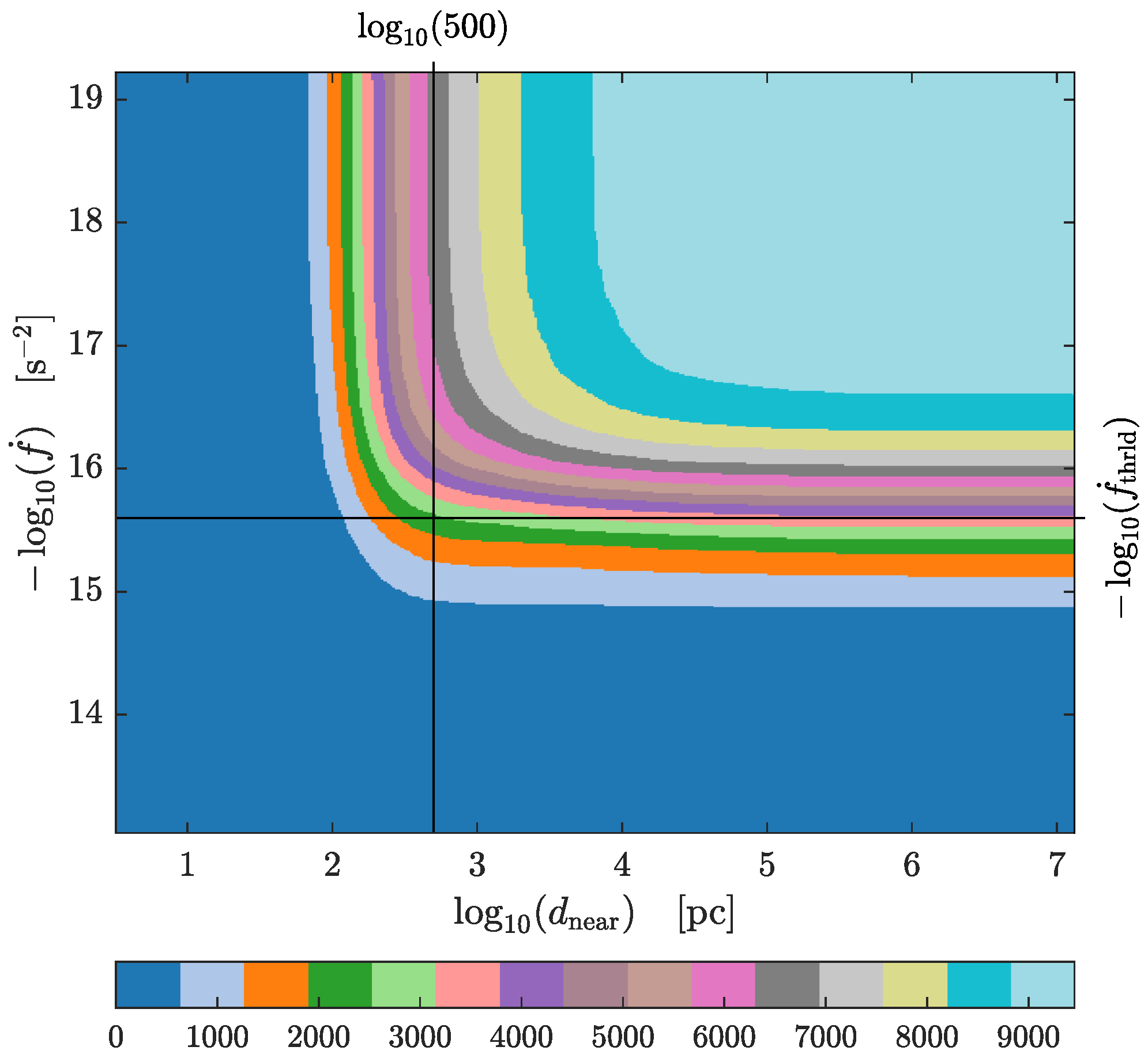
3.1. Distance Determination and Source Selection Methodology

For binary systems undergoing orbital decay exclusively through GW radiation ($\dot{f}>0$), the luminosity distance $\left(d_L\right)$ can be analytically derived by relating observable parameters: frequency (f), frequency derivative ($\dot{f}$), and gravitational wave amplitude ($\mathcal{A}$). This relationship is expressed as:

$$d_L={\displaystyle \frac{5c\dot{f}}{48{\pi }^2{f}^3\mathcal{A}}}.$$

(6)

The spatial distribution reconstruction of galactic binaries critically depends on the precision of these three parameters. While frequency and amplitude measurements achieve high precision, $\Delta f/f\sim {10}^{-5}$ and $\Delta \mathcal{A}/\mathcal{A}\sim {10}^{-2}$$\Delta \mathcal{A}/\mathcal{A}\sim {10}^0$ for SNR $>10$, where $\Delta$ means the difference of estimated parameter and corresponding true parameters. Frequency derivative estimation presents significant challenges. For slowly evolving binaries, which constitute the majority of the galactic population, the frequency evolution requires extended observation periods to measure accurately.

The frequency derivative resolution limit scales as $1/T_{\mathrm{obs}}^2$, yielding approximately $2.5138\times {10}^{-16}{\mathrm{s}}^{-2}$ for our 2-year observation period. Analysis of GBSIEVER output reveals numerous sources with estimated $\dot{f}$ values clustering near this limit, while their true values are 2 to 3 orders of magnitude smaller. This systematic overestimation would significantly distort distance calculations via Equation (6), artificially placing these sources at much greater distances than their true positions.

To mitigate these measurement biases and obtain an accurate representation of the galactic binary population, we implement a two-tiered selection methodology. First, we establish a frequency derivative threshold at ${\dot{f}}_{\mathrm{thrld}}=2.5138\times {10}^{-16}$ $s^{-2}$, corresponding to the theoretical resolution limit, and reject all reported sources with $\dot{f}<{\dot{f}}_{\mathrm{thrld}}$. This criterion eliminates sources with potentially overestimated frequency derivatives that would yield unreliable distance measurements. Second, as the frequency derivative criterion alone proves insufficient, we introduce a proximity criterion that identifies and excludes isolated outliers. We implement a nearest-neighbor distance threshold of $d_{\mathrm{near}}=500$ pc, retaining only sources with at least one neighboring source within this radius. This approach exploits the expected spatial clustering of genuine astrophysical sources, effectively filtering out spurious detections that typically appear as isolated points. The threshold value was optimized through iterative testing to balance outlier elimination against preservation of genuine sources in lower-density regions.

Figure 1 shows the effect of the two selection cuts above. We see that the cuts yield a more coherent and physically plausible distribution of sources with appropriate concentration toward the galactic plane and bulge. By applying these combined selection criteria, we identify approximately 2100 high-quality reported sources that are then used for estimating the galactic structure parameters.

Our selection cut thresholds are justified using a more thorough study. Figure 2 illustrates the cumulative number of reported sources that remain as a function of the two thresholds, ${\dot{f}}_0$ and $d_{\mathrm{near},0}$, with color intensity representing reported source counts satisfying $\dot{f}>{\dot{f}}_0$ and $d_{\mathrm{near}}<d_{\mathrm{near},0}$. The cumulative source count exhibits characteristic behavior across the parameter space, with notably sparse populations in regions of restrictive selection criteria. Specifically, low source counts occur in areas with small proximity thresholds, high frequency derivative thresholds, and particularly in their intersection region (lower-left quadrant of the parameter space). The source count increases systematically as the frequency derivative threshold decreases and the proximity threshold increases, reflecting the trade-off between selection stringency and sample size. However, optimal source selection requires balancing statistical completeness with quality constraints. The two black lines in Figure 2 delineate our chosen thresholds (${\dot{f}}_0$ and $d_{\mathrm{near},0}$), positioned to capture a substantial population while maintaining sufficient selectivity. This threshold combination ensures a robust subset of sources that satisfies both the sensitivity requirements of our analysis and the quality standards necessary for reliable astrophysical interpretation.

While our approach necessarily excludes some genuine sources, the primary objective is to ensure the fidelity of the reconstructed galactic structure rather than catalog completeness. Future work with extended observation periods would naturally improve the precision of $\dot{f}$ measurements, allowing for the inclusion of a larger fraction of the detected population and potential refinement of these selection criteria.

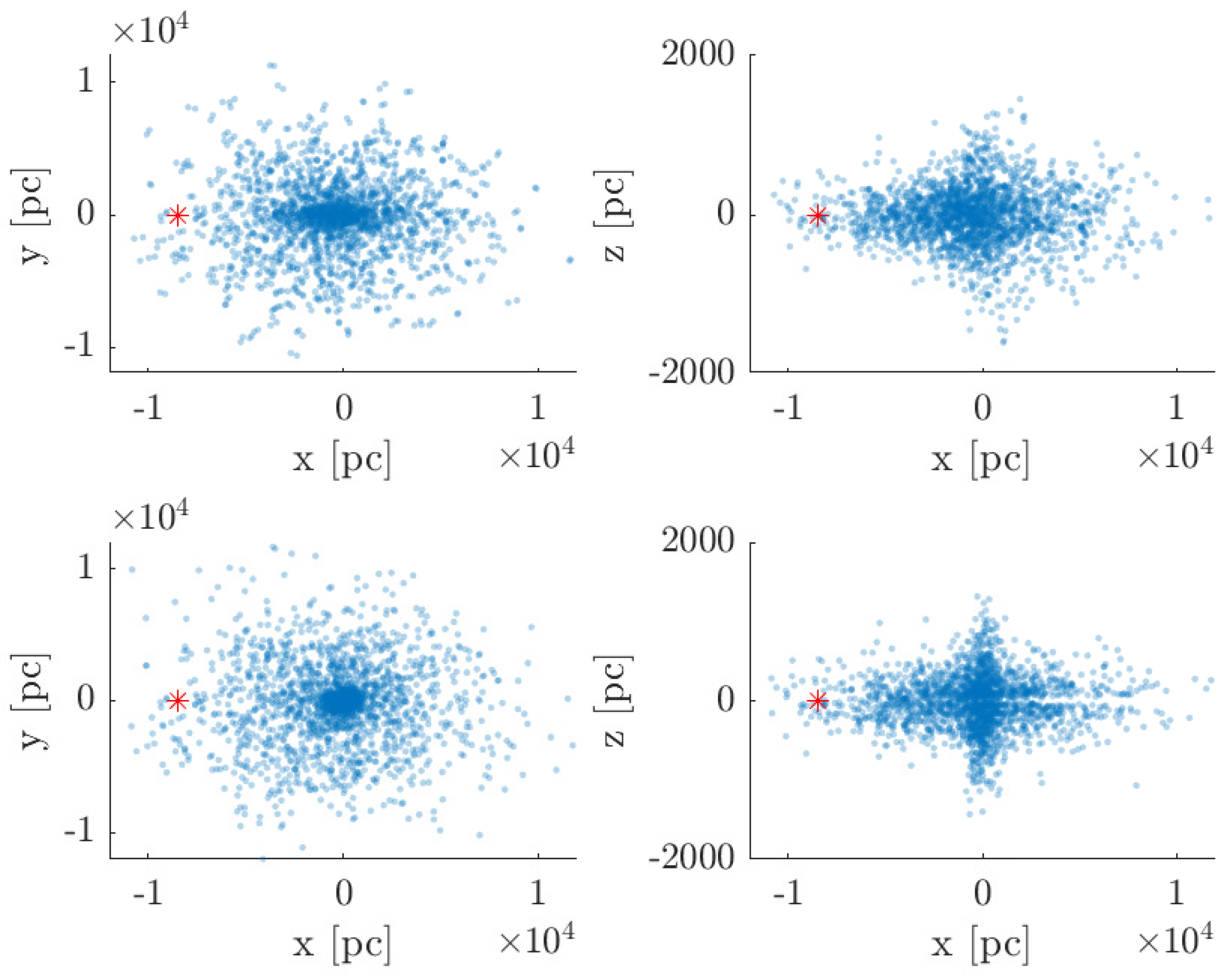
3.2. Galactic Spatial Distribution Model

For characterizing the three-dimensional distribution of GB systems, we adopt a standard composite bulge-disk configuration following [24]. We select this model for its low dimensionality while remaining adequate to describe the essential features of the Milky Way, making it suitable for an initial analysis using gravitational wave observations. This physically motivated framework incorporates the primary structural components of spiral galaxies by accounting for both the bulge and thin disc components. Future investigations can explore higher-dimensional models that may incorporate additional components such as a bar structure instead of a spherical bulge, thick disc, and dark matter halo. The spatial density distribution $\rho (x,y,z)$ of our simple two-component galaxy model is expressed as:

$${\displaystyle \frac{\rho (x,y,z)}{{\rho }_0}}=A{e}^{-r^2/R_b^2}+(1-A)e^{-u/R_d}{\mathrm{sech}}^2(z/Z_d),$$

(7)

where ${\rho }_0$ is the reference density of stars, $r=\sqrt{x^2+y^2+z^2}$ represents the spherical radial distance from the Galactic Center, while $u=\sqrt{x^2+y^2}$ denotes the cylindrical radial distance in the galactic plane. The parameter $R_b$ characterizes the scale radius of the bulge component, which is modeled as a spherically symmetric Gaussian distribution. The disk component is parameterized by a radial scale length $R_d$ and a vertical scale height $Z_d$, with the vertical structure following a hyperbolic secant-squared profile that naturally arises from isothermal disk models in equilibrium under their own self-gravity. The parameter $A\in [0,1]$ determines the relative contribution of the bulge component to the overall density distribution.

The model parameters ${\mathit{\theta }}_{\mathrm{gal}}$$=\{R_b,R_d,Z_d,A,x_{\odot },y_{\odot },z_{\odot }\}$ constitute the primary targets of our inference procedure, where $x_{\odot }, y_{\odot }$ and $z_{\odot }$ represent the Cartesian coordinates of the Solar System within the Milky Way. To align with common practice, we define $R_{\odot }=\sqrt{x_{\odot }^2+y_{\odot }^2}$ in Section 4. The inclusion of these solar position parameters allows us to simultaneously constrain both the intrinsic galactic structure and our location within it, taking advantage of the all-sky coverage provided by gravitational wave observations.

A critical aspect of implementing this model involves the appropriate coordinate transformations between different reference frames. The spatial positions of our sources are initially estimated in terms of luminosity distance $d_L$ and sky position angles $(\lambda ,\beta )$ in the Solar System Barycentric (SSB) reference frame, which is based on the ecliptic coordinate system. However, our galactic structure model is naturally expressed in galactic coordinates, with the origin at the Galactic Center and the primary plane aligned with the galactic disk.

To bridge these different coordinate systems, we implement a three-stage transformation process. First, we convert the ecliptic coordinates $(\lambda ,\beta )$ to declination $\left(\delta \right)$ and right ascension $\left(\alpha \right)$ using the standard astronomical transformation:

$$\begin{array}{cc}\hfill sin\delta & =sinϵcos\beta sin\lambda +cosϵsin\beta ,\hfill \end{array}$$

(8)

$$\begin{array}{cc}\hfill tan\alpha & ={\displaystyle \frac{cosϵcos\beta sin\lambda -sinϵsin\beta }{cos\beta cos\lambda }},\hfill \end{array}$$

(9)

where $ϵ\approx 23.4^{\circ }$ is the obliquity of the ecliptic, representing the tilt angle between the Earth equatorial plane and the ecliptic plane.

In the second stage, we transform from equatorial coordinates $(\alpha ,\delta )$ to galactic longitude $\left(l\right)$ and galactic latitude $\left(b\right)$ following

$$\begin{array}{cc}\hfill sinb& =sin\delta sin{\delta }_N+cos\delta cos{\delta }_{N}cos(\alpha -{\alpha }_N),\hfill \end{array}$$

(10)

$$\begin{array}{cc}\hfill tan(l-l_0)& ={\displaystyle \frac{cos\delta sin(\alpha -{\alpha }_N)}{cos{\delta }_{N}sin\delta -sin{\delta }_{N}cos\delta cos(\alpha -{\alpha }_N)}},\hfill \end{array}$$

(11)

where $({\alpha }_N,{\delta }_N)\approx (192.{85}^{\circ },27.{13}^{\circ })$ are the equatorial coordinates of the North Galactic Pole, and $l_0\approx 122.{93}^{\circ }$ is the galactic longitude of the equatorial North Pole [25].

These two transformations provide us with the galactic longitude and latitude $(l,b)$ of each source. Combined with the luminosity distance $d_L$, we now have the position of each source in a galactic coordinate system still centered on the Solar System.

The final stage translates this Solar-centered galactic coordinate system to the Galactic Center. We convert from the galactic spherical coordinates $(l,b,d_L)$ to galactic Cartesian coordinates $(x,y,z)$ centered on the Galactic Center:

$$\begin{array}{cc}\hfill x& =d_{L}cosbcosl-x_{\odot },\hfill \end{array}$$

(12)

$$\begin{array}{cc}\hfill y& =d_{L}cosbsinl-y_{\odot },\hfill \end{array}$$

(13)

$$\begin{array}{cc}\hfill z& =d_{L}sinb-z_{\odot }.\hfill \end{array}$$

(14)

We search the location of the solar system in the galactic frame in the Cartesian coordinates $(x_{\odot },y_{\odot },z_{\odot })$, then we calculate the cylindrical radial distance $R_{\odot }$. The parameter $z_{\odot }$ quantifies the Sun height above or below the galactic plane. Contemporary astronomical measurements from various methods, including stellar kinematics and astrometry, place the Sun at $R_{\odot }\approx 8.0$ to $8.5$ kpc and $z_{\odot }\approx 20$ to 30 pc [26,27]. However, recognizing that these values remain subject to ongoing refinement, we incorporate both $R_{\odot }$ and $z_{\odot }$ as free parameters in our galactic structure model, allowing the gravitational wave data itself to provide independent constraints on the location of Solar System.

These galactic Cartesian coordinates $(x,y,z)$ centered on the Galactic Center are then directly used in our density model $\rho (x,y,z)$ to evaluate the likelihood function. By properly accounting for these coordinate transformations, we ensure that our inference procedure correctly maps the observed source positions to the underlying galactic structure model, allowing for robust estimation of the structural parameters ${\mathit{\theta }}_{\mathrm{gal}}$.

3.3. Maximum Likelihood Estimation

To quantitatively constrain the structural parameters of the galactic population structure based on our selected GBSIEVER reported sources, we employ a Maximum Likelihood Estimator approach. This statistical framework allows us to infer population-level parameters from the spatial distribution of observed sources while accounting for observational uncertainties and selection effects. The likelihood function for the model parameters ${\mathit{\theta }}_{\mathrm{gal}}$, given our observed data $\widehat{\mathit{x}}$, is formulated as

$$\mathcal{L}({\mathit{\theta }}_{\mathrm{gal}};\widehat{\mathit{x}})=\prod _i{\mathcal{L}}_i({\widehat{\mathit{x}}}_i;{\mathit{\theta }}_{\mathrm{gal}}),$$

(15)

where i represents the index of individual GBSIEVER reported sources that have passed our selection criteria. The Maximum Likelihood Estimator ${\widehat{\mathit{\theta }}}_{\mathrm{gal}}$ for the model parameters ${\mathit{\theta }}_{\mathrm{gal}}$ is given by

$${\widehat{\mathit{\theta }}}_{\mathrm{gal}}=\underset{{\mathit{\theta }}_{\mathrm{gal}}\in \Theta }{arg\; max}\mathcal{L}({\mathit{\theta }}_{\mathrm{gal}};\widehat{\mathit{x}}).$$

(16)

For computational convenience, we work with the logarithm of the likelihood function:

$$ln\mathcal{L}({\mathit{\theta }}_{\mathrm{gal}};\widehat{\mathit{x}})=\sum _{i}ln{\mathcal{L}}_i({\widehat{\mathit{x}}}_i;{\mathit{\theta }}_{\mathrm{gal}}).$$

(17)

This transformation preserves the location of the maximum while avoiding numerical underflow issues that can arise when multiplying many small probabilities.

The individual likelihood contribution from the i-th source ${\mathcal{L}}_i$ is given by:

$${\mathcal{L}}_i({\widehat{\mathit{x}}}_i;{\mathit{\theta }}_{\mathrm{gal}})=\int P\left({\widehat{\mathit{x}}}_i\right|\mathit{x})P_{\mathrm{Gal}}\left(\mathit{x}\right|{\mathit{\theta }}_{\mathrm{gal}})\mathrm{d}\mathit{x},$$

(18)

where $P\left({\widehat{\mathit{x}}}_i\right|\mathit{x})$ is the probability of observing a source at location $\widehat{\mathit{x}}$ given its true spatial position $\mathit{x}$ and accounts for the estimation errors in GB source resolution, including positional errors arising from the calculation of the luminosity distance. The term $P_{\mathrm{Gal}}\left(\mathit{x}\right|{\mathit{\theta }}_{\mathrm{gal}})$ represents the probability density function of the true spatial position $\mathit{x}$ given our model parameters ${\mathit{\theta }}_{\mathrm{gal}}$. In our case, $P_{\mathrm{Gal}}\left(\mathit{x}\right|{\mathit{\theta }}_{\mathrm{gal}})$ is equal to the galactic structure model described in Equation (7).

A comprehensive treatment of the measurement error model, $P\left({\widehat{\mathit{x}}}_i\right|\mathit{x})$ would involve the propagation of uncertainties from the primary observables (f, $\dot{f}$, and $\mathcal{A}$) to the derived spatial coordinates. This is very challenging in the case of GB resolution given the complex correlations and non-linearities arising from the presence of multiple sources along with unresolved ones. Even for simple approaches, such as an FIM analysis of errors for individual sources, it cannot adequately address issues such as the degeneracy of $d_L$ with respect to f, $\dot{f}$, and $\mathcal{A}$, particularly for sources with low signal-to-noise ratios or those near the detection threshold.

In the present paper, we choose to consider a simpler approach to establish baseline performance levels for our overall approach and assume $P\left({\widehat{\mathit{x}}}_i\right|\mathit{x})$ to be a Dirac-delta function,

$$P\left({\widehat{\mathit{x}}}_i\right|\mathit{x})=\delta ({\widehat{\mathit{x}}}_i-\mathit{x}),$$

(19)

effectively assuming that the observed positions are precise measurements of the true positions for sources that have passed our selection criteria. This simplification serves as the first step in the development of a more mature method in future work where the challenges outlined above in constructing $P\left({\widehat{\mathit{x}}}_i\right|\mathit{x})$ shall be investigated systematically. However, as discussed later, we do not stop in this paper at Equation (19) but take a step beyond by doing a statistical analysis that provides some guidance regarding the performance loss and bias it entails.

Given the complex likelihood surface characterized by Equations (17) and (18) in high-dimensional parameter space $\Theta$, traditional gradient-based optimization methods may converge to local maxima rather than the global maximum of interest. To mitigate this risk and efficiently explore the parameter space, we implement PSO algorithm for the likelihood maximization. PSO is a population-based stochastic optimization technique inspired by social behavior of bird flocking or fish schooling, which maintains a swarm of candidate solutions (particles) that move through the parameter space according to simple mathematical formulae combining the current best known positions of individual particles and the swarm as a whole.

In our implementation, we initialize a swarm of 40 particles randomly distributed across the parameter space, with positions constrained to ranges for each parameter: $R_b\in [0,50,000]$ pc, $R_d\in [0,100,000]$ pc, $Z_d\in$ [0, 50,000] pc, $A\in [0,1]$, $(x_{\odot },y_{\odot })\in$ [−500,000, 50,0000] pc, and $z_{\odot }\in$ [−5000, 5000] pc. Since we model source locations using Dirac-delta functions, we deliberately set search ranges approximately ∼100 times larger than the true values (except for the bulge contribution parameter). In future work, when implementing more realistic probability density functions for position estimation errors, these ranges could be adjusted to values more closely aligned with the relevant integration region.

In the PSO algorithm, each particle is characterized by two fundamental attributes: its position, which represents the particle’s current location in the solution space and encodes a candidate solution to the optimization problem, and its velocity, which determines the magnitude and direction of the particle’s movement through the search space. The particles are updated iteratively according to:

$$\begin{array}{cc}\hfill {\mathit{v}}_j^{\left(i\right)}[t+1]=& w{\mathit{v}}_j^{\left(i\right)}\left[t\right]+c_1{\mathit{R}}_1({\mathit{p}}_j^{\left(i\right)}\left[t\right]-{\mathit{r}}_j^{\left(i\right)}\left[t\right])+c_2{\mathit{R}}_2({\mathit{g}}_j\left[t\right]-{\mathit{r}}_j^{\left(i\right)}\left[t\right])\hfill \end{array}$$

(20)

$$\begin{array}{cc}\hfill {\mathit{r}}_j^{\left(i\right)}[t+1]=& {\mathit{r}}_j^{\left(i\right)}\left[t\right]+{\mathit{v}}_j^{\left(i\right)}[t+1]\hfill \end{array}$$

(21)

where t denotes the iteration number, j denotes the search space dimension index and $\left(i\right)$ represents the index of a particle. ${\mathit{r}}_j^{\left(i\right)}\left[t\right]$ and ${\mathit{v}}_j^{\left(i\right)}\left[t\right]$ are the position and velocity particle i at iteration t, ${\mathit{p}}_j^{\left(i\right)}$ is the best position found by particle i so far, ${\mathit{g}}_j$ is the best position found by any particle in the swarm, w is the inertia weight, $c_1$ and $c_2$ are acceleration coefficients, and ${\mathit{R}}_1$ and ${\mathit{R}}_2$ are random numbers drawn from a uniform distribution in $[0,1]$.

The PSO algorithm is particularly well-suited for our application due to its ability to handle non-differentiable objective functions, its robustness against local maxima, and its efficient parallel implementation. We run the algorithm for a maximum of 2000 iterations. To improve the robustness of our results, we perform 6 independent runs with different random initializations and pick the best resulting optimal parameter values.

4. Results

In this section we show our main results for this work.

4.1. Galactic Structure Parameter Estimation

We applied our maximum likelihood analysis to two distinct datasets: (i) the true sources from the LDC GB catalog, representing an idealized scenario with perfect source detection, and (ii) the reported sources from our GBSIEVER algorithm after applying the two-tiered selection methodology described in Section 3.1. This comparative approach allows us to assess the robustness of our parameter estimation procedure under realistic observational constraints.

Figure 3 compares the spatial distributions derived from true catalog sources and GBSIEVER-reported sources after the selection cuts are applied. The post-selection cut set of reported sources are then used for the estimation of the galactic structure parameters using the formalism described in Section 3.3. Both distributions show a concentration toward the Galactic Center and a flattened disk structure typical of spiral galaxies like the Milky Way. The reported sources display a somewhat less compact and more elliptical center distribution in the $\mathrm{x}\text{-}\mathrm{y}$ plane. The vertical structure shown in the $\mathrm{x}\text{-}\mathrm{z}$ projections shares some similarities between the two datasets, which aligns with our comparable disk scale height estimates. While the general galactic structure is recognizable in our reconstruction, noticeable differences in the density distribution reflect the inherent limitations when working with reported rather than true source positions.

Examination of the spatial distribution of GB systems in the LDC catalog reveals a notable gap around $z\approx 0$ around the galactic plane. This feature likely arises from the simulation incorporation of realistic observational biases present in electromagnetic surveys, which struggle to detect objects at low galactic latitudes ($\left|b\right|<10$) due to dust extinction and stellar crowding [28]. By including these observational constraints, the LDC provides an authentic representation of the GB population. Future gravitational wave observations with spaceborne GW observatory like LISA will transcend these limitations, as gravitational waves propagate unaffected by intervening matter. This advantage underscores one of the fundamental strengths of gravitational wave astronomy: its capacity to deliver an unobscured view of source distributions throughout the Galaxy, including regions largely inaccessible to conventional electromagnetic observations.

Table 2. Maximum likelihood estimates for the galactic structure parameters derived from GBSIEVER after applying our selection criteria. These values correspond to the global maximum of the likelihood function determined by the PSO algorithm.

Parameter	Description	Recovered Value
$R_b$	Bulge scale radius	$916.07\mathrm{pc}$
$R_d$	Disk scale length	$1976.02\mathrm{pc}$
$Z_d$	Disk scale height	$346.25\mathrm{pc}$
A	Bulge fraction	$0.13$
$R_{\odot }$	Solar distance from Galactic Center	$8.15\mathrm{kpc}$
$z_{\odot }$	Solar height above galactic plane	$-804.30\mathrm{pc}$

presents the results of galactic model parameters obtained from selected GBSIEVER reported sources using the PSO algorithm. The literature provides reference values for these galactic structure parameters based on various observational techniques. For the bulge component, previous studies suggest a scale radius $R_b$ of approximately 500 pc, smaller than our estimate of 916.07 pc. The typical bulge fraction A in galactic models is around 0.25, while our lower value is 0.13. The disk scale length $R_d$ has been estimated at approximately 2500 pc from stellar surveys, somewhat larger than our value of 1976.02 pc. For the vertical structure, the canonical thin disk scale height $Z_d$ is approximately 300 pc, while our estimate of 346.25 pc. Regarding the position of the Solar System, determinations place the Sun at a distance of approximately 8.0 to 8.5 kpc from the Galactic Center $R_{\odot }$ [26], which is reasonably consistent with our estimate of 8.15 kpc. However, the Solar height above the galactic plane $z_{\odot }$ is typically measured at approximately −30 pc [27], considerably different from our estimate of −804.30 pc. This notable discrepancy in $z_{\odot }$ may reflect systematic biases in the LDC GB population model, limitations in our distance estimation methodology, or selection effects in our sample of GB systems—all possibilities that warrant further investigation in future work.

It is important to note that the true parameter values used by the LDC to generate the simulated galactic binary population remain undisclosed to analysts. This blind analysis approach deliberately mirrors real observational scenarios and enables an unbiased assessment of parameter recovery techniques, though it limits our ability to directly evaluate the accuracy of our estimates against the simulation’s ground truth values.

4.2. Effect of Measurement Errors

To evaluate the impact of the simplified model of measurement uncertainties given in Equation (19), we conducted the experiment described below using the true source catalog. First, we established a threshold of ${\mathrm{SNR}}_{\mathrm{low}}\approx 10$, derived from the lowest signal-to-noise ratio observed in our reported sources, and randomly selected 100 subsets of true LDC catalog sources. Each subset had approximately 2100 sources with positive frequency derivatives ($\dot{f}>0$) and $\mathrm{SNR}>{\mathrm{SNR}}_{\mathrm{low}}$, corresponding to the number of reported sources meeting our two-tiered selection criteria. For these true sources, we implemented less stringent constraints on $\dot{f}$, as they are not subject to the systematic errors inherent in detected sources. The Maximum Likelihood Estimation procedure using the measurement error model in Equation (19) was applied to each subset, generating the corresponding number of estimates for ${\mathit{\theta }}_{\mathrm{gal}}$.

It is important to note that when applied to true sources, Equation (19) represents the exact measurement uncertainty model rather than an approximation. The purpose of this experiment is not to obtain the most accurate galactic parameter estimates, but rather to isolate and quantify the systematic effects introduced by our specific measurement uncertainty assumptions in Equation (19). By using true sources, we can separate the impact of our modeling choices from other sources of error, thereby providing insight into how these assumptions influence the parameter estimation process independent of detection-related biases.

Figure 4 presents the distribution of normalized parameter estimates ${\tilde{\mathit{\theta }}}_{\mathrm{gal};i,j}=({\widehat{\mathit{\theta }}}_{\mathrm{gal};i,j}-{\mu }_j)/{\sigma }_j$ compared against the results from Table 2. Here, ${\widehat{\mathit{\theta }}}_{\mathrm{gal};i,j}$ represents the j-th parameter value from the i-th subset, and ${\tilde{\mathit{\theta }}}_{\mathrm{gal};i,j}$ is the normalized parameter values. ${\mu }_j$ and ${\sigma }_j$ denote the mean value and standard deviation, respectively, of the j-th parameter calculated across all 100 subsets. We see varying degrees of agreement between our results and the true-source distributions.

For the location of the solar system, our reported-source estimates fall near the center of the true-source distributions, while the structure of the Milky Way shows more notable offsets. Interestingly, the estimated $z_{\odot }$ shows a consistent deviation from the literature value of approximately $-30$ pc across trials. This discrepancy may arise partly from limitations in the model or simulation used for generating the LDC catalog or our use of subsets of true sources. The scale sizes of the bulge and disk derived from reported sources differ considerably from the statistical distribution of results obtained from true sources. These discrepancies may be attributed to the systematic differences in spatial distribution observed between reported and true LDC catalog sources, where true sources exhibit significantly higher central concentration and a more spherical distribution compared to the more extended and more elliptical distribution of reported sources, as illustrated in our earlier comparison in Figure 3.

Despite the above limitations arising from Equation (19), the estimated parameter values from reported sources remain within astronomically reasonable ranges. This indicates that although our methodology may not yet achieve optimal precision in parameter recovery, it constrains galactic structural parameters to physically plausible values. These results support the fundamental promise of our approach for recovering structural features of the Galaxy, though future significant refinement of our methodology will be necessary to improve agreement with true source distributions before drawing definitive astrophysical conclusions.

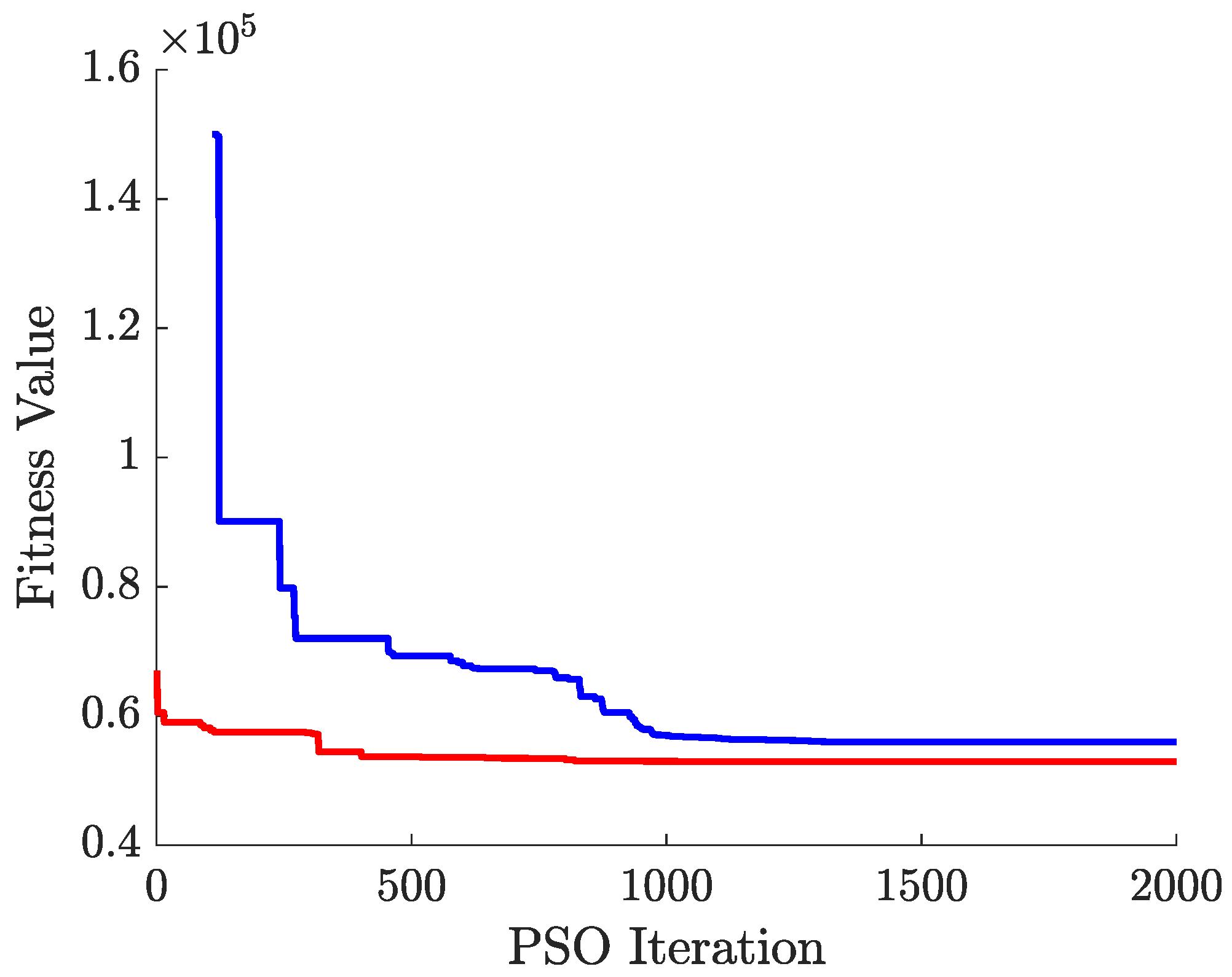
4.3. PSO Algorithm Performance

The PSO algorithm proved effective in navigating the complex likelihood surface associated with our parameter estimation problem. Figure 5 illustrates the convergence behavior of the algorithm for both datasets.

The algorithm typically converged within ∼1000 iterations, with the likelihood function stabilizing thereafter. The consistent convergence behavior across multiple independent runs with different initial conditions supports the robustness of our parameter estimates and suggests that the algorithm successfully located the global maximum of the likelihood function rather than becoming trapped in local maxima.

5. Conclusions

In this work, we have taken the first steps towards evaluating the capability of GW observations using LISA or other equivalent spaceborne detectors to estimate the galactic structure when parameter estimation errors are included. The gravitational wave approach offers unique advantages through its immunity to dust extinction and its sensitivity to old stellar populations throughout the Galaxy, including regions that remain largely inaccessible to electromagnetic surveys. This capability will be particularly valuable for studying the central regions and the mid-plane of the Galaxy, where dust obscuration presents significant challenges for conventional observations. Our results support the promise of spaceborne GW observatories like LISA serving as a new probe of galactic structure, complementary to traditional electromagnetic observations, but also outline the challenges involved once realistic data analysis is taken into account.

Our analysis pipeline combines the GBSIEVER algorithm for source detection with a maximum likelihood approach for galactic structure parameter estimation. While we have presented the complete mathematical formalism, a major simplification was made in this initial study, where the probability of estimated parameters conditioned on true ones is approximated as a Dirac delta function. The method was applied to LDC data and despite the approximation, the method was able to recover structural parameters of the Milky Way bulge and disk components in the ballpark of widely adopted values. We consider this to be a promising result, given that ours is the first attempt to include realistic parameter estimation errors. To test the effect of the above approximation, the same method was applied to subsets of the true catalog of GBs used for generating the LDC data. The latter does not guarantee recovery of the true galactic structural parameters used for constructing the catalog. (In fact, there is an anomaly in the height of the Solar System of the galactic plane even with the true catalog.) Nonetheless, this experiment points out that the approximation will need to be replaced in future improvements to the method.

A key step necessary in extracting useful results from the reported catalog of GBs is the two-tiered selection procedure we developed—combining frequency derivative thresholding and proximity criteria. This step was necessitated by the systematic overestimation of frequency derivatives for slowly evolving binaries, which would otherwise lead to severely distorted distance measurements and unreliable galactic structure inference. Our analysis demonstrates that without these selection criteria, the spatial distribution of sources fails to reveal the underlying galactic structure, highlighting the importance of source selection in our specific methodology that reconstructs the galactic structure under realistic conditions.

In future work, we plan to remedy the deficiencies and challenges discovered in this work. A key improvement will involve incorporating realistic error distributions from GBSIEVER parameter estimation process rather than using an over-simplified delta function assumption. This more comprehensive treatment of uncertainties will enable us to relax our currently stringent two-tiered selection criteria while maintaining reliable galactic structure recovery. With an improved method, we also intend to explore more complex galactic models incorporating non-axisymmetric features such as spiral arms and the galactic bar, potentially revealing subtler structural components from gravitational wave observations. Additional refinements will include improved handling of the confusion noise background and investigation of how different binary evolution models affect the inferred galactic parameters.

An important avenue for future work involves combining our current $\mathcal{F}$-statistic-based approach with global fit methodologies, which would better handle parameter degeneracies and provide more accurate uncertainty estimates, particularly for distance measurements where amplitude and inclination estimation errors significantly impact precision. We also recognize that other datasets of simulated galactic binaries, such as LDC2a and Taiji Data Challenge 2, represent valuable opportunities for galactic structure parameter estimation studies and would provide important additional validation of our methodology across different data challenge scenarios. Also, a network of space-based detectors and longer observation times are expected to improve the accuracy of estimated GB parameters, with corresponding benefits to the reconstruction of the galaxy using the reported sources.

References

1. Amaro-Seoane, P.; Audley, H.; Babak, S.; Baker, J.; Barausse, E.; Bender, P.; Berti, E.; Binetruy, P.; Born, M.; Bortoluzzi, D.; et al. Laser Interferometer Space Antenna. arXiv 2017, arXiv:1702.00786. [Google Scholar]
2. Siebenmorgen, R.; Voshchinnikov, N.; Bagnulo, S. Dust in the diffuse interstellar medium-Extinction, emission, linear and circular polarisation. Astron. Astrophys. 2014, 561, A82. [Google Scholar] [CrossRef]
3. Gontcharov, G. Interstellar extinction. Astrophysics 2016, 59, 548–579. [Google Scholar] [CrossRef]
4. Littenberg, T.B. Detection pipeline for Galactic binaries in LISA data. Phys. Rev. D—Part Fields, Gravit. Cosmol. 2011, 84, 063009. [Google Scholar] [CrossRef]
5. Babak, S.; Baker, J.G.; Benacquista, M.J.; Cornish, N.J.; Larson, S.L.; Mandel, I.; McWilliams, S.T.; Petiteau, A.; Porter, E.K.; Robinson, E.L.; et al. The mock LISA data challenges: From challenge 3 to challenge 4. Class. Quantum Gravity 2010, 27, 084009. [Google Scholar] [CrossRef]
6. Korol, V.; Rossi, E.M.; Barausse, E. A multimessenger study of the Milky Way’s stellar disc and bulge with LISA, Gaia, and LSST. Mon. Not. R. Astron. Soc. 2019, 483, 5518–5533. [Google Scholar] [CrossRef]
7. Korol, V.; Toonen, S.; Klein, A.; Belokurov, V.; Vincenzo, F.; Buscicchio, R.; Gerosa, D.; Moore, C.; Roebber, E.; Rossi, E.; et al. Populations of double white dwarfs in Milky Way satellites and their detectability with LISA. Astron. Astrophys. 2020, 638, A153. [Google Scholar] [CrossRef]
8. Wilhelm, M.J.; Korol, V.; Rossi, E.M.; D’Onghia, E. The Milky Way’s bar structural properties from gravitational waves. Mon. Not. R. Astron. Soc. 2021, 500, 4958–4971. [Google Scholar] [CrossRef]
9. Kay, S.M. Fundamentals of Statistical Signal Processing: Estimation Theory; Prentice-Hall, Inc.: Upper Saddle River, NJ, USA, 1993. [Google Scholar]
10. Balasubramanian, R.; Sathyaprakash, B.S.; Dhurandhar, S. Gravitational waves from coalescing binaries: Detection strategies and Monte Carlo estimation of parameters. Phys. Rev. D 1996, 53, 3033. [Google Scholar] [CrossRef]
11. Babak, S.; Petiteau, A. LISA Data Challenge Manual; Technical Report LISA-LCST-SGS-MAN-002; APC: Paris, France, 2020; Available online: https://sbgvm-151-90.in2p3.fr/static/data/pdf/LDC-manual-002.pdf (accessed on 20 July 2025).
12. Breivik, K.; Mingarelli, C.M.; Larson, S.L. Constraining galactic structure with the LISA white dwarf foreground. Astrophys. J. 2020, 901, 4. [Google Scholar] [CrossRef]
13. Georgousi, M.; Karnesis, N.; Korol, V.; Pieroni, M.; Stergioulas, N. Gravitational waves from double white dwarfs as probes of the milky way. Mon. Not. R. Astron. Soc. 2023, 519, 2552–2566. [Google Scholar] [CrossRef]
14. Zhang, S.; Deng, F.; Lu, Y.; Yu, S. Constraining the Galactic Structure Using Time Domain Gravitational Wave Signal from Double White Dwarfs Detected by Space Gravitational Wave Detectors. Astrophys. J. 2024, 978, 61. [Google Scholar] [CrossRef]
15. Ruan, W.H.; Guo, Z.K.; Cai, R.G.; Zhang, Y.Z. Taiji program: Gravitational-wave sources. Int. J. Mod. Phys. A 2020, 35, 2050075. [Google Scholar] [CrossRef]
16. Karnesis, N.; Babak, S.; Pieroni, M.; Cornish, N.; Littenberg, T. Characterization of the stochastic signal originating from compact binary populations as measured by LISA. Phys. Rev. D 2021, 104, 043019. [Google Scholar] [CrossRef]
17. Zhang, X.H.; Mohanty, S.D.; Zou, X.B.; Liu, Y.X. Resolving Galactic binaries in LISA data using particle swarm optimization and cross-validation. Phys. Rev. D 2021, 104, 024023. [Google Scholar] [CrossRef]
18. Zhang, X.H.; Zhao, S.D.; Mohanty, S.D.; Liu, Y.X. Resolving Galactic binaries using a network of space-borne gravitational wave detectors. Phys. Rev. D 2022, 106, 102004. [Google Scholar] [CrossRef]
19. Baghi, Q. The LISA Data Challenges. arXiv 2022, arXiv:2204.12142. [Google Scholar]
20. Eberhart, R.; Kennedy, J. Particle swarm optimization. In Proceedings of the IEEE International Conference on Neural Networks, Perth, WA, Australia, 27 November–1 December 1995; Volume 4, pp. 1942–1948. [Google Scholar]
21. Jaranowski, P.; Krolak, A.; Schutz, B.F. Data analysis of gravitational—Wave signals from spinning neutron stars. 1. The Signal and its detection. Phys. Rev. D 1998, 58, 063001. [Google Scholar] [CrossRef]
22. Tinto, M.; Dhurandhar, S.V. Time-delay interferometry. Living Rev. Relativ. 2014, 17, 1–54. [Google Scholar] [CrossRef]
23. Donoho, D.L.; Tanner, J. Precise undersampling theorems. Proc. IEEE 2010, 98, 913–924. [Google Scholar] [CrossRef]
24. Adams, M.R.; Cornish, N.J.; Littenberg, T.B. Astrophysical model selection in gravitational wave astronomy. Phys. Rev. D 2012, 86, 124032. [Google Scholar] [CrossRef]
25. Reid, M.J.; Brunthaler, A. The proper motion of Sagittarius A*. II. The mass of Sagittarius A. Astrophys. J. 2004, 616, 872. [Google Scholar] [CrossRef]
26. Reid, M.; Menten, K.; Brunthaler, A.; Zheng, X.; Dame, T.; Xu, Y.; Wu, Y.; Zhang, B.; Sanna, A.; Sato, M.; et al. Trigonometric parallaxes of high mass star forming regions: The structure and kinematics of the Milky Way. Astrophys. J. 2014, 783, 130. [Google Scholar] [CrossRef]
27. Bennett, M.; Bovy, J. Vertical waves in the solar neighbourhood in Gaia DR2. Mon. Not. R. Astron. Soc. 2019, 482, 1417–1425. [Google Scholar] [CrossRef]
28. Tkachenko, R.; Vieira, K.; Lutsenko, A.; Korchagin, V.; Carraro, G. Determining the Scale Length and Height of the Milky Way’s Thick Disc Using RR Lyrae. Universe 2025, 11, 132. [Google Scholar] [CrossRef]
Figure 1. The red stars in the figures denote the location of our solar system in the Milky Way. Effect of distance cut on the shape of reconstructed galaxy. The upper row displays the reconstructed galaxy using reported sources with a proximity threshold of d near = 500 pc applied, while the lower row displays all the reported sources without the threshold. A frequency derivative threshold of 2.5138 × 10 16 s 2 was applied to both reconstructions. Left panels show the face-on view (xy-plane), while right panels show the edge-on view (xz-plane), with the Galactic Center at the origin and the Solar System location marked by the red star.
Universe 11 00248 g001
Figure 2. The number of reported sources left after application of the selection cuts. The two black lines show the thresholds used in our study: d near = 500 pc (vertical) and f ˙ thrld = 2.5138 × 10 16 s 2 (horizontal).
Universe 11 00248 g002
Figure 3. Spatial distribution of selected GBs throughout the Galaxy. Upper panels: results based on reported sources from GBSIEVER after applying our selection criteria. Lower panels: results based on true sources from the LDC catalog.
Universe 11 00248 g003
Figure 4. Distribution of estimated galactic structure parameters from 100 independent trials, each using approximately 2100 randomly selected GBs from the true source catalog. The vertical red lines indicate the values from our analysis of GBSIEVER-reported sources. The distributions are normalized to display deviations of reported source results from the ensemble mean in units of the ensemble standard deviation, providing a statistical comparison between reported sources and true source subsets.
Universe 11 00248 g004
Figure 5. Convergence of the PSO algorithm for maximum likelihood estimation. The plot shows the evolution of the log-likelihood function across iterations for the reported sources (blue) and the LDC catalog sources (red).
Universe 11 00248 g005