Structural Implications of the Chameleon Mechanism on White Dwarfs

Abstract

We study the behaviour of the chameleon mechanism around white dwarfs and its impact on their structure. Using a shooting method of our own design, we solve the corresponding scalar–tensor equilibrium equations for a Chandrasekhar equation of state, exploring various energy scales and couplings of the chameleon field to matter. For the considered parameter ranges, we find the chameleon field to be in a thick-shell configuration, identifying for the first time in the literature a similarity relation of the theory for the radially normalised scalar field gradient. Our analysis reveals that the chameleon mechanism alters the pressure gradient of white dwarfs, leading to a reduction in the stellar radii and masses and shifting the mass–radius curves below those predicted by Newtonian gravity. This also lowers the specific heat of white dwarfs, accelerating their cooling process. Finally, we derive parametric expressions from our results to expedite future analyses of white dwarfs in scalar–tensor theories.

1. Introduction

General Relativity (GR) stands strong as a gravity theory, verified by numerous experiments and observations [1]. Nevertheless, it fails to explain astrophysical and cosmological phenomena like the galactic rotation curves or the fundamental origin of dark energy. This suggests that gravity may not be fully described by GR, but by a modified gravity (MG) theory [2]. A particular class of MG theories is built on adding scalar fields to the tensorial gravitational description of GR. In the so-called scalar–tensor (ST) theories [3,4,5], a scalar field mediates a fifth interaction between matter components. If the range of such a fifth force is long enough, it could potentially contradict the local tests of gravity [1] or enhance structure formation in the early [6,7,8] and late universe [9,10,11,12] (for noteworthy exceptions, see [13,14,15,16]).

However, several ST theories include screening mechanisms that render the scalar field properties environment-dependent. In the chameleon mechanism [17,18,19,20,21], the mass of the scalar field varies with the environment. In the symmetron [22,23,24] and dilaton scenarios [25,26,27], it is the coupling to matter that changes, while, in the Vainshtein [28,29] and k-mouflage implementations [30,31], it is the kinetic function that plays this role. Mechanisms built upon k-essence models [32,33]—extendable to generalised k-essence [34] and quasi-quintessence [35]—also work with the kinetic contribution of the field. The dynamics of the scalar field at astrophysical scales is then different from that at cosmological scales because of these mechanisms.

It has been shown that the characteristics of stellar objects—such as masses, radii, and cooling times—can be affected by the presence of such scalar fields [33,36,37,38,39,40,41,42,43,44,45], for the screening mechanism partially breaks inside compact stars. White dwarfs (WDs) are adequate targets to test such effects, yet they remain comparatively unexplored [46,47,48,49,50]. These stars are particularly suitable for such studies for two main reasons: their internal structure is governed by well-understood equations of state (EoSs) [51], and the Gaia mission has provided high-precision measurements of temperature, luminosity, radius, kinematics, and spatial distribution for over ${10}^5$ WD candidates [52,53,54].

The aim of this paper is to explore the behaviour of the chameleon mechanism around WDs, as well as its effects on their structure. To this end, we numerically integrate the ST equilibrium equations in the relativistic and Newtonian limits employing a Chandrasekhar EoS. By exploring a broad range of energy scales and conformal chameleon coupling to matter, we determine the corresponding mass–radius relations, deriving also a set of ready-to-use fitting formulae aiming to streamline future analyses of WDs in ST theories. In addition, we inspect the impact of the chameleon field on the internal pressure, the specific heat, and the cooling time of these stars.

The structure of the present work is as follows: In Section 2, we discuss the ST framework, the EoS we use to describe WDs, and the equations governing a static and spherically symmetric star in equilibrium Newtonian gravity. In Section 3, we review the chameleon mechanism and the employed numerical methods, with special emphasis on the boundary conditions and our shooting method algorithm. Section 4 contains our results regarding chameleon-screened WDs. We conclude and examine potential extensions of this work in Section 5. Finally, Appendix A provides supplementary details on the validity of the Newtonian approximation in our ST framework. In this paper, unless stated otherwise, we consider the metric signature $(-,+,+,+)$ and $c=\hslash =k_B=1$.

2. Framework

2.1. Scalar–Tensor Theory

The chameleon field theory [17] is an ST theory equipped with a screening mechanism. Like the symmetron, the dilaton, certain $f\left(R\right)$ theories [36], and the low-energy limits of string theories [55], the chameleon is described by the following action:

$$S=\int d^{4}x\sqrt{-g}\left[{\displaystyle \frac{M_P^2}{2}}R-{\displaystyle \frac{1}{2}}{\nabla }_{\mu }\varphi {\nabla }^{\mu }\varphi -V\left(\varphi \right)\right]+S_m\left[{\Psi }_m;A^2\left(\varphi \right)g_{\mu \nu }\right].$$

(1)

Notice that other screening mechanisms, like Vainshtein [28,29] and k-mouflage [30,31], do not fit in the action above because they possess non-canonical kinetic terms. In Equation (1), g is the determinant of the Einstein frame metric $g_{\mu \nu }$, R is the Ricci scalar in that metric, $M_P={\left(8\pi G\right)}^{-1/2}=2.43\times {10}^{18}$ GeV is the reduced Planck mass, and $\varphi$ is the scalar field. Lastly, $V\left(\varphi \right)$ and $A\left(\varphi \right)$ are the self-interacting potential and conformal coupling to matter ${\Psi }_m$, respectively, which characterise the models within this class. Notice that the scalar field couples to matter through the Jordan frame metric ${\tilde{g}}_{\mu \nu }\equiv A^2\left(\varphi \right)g_{\mu \nu }$. This gravitational coupling is the origin of the fifth force between matter fields, which makes these ST theories enter the category of MG theories [38].

By varying Equation (1) with respect to the metric, one obtains the field equations:

$$G_{\mu \nu }={\kappa }^2\left[T_{\mu \nu }+{\nabla }_{\mu }\varphi {\nabla }_{\nu }\varphi -g_{\mu \nu }\left({\displaystyle \frac{1}{2}}{\nabla }_{\sigma }\varphi {\nabla }^{\sigma }\varphi +V\left(\varphi \right)\right)\right],$$

(2)

where $G_{\mu \nu }$ is the Einstein tensor, $\kappa \equiv M_P^{-1}$, and

$$T_{\mu \nu }\equiv -{\displaystyle \frac{2}{\sqrt{-g}}}{\displaystyle \frac{\delta S_m}{\delta g^{\mu \nu }}}$$

(3)

is the matter energy–momentum tensor. Let us assume that matter fields can be described by a perfect fluid, that is,

$$T^{\mu \nu }\equiv (ϵ+P)u^{\mu }{u}^{\nu }+P{g}^{\mu \nu },$$

(4)

with $u^{\mu }$ being the four-velocity, $ϵ$ the total energy density, and P the pressure, all in the rest frame of the fluid. Analogously, if we vary Equation (1) with respect to the field, we obtain the scalar field equation

$$\square \varphi ={\displaystyle \frac{dV\left(\varphi \right)}{d\varphi }}-{\displaystyle \frac{d\ln A\left(\varphi \right)}{d\varphi }}T\equiv {\displaystyle \frac{d{V}_{\mathrm{eff}}\left(\varphi \right)}{d\varphi }},$$

(5)

with $V_{\mathrm{eff}}\left(\varphi \right)$ being the potential effectively governing $\varphi$. Lastly, the hydrostatic equation can be derived from the divergence of Equation (2), namely

$${\nabla }^{\nu }{T}_{\mu \nu }={\displaystyle \frac{d\ln A\left(\varphi \right)}{d\varphi }}T{\nabla }_{\mu }\varphi ,$$

(6)

where $T\equiv g^{\mu \nu }{T}_{\mu \nu }$ is the trace of the energy–momentum tensor. The above equation means that, from the perspective of the Einstein frame, free particles do not follow the $g_{\mu \nu }$ geodesics. This is because they are affected by the fifth force, given by the gradient of the scalar field ${\nabla }_{\mu }\varphi$ through its coupling ${\displaystyle \frac{d\ln A\left(\varphi \right)}{d\varphi }}$. One can also describe this scenario from the perspective of the Jordan frame, defining the corresponding energy–momentum tensor as

$${\tilde{T}}_{\mu \nu }\equiv -{\displaystyle \frac{2}{\sqrt{-\tilde{g}}}}{\displaystyle \frac{\delta S_m}{\delta {\tilde{g}}^{\mu \nu }}}.$$

(7)

Comparing the expressions for the energy–momentum tensor in both frames, Equations (3) and (7), we realise that the relation between them is $T_{\mu \nu }=A^2\left(\varphi \right){\tilde{T}}_{\mu \nu }$. In the Jordan frame, free particles follow ${\tilde{g}}_{\mu \nu }$ geodesics and the energy–momentum tensor is conserved, i.e., ${\tilde{\nabla }}^{\nu }{\tilde{T}}_{\mu \nu }=0$. This means that the fifth force is no longer explicit, as its effect is embedded in the metric. The conformal transformations of the elements in the energy–momentum tensor in both frames come from the relation between both tensors and the normalisation condition for the four-velocity, namely, $g_{\mu \nu }{u}^{\mu }{u}^{\nu }=-1$. The latter expression implies that $u^{\mu }=A\left(\varphi \right){\tilde{u}}^{\mu }$, and yields the following correspondences for total energy density and pressure: $ϵ=A^4\left(\varphi \right)\widetilde{ϵ}$ and $P=A^4\left(\varphi \right)\tilde{P}$.

2.2. Equation of State

The EoS describes how pressure relates to energy density, capturing the microphysical behaviour of matter inside the star. In GR and in the ST theories considered in this work, WDs can be accurately modelled as non-relativistic systems, as we explain here and show in Appendix A. Therefore, it is convenient to decompose the total energy density $\widetilde{ϵ}$ into the rest-mass density $\tilde{\rho }$ and the internal energy density $\tilde{\Pi }$ as follows:

$$\widetilde{ϵ}\equiv \tilde{\rho }\left(1+{\displaystyle \frac{\tilde{\Pi }}{\tilde{\rho }{c}^2}}\right),$$

(8)

where we have explicitly written the speed of light c to evince that $\tilde{\Pi }$ is a relativistic correction of the first order.

Moreover, thermal effects inside WDs can be modelled as fluid dynamics perturbations [51]. Consequently, the EoS depends only on one parameter, namely, $\tilde{P}\left(\tilde{\rho }\right)$, and $\widetilde{ϵ}\left(\tilde{\rho }\right)$. We consider the Jordan frame variables in the EoS because the common thermodynamic energy conservation relation $d(\widetilde{ϵ}/\tilde{\rho })=-\tilde{P}d(1/\tilde{\rho })$ holds in this frame and not in the Einstein one.

The electrostatic energy of matter inside WDs is insignificant against the Fermi energies; hence, the Coulomb forces are as well. Therefore, the electron pressure is given by [51]

$$\tilde{P}={\displaystyle \frac{2}{{\left(2\pi \right)}^3{\hslash }^3}}{\int }_0^{p_{F,e}}{\displaystyle \frac{p^2{c}^2}{\sqrt{p^2{c}^2+{\left(m_e{c}^2\right)}^2}}}4\pi p^{2}dp={\displaystyle \frac{m_e{c}^2}{{\lambda }_e^3}}\psi \left(x\right),$$

(9)

with

$$\psi \left(x\right)={\displaystyle \frac{1}{8{\pi }^2}}\left[x\sqrt{1+x^2}\left({\displaystyle \frac{2x^2}{3}}-1\right)+\ln \left(x+\sqrt{1+x^2}\right)\right],$$

(10)

where, for the sake of clarity, we have made explicit again the different c and ℏ factors. The factor 2 in Equation (9) is due to the spin degeneracy of the electrons. The electron Fermi momentum, mass, and Compton wavelength are denoted by $p_F$, $m_e$, and ${\lambda }_e\equiv \hslash /\left(m_{e}c\right)$, respectively, while $x\equiv p_F/m_{e}c$ is the dimensionless Fermi momentum.

The degenerate electrons are the dominant contributors to pressure $\tilde{P}$ in a WD, while ions account for most of the energy density $\widetilde{ϵ}$. For densities below the neutron drip ${\tilde{\rho }}_{\mathrm{n}\text{-}\mathrm{drip}}\simeq 4\times {10}^{11}\mathrm{g}{\mathrm{cm}}^{-3}$ [51], ions are non-relativistic; hence, $\widetilde{ϵ}$ can be expressed in terms of the rest-mass density:

$$\widetilde{ϵ}=\tilde{\rho }={\displaystyle \frac{m_B{n}_e}{Y_e}}.$$

(11)

where $m_B$ is the mean nucleon mass and $n_e=8\pi p_{F,e}^3/\left(3h^3\right)$ is the electron number density. The mean number of electrons per nucleon is denoted by $Y_e=Z/A$, where Z and A are the atomic number and weight, respectively. WDs are usually modelled as degenerate, cold-matter stars made of helium, carbon, or oxygen, elements for which $Y_e=0.5$ when fully ionised [51]. Let us consider a WD made of carbon, whose mean nucleon mass is $m_{B,C}=1.66057\times {10}^{-24}\mathrm{g}$. Then, the density $\tilde{\rho }$ and the pressure $\tilde{P}$ of a WD as a function of the dimensionless Fermi momentum are, respectively, given by the following expressions [56]:

$$\begin{array}{ccc}\hfill \tilde{\rho }\left(x\right)=& & 1.9479\times {10}^6{x}^3\mathrm{g}{\mathrm{cm}}^{-3},\hfill \end{array}$$

(12)

$$\begin{array}{ccc}\hfill \tilde{P}\left(x\right)=& & 1.4218\times {10}^{25}\psi \left(x\right)\mathrm{dyn}{\mathrm{cm}}^{-2}.\hfill \end{array}$$

(13)

Although more precise EoSs exist to describe the internal structure of a WD [51], considering the exploratory nature of this work and the advantage of simplicity, we opt to use this equation for a more efficient calculation method. If we consider the Coulomb interaction between the cations and the electrons, as in the Hamada–Salpeter corrections [57], only pressure would change. For a massive WD, this would mean that its radius would decrease by 5% [46]. Taking into account temperature profiles or envelopes [58] can also yield a 10 % radial reduction, reaching 40 % for the less dense stars [46]. Nevertheless, we see larger differences in the chameleon-screened WD in Section 4.4. Given these arguments and the fact that our focus lies in the scalar field, we conclude that using a more accurate EoS would not significantly alter our findings.

2.3. Equilibrium Equations

In the Newtonian description, the gravitational field is weak and static, and pressure is negligible compared to density since particles move at non-relativistic velocities [59]. The maximum density considered in this work is ${\tilde{\rho }}_{\max }\sim {10}^{10}\mathrm{g}{\mathrm{cm}}^{-3}$ (see Section 4), whose corresponding pressure according to Equation (13) is ${\tilde{P}}_{\max }\sim {10}^{28}\mathrm{dyn}{\mathrm{cm}}^{-2}$. This means that ${\tilde{P}}_{\max }/{\tilde{\rho }}_{\max }\sim {10}^{-3}$ in Planck units. For lower pressures, the ratio between them and the corresponding densities is even smaller. Moreover, in Appendix A, we test the accuracy of the Newtonian and the relativistic descriptions, finding agreement between the masses and radii calculated in the relativistic limit—that is, considering the Tolman–Oppenheimer–Volkoff (TOV) equation—and in the Newtonian one. Thus, the WD line element can be written as

$$d{s}^2=-\left(1+2\Phi \left(r\right)\right)d{t}^2+\left(1-2\Phi \left(r\right)\right)d{r}^2+r^{2}d{\Omega }^2,$$

(14)

with $\Phi \left(r\right)$ being the Newtonian potential and $d{\Omega }^2=d{\theta }^2+{\sin }^2\theta d{\phi }^2$ the two-sphere line element. Considering this metric, Equations (2), (5) and (6) become

$$\begin{array}{ccc}\hfill {\Phi }^{\prime }=& & {\displaystyle \frac{m}{r^2}},\hfill \end{array}$$

(15)

$$\begin{array}{ccc}\hfill m^{\prime }=& & {\displaystyle \frac{{\kappa }^2}{2}}{r}^2{A}^4\tilde{\rho },\hfill \end{array}$$

(16)

$$\begin{array}{ccc}\hfill {\tilde{P}}^{\prime }=& & -\tilde{\rho }\left({\Phi }^{\prime }+{\displaystyle \frac{A_{,\varphi }}{A}}\sigma \right),\hfill \end{array}$$

(17)

$$\begin{array}{ccc}\hfill {\varphi }^{\prime }=& & \sigma ,\hfill \end{array}$$

(18)

$$\begin{array}{ccc}\hfill {\sigma }^{\prime }=& & -{\displaystyle \frac{2}{r}}\sigma +V_{,\varphi }+A_{,\varphi }{A}^3\tilde{\rho },\hfill \end{array}$$

(19)

where we have ignored pressure contributions against energy contributions and neglected second-order terms. We have also replaced $\widetilde{ϵ}$ with $\tilde{\rho }$ since, in Newtonian gravity, the latter is a very good approximation of the former (recall Equation (8)).

Once one chooses the characteristic functions $V\left(\varphi \right)$ and $A\left(\varphi \right)$ of the screening mechanism and a suitable EoS, the differential equation (ODE) system can be numerically integrated given adequate boundary conditions. Each central density ${\tilde{\rho }}_0=\tilde{\rho }\left(0\right)$ corresponds to a particular stellar mass M and stellar radius R. Therefore, to produce a mass–radius (MR) curve, we need to perform the integration for numerous central densities. This process will generate a stellar family uniquely determined by the EoS and parametrised by central density values ${\tilde{\rho }}_0$ [51]. In Section 3.2, we discuss the integration method and the boundary conditions. We want to remark that the entire paper is formulated in the Einstein frame, including the ODE system above. Density and pressure are considered in the Jordan frame only because the EoS we use is not obtained in an ST framework. The variables $\rho$ and P are inherently affected by $\varphi$; thus, Equations (12) and (13) do not actually relate them, hence the need for $\tilde{\rho }$ and $\tilde{P}$. Furthermore, we emphasise that the mass m integrated in Equation (16) corresponds to the stellar mass that would be observed from Earth, as evidenced by the gravitational field it generates (see Equation (15)).

3. Model

3.1. Chameleon Screening

In this work, we focus on the chameleon field [18], a scalar field equipped with a screening mechanism through its effective mass. The environment-dependent mass of the chameleon comes from the synergy between the conformal coupling $A\left(\varphi \right)$ to matter and the self-interacting potential $V\left(\varphi \right)$. The potential should be monotonically decreasing and of runaway form such that it does not have a minimum but that, together with the coupling, bestows a minimum to the effective potential $V_{\mathrm{eff}}\left(\varphi \right)$. We then consider a classic inverse power-law potential and an exponential conformal coupling:

$$V\left(\varphi \right)={\Lambda }^4{\left({\displaystyle \frac{\Lambda }{\varphi }}\right)}^n,A\left(\varphi \right)=e^{\beta \varphi /M_P},$$

(20)

where n is a positive constant, $\Lambda$ has mass units, and $\beta$ is a dimensionless constant. The $\beta$ parameter is the coupling strength between the scalar and matter fields, and $\Lambda$ controls the scalar field contribution to the energy density of the universe. Hence, we will refer to it as the chameleon energy scale. For the n and $\beta$ of order unity, equivalence principle tests impose that $\Lambda \lesssim {10}^{-30}{M}_P\approx 1\mathrm{meV}$ [18], which remarkably coincides with the dark energy scale causing the current accelerated expansion of the universe. Nevertheless, we do not regard the chameleon field studied in this work as the force driving the cosmological expansion.

The minima $\overline{\varphi }$ of the chameleon field are the roots of Equation (5), which are determined by the transcendental equation $n{M}_P{\Lambda }^{n+4}+\beta \tilde{T}{\overline{\varphi }}^{n+1}{e}^{4\beta \overline{\varphi }/M_P}=0$ since the traces of the energy–momentum tensor in the Einstein and Jordan frames are related through the expression $T=A^4\left(\varphi \right)\tilde{T}$. In the $\beta \overline{\varphi }/M_P\ll 1$ limit, we can approximate the solution by

$$\overline{\varphi }\approx \sqrt[n+1]{{\displaystyle \frac{n{M}_P{\Lambda }^{n+4}}{-\beta \tilde{T}}}}\approx \sqrt[n+1]{{\displaystyle \frac{n{M}_P{\Lambda }^{n+4}}{\beta \tilde{\rho }}}},$$

(21)

which will be real whenever $\tilde{T}<0$ since n, $\Lambda$, and $\beta$ are positive. This is the case in the Newtonian limit, for the trace is $\tilde{T}=3\tilde{P}-\tilde{\rho }$ and pressure is negligible in front of energy density. Thus, one has that $\tilde{T}\approx -\tilde{\rho }$, hence the second expression.

Let us study how the fifth force of the chameleon is screened in a WD. For illustration purposes, we assume that the star is spherically symmetric and static and has a constant density ${\tilde{\rho }}_0$, radius R, and mass M. The interstellar medium surrounding the WD also has a constant density ${\tilde{\rho }}_{\infty }$ such that ${\tilde{\rho }}_{\infty }\ll {\tilde{\rho }}_0$. From Equation (21), we deduce that the chameleon will set to a minimum value within the star, ${\overline{\varphi }}_0$, that will be lower than the minimum outside of it, ${\overline{\varphi }}_{\infty }$, since $\overline{\varphi }$ is inversely proportional to the square root of the environment density.

One calculates the chameleon’s effective mass around a minimum $\overline{\varphi }$ of the effective potential by evaluating the second derivative of the latter with respect to the scalar field at $\overline{\varphi }$. Therefore, deriving Equation (5) and considering the chameleon model in (20), we have that

$$m_{\mathrm{eff}}^2\equiv {\displaystyle \frac{d^2{V}_{\mathrm{eff}}}{d{\varphi }^2}}=n(n+1){\displaystyle \frac{{\Lambda }^{n+4}}{{\varphi }^{n+2}}}-4{\displaystyle \frac{{\beta }^2}{M_P^2}}{e}^{4\beta \varphi /M_P}\tilde{T}.$$

(22)

Then, when we replace the scalar field value for the expression in Equation (21), we realise that the chameleon’s mass of small fluctuations around that minimum is proportional to the density

$$m_{\mathrm{eff}}^2{|}_{\overline{\varphi }}\approx {\displaystyle \frac{n+1}{\sqrt[n+1]{n{\Lambda }^{n+4}}}}{\left({\displaystyle \frac{\beta }{M_P}}\tilde{\rho }\right)}^{{\displaystyle \frac{n+2}{n+1}}},$$

(23)

since a WD is a non-relativistic object. We have considered the approximation $\beta \overline{\varphi }/M_P\ll 1$ and neglected the ${\beta }^2$ term since the typical densities for WDs are much smaller than the Planck scale, so ${\beta }^2\tilde{\rho }/M_P^2\ll 1$. By requiring the chameleon interaction range to match the stellar radius, we can estimate the energy scale at which the scalar field becomes effectively screened within the star. For a typical WD of radius $R\sim {10}^4$ km, central density ${\tilde{\rho }}_0\sim {10}^6\mathrm{g}{\mathrm{cm}}^{-3}$, and $n=\beta =1$, one has that $\Lambda \sim {10}^{-18}{M}_P$. The numerical analysis in Section 4 focuses on intervals around these benchmark values.

Since the interaction range of the scalar field is inversely proportional to the effective mass, Equation (23) means that the chameleon fifth force will be short-range in dense environments—like the one under consideration—and will be acting as a long-range force on cosmological scales. For instance, the effective mass of the chameleon inside the star will be much higher than the chameleon mass at cosmological scales, that is, $m_{\mathrm{eff},0}\gg m_{\mathrm{eff},\infty }$. This is the key to the screening mechanism.

Qualitatively, one can distinguish two different screening regimes according to the behaviour of the field inside the star [18]. In the so-called thin-shell regime, the chameleon field remains approximately constant within the star, changing only in a very thin region close to the stellar radius. On the contrary, in the alternative thick-shell regime, the scalar field evolves right from the very centre of the star. In the latter situation, the solution for the scalar field can be approximately written as follows:

$$\begin{array}{cc}\hfill \varphi \left(r\right)\approx & {\displaystyle \frac{\beta {\rho }_c{r}^2}{6M_P}}+{\overline{\varphi }}_0,0<r<R,\hfill \end{array}$$

(24)

$$\begin{array}{cc}\hfill \varphi \left(r\right)\approx & -{\displaystyle \frac{\beta }{4\pi M_P}}{\displaystyle \frac{M{e}^{-m_{\mathrm{eff},\infty }(r-R)}}{r}}+{\overline{\varphi }}_{\infty },r>R.\hfill \end{array}$$

(25)

Note that, while capturing the essence of the thick-shell regime, these analytical expressions are based on three assumptions, which are not guaranteed to be satisfied in the problem under consideration. First, the star of mass M and radius R is taken to have homogeneous density ${\rho }_c$. Second, the contribution of the potential V is assumed to be negligible as compared to that of the coupling A inside the star. Last, the scalar field gradient is required to be large enough compared to the curvature of the potential outside the star.

3.2. Boundary Conditions

No boundary conditions are required for the gravitational potential $\Phi$ since the equilibrium configuration governed by the ODE system (15)–(19) depends only on its radial derivative. As we discussed in Section 2.3, we cover a wide range of central densities, ${\tilde{\rho }}_0=7\times {10}^4-{10}^{10}\mathrm{g}{\mathrm{cm}}^{-3}$, to generate MR curves. These densities yield WDs with masses $M=0.12-1.42M_{\odot }$ and radii $R=1.3-17.3\mathrm{km}$ under Newtonian gravity. Since our numerical integration begins at a finite radius $r=r_0>0$, where the density is set to ${\tilde{\rho }}_0$, the initial condition for the mass is $m\left(r_0\right)=(4/3)\pi r_0^3{\tilde{\rho }}_0$. We calculate the central pressure ${\tilde{P}}_0$ through the EoS given by Equations (12) and (13), which serves as the boundary condition for pressure, i.e., $\tilde{P}\left(r_0\right)={\tilde{P}}_0$.

In our setup, we place WDs in a galactic environment with a density ${\tilde{\rho }}_G={10}^{-24}\mathrm{g}{\mathrm{cm}}^{-3}$ [18], which we adopt as the background density beyond the stellar radius, i.e., $\tilde{\rho }={\tilde{\rho }}_G$ outside the star. This choice serves two purposes: it ensures the spacetime becomes asymptotically Schwarzschild (see Appendix A) and allows the scalar field to reach a well-defined effective potential minimum at spatial infinity. Hence, the radius R of the star is defined by the condition $\tilde{\rho }\left(R\right)={\tilde{\rho }}_{\infty }={\tilde{\rho }}_G$. Numerically, since ${\tilde{\rho }}_G$ is several orders of magnitude smaller than the stellar density, this condition translates into identifying the radius at which the local density drops below a certain threshold ${\tilde{\rho }}_{\mathrm{tol}}$, close to zero. We integrate the equilibrium equations from the origin out to a distance much larger than typical WD radii, which we treat as effectively infinite. The stellar radius is then determined by the point where the density first goes below the threshold, i.e., $\tilde{\rho }\left(r\right)\le {\tilde{\rho }}_{\mathrm{tol}}$. That coordinate r is the stellar radius R, and the stellar mass M is computed as the mass enclosed within it, following Equation (16).

To guarantee that the scalar field solution is physically consistent, it must be smooth at the stellar centre, which requires the boundary condition $\sigma \left(0\right)=0$. The central value of $\varphi$ cannot be specified a priori, but we know its asymptotic behaviour. The field must approach the external minimum, $\varphi \to {\overline{\varphi }}_{\infty }$, as $r\to \infty$. This boundary condition also ensures that the field gradient vanishes at large distances, i.e., $\sigma \to 0$ as $r\to \infty$. We address this boundary value problem with a shooting method, iteratively adjusting the central value of $\varphi$ to recover the expected value $\varphi \to {\overline{\varphi }}_{\infty }$ at infinity.

3.3. Shooting Method

The behaviour of the chameleon field $\varphi$ is determined by Equation (5), a second-order differential equation that we have split into two ODEs, Equations (18) and (19). In Section 3.2, we explained that both boundary conditions are known for the gradient $\sigma$, yet we only know the asymptotic one for $\varphi$. We need to find an adequate initial boundary value that ensures that the solution approaches the correct behaviour at large radii.

An estimate for the central value of the scalar field, denoted as ${\varphi }_0$, can be obtained using Equation (21). This is allowed because WDs behave as non-relativistic systems, as discussed in Section 3.1, so the chameleon effective potential possesses a well-defined minimum at the centre of the star. This minimum provides a physically motivated starting point for the integration. We proceed to numerically solve the ODE system, choosing either the relativistic formulation (Equations (A4)–(A8)) or the Newtonian approximation (Equations (15)–(19)). Once integration is complete, we compare the asymptotic value of the scalar field, ${\overline{\varphi }}_{\infty }$, to the value obtained at the outer boundary of the integration domain, $\varphi \left(r_{\max }\right)$, where $r_{\max }$ is the maximum integration radius. We declare convergence has been reached if the relative difference between these two quantities is below a fixed tolerance, that is, $|{\overline{\varphi }}_{\infty }-\varphi \left(r_{\max }\right)|/{\overline{\varphi }}_{\infty }<{\varphi }_{\mathrm{tol}}$. If this criterion is met, the solution is accepted and stored.

If the convergence condition is not satisfied, the initial guess ${\varphi }_0$ is adjusted by a small value $\delta \varphi$. The direction of this adjustment depends on the sign of the difference between the theoretical and calculated values, that is, ${\overline{\varphi }}_{\infty }-\varphi \left(r_{\max }\right)$. We monitor the sign of this difference at each iteration and decrease the adjustment parameter $\delta \varphi$ if the sign flips since this indicates that the target value has been bracketed. This approach improves efficiency by accelerating convergence and improving precision. To avoid stagnation, as well as situations in which the desired tolerance ${\varphi }_{\mathrm{tol}}$ is not attained efficiently, we allow dynamic expansion of the integration domain by increasing $r_{\max }$. This gives the chameleon field more space to approach the asymptotic behaviour. In other words, our adaptive method does not enforce a fixed outer boundary for integration, which would otherwise limit the field’s ability to settle into its equilibrium configuration. A pseudocode describing our implementation of the shooting method is provided in [50].

4. Results

In this section, we present the results we have obtained from the numerical integration of Equations (15)–(19) with the model functions $V\left(\varphi \right)$ and $A\left(\varphi \right)$ from Equation (20) considering the EoS given by Equations (12) and (13) and using our shooting method algorithm, detailed in Section 3.3. The central density is varied between ${\tilde{\rho }}_{0,\min }=7\times {10}^4\mathrm{g}{\mathrm{cm}}^{-3}$ and ${\tilde{\rho }}_{0,\max }={10}^{10}\mathrm{g}{\mathrm{cm}}^{-3}$, and we choose the surrounding density to be ${\tilde{\rho }}_{\infty }={10}^{-4}{\tilde{\rho }}_{0,\min }$. For each ${\tilde{\rho }}_0$ value, we obtain the radius R and the mass M of the WD, as we discussed in Section 2.3.

We consider $n=1,2$, coupling strengths $\beta =0.1,0.05,0.01$, and energy scales between $\Lambda ={10}^{-19}{M}_P$ and $\Lambda =1.5\times {10}^{-18}{M}_P$. Let it be noted that $\Lambda \lesssim {10}^{-30}{M}_P$ should be reached to satisfy the equivalence principle constraints [18], but reaching such small values is numerically very expensive. In our shooting method, we set ${\varphi }_{\mathrm{tol}}={10}^{-10}$, and, to achieve such precision, we already need to work with a considerable number of significant digits, even for $\Lambda \sim {10}^{-18}{M}_P$. Nonetheless, our main conclusions would also stand for even smaller values of $\Lambda$, as we will discuss.

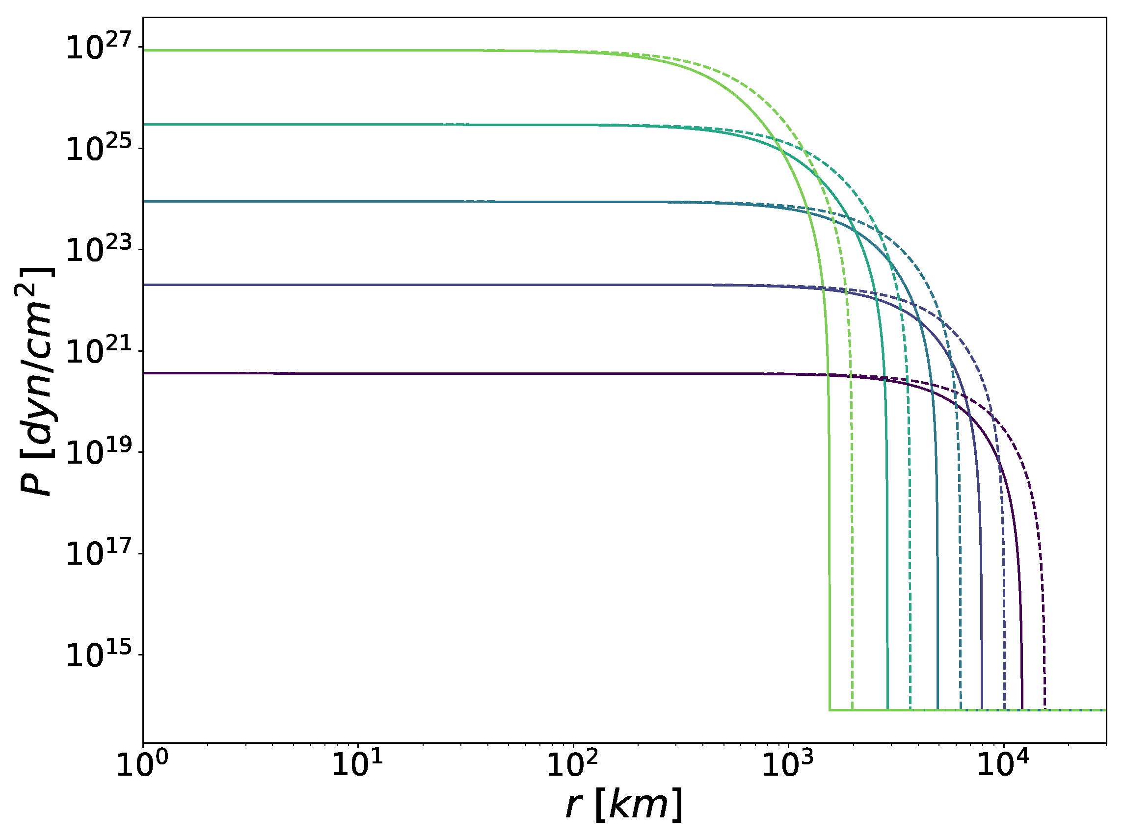
4.1. Pressure Profiles

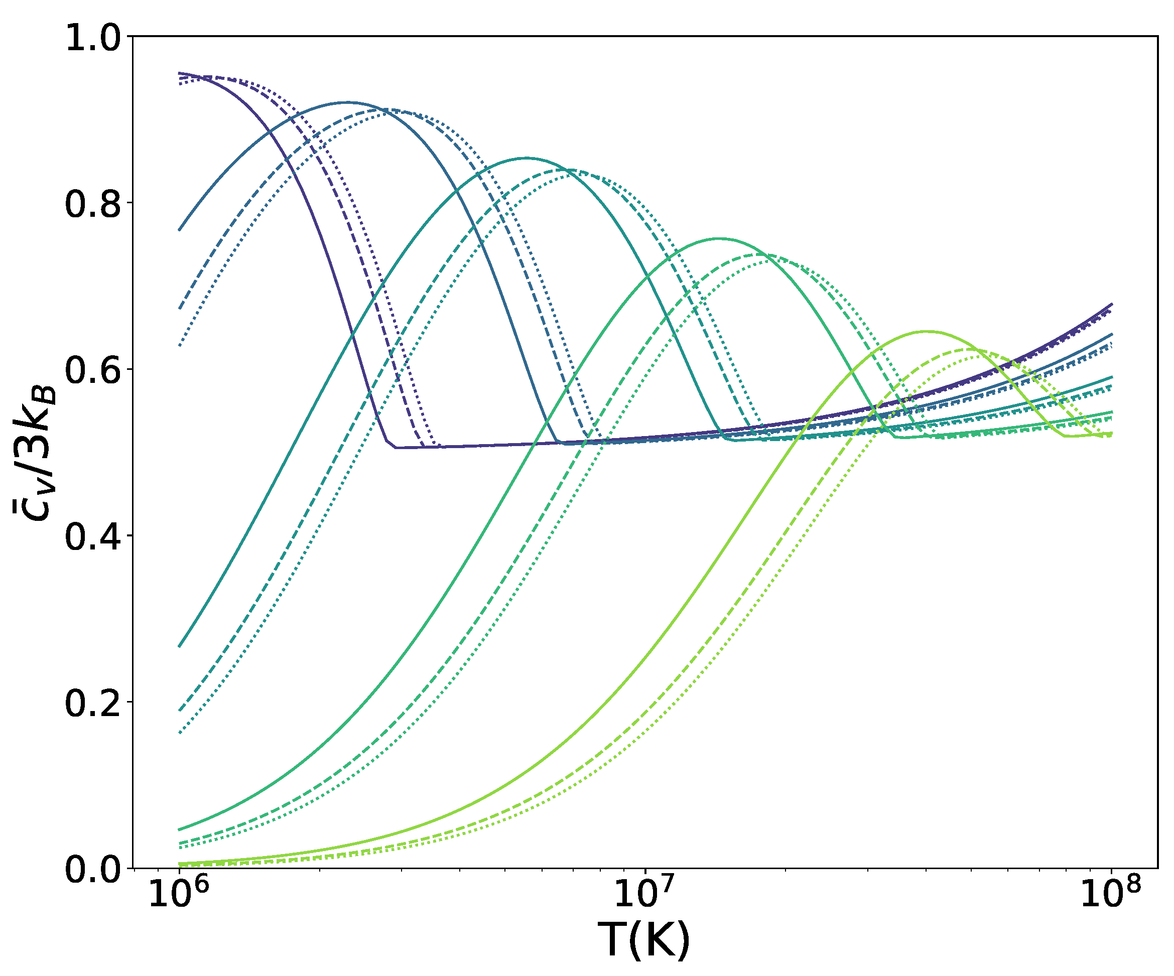
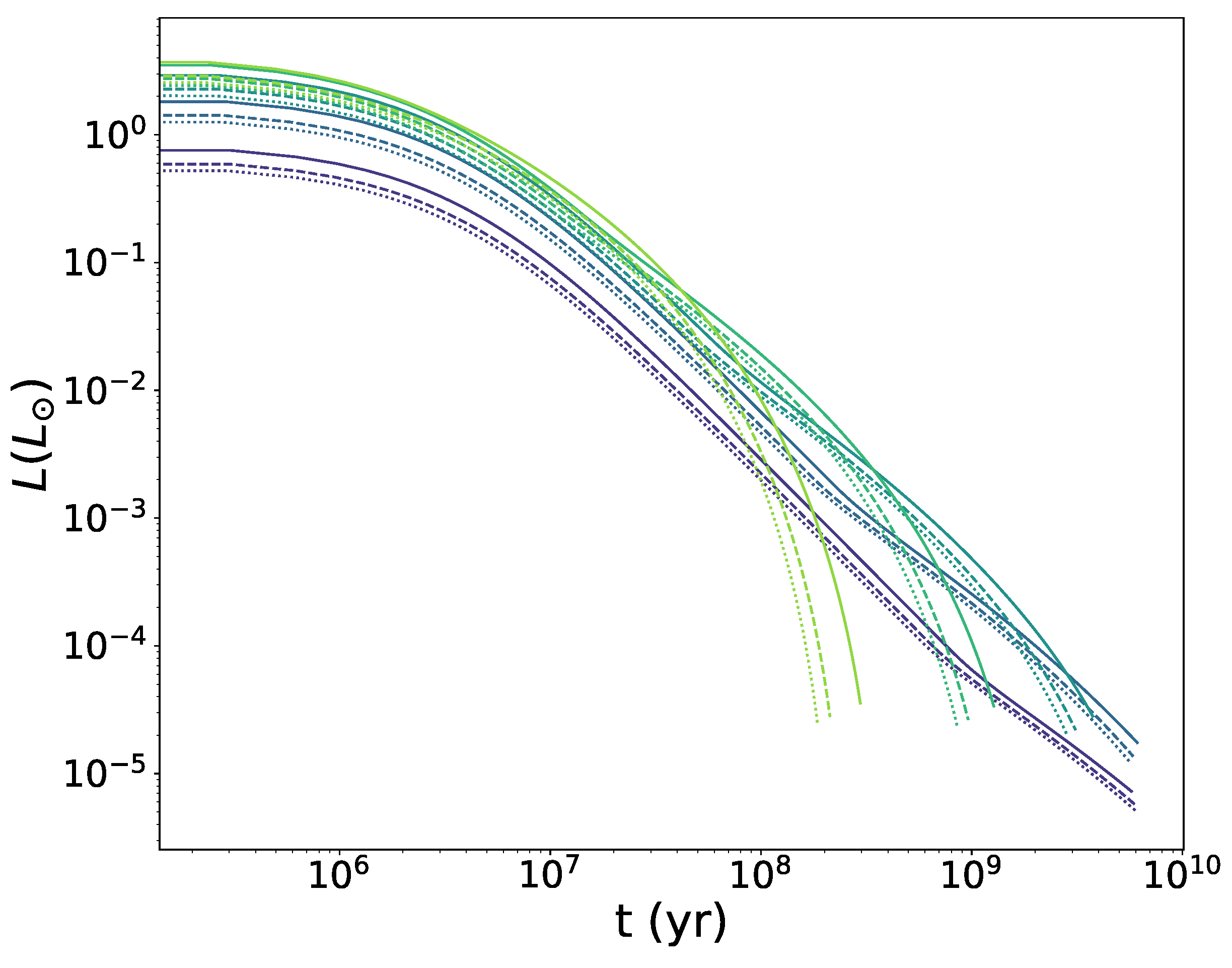
Figure 1 displays the pressure profiles $\tilde{P}\left(r\right)$ for WDs in two different chameleon models with distinct coupling strengths, namely, $\beta =0.1$ and $\beta =0.01$, while keeping the remaining parameters fixed at $n=1$ and $\Lambda ={10}^{-18}{M}_P$. For a star in GR or Newtonian gravity, the pressure $\tilde{P}$ decreases along the radius. More precisely, it drops when $r\sim {10}^3–{10}^4$ km, which is the range of the WDs’ radii. We observe that, the lower the coupling strength $\beta$, the longer it takes for the pressure to decrease. From a mathematical point of view, this is easily understood from Equation (17). For our choice of chameleon functions, the term $A_{,\varphi }/A$ is simply $\beta /M_P$. Hence, the rate at which the pressure diminishes is directly proportional to the product of $\beta$ and $\sigma$.

From a physical perspective, it is obvious that the pressure decrease will be less affected by the scalar field if the coupling between the latter and the matter is weaker, with positive coupling defined here. Regarding the scalar field gradient $\sigma$, we know it will also be positive. The scalar field has a minimum inside the star and another one outside of it, the latter being higher than the former since the outside density is lower than the inside one (recall Equation (21)). In the absence of other extrema between the minima, the scalar field exhibits a strictly increasing profile. Consequently, $\beta \sigma$ will always be positive (see Section 4.3 for computational evidence). Then, since the hydrostatic Equation (17) has a global negative sign, the scalar contribution to it will always boost the pressure decrease.

As we can already imagine, this pressure drop will cause the chameleon-screened WDs to have different masses and radii than the ones in GR or Newtonian gravity. Since the pressure—and therefore the density—falls earlier, we achieve the condition $\tilde{\rho }\left(R\right)={\tilde{\rho }}_{\infty }$ sooner; thus, we obtain a smaller stellar radius R in chameleon screening than in GR. This reduction is also translated to the stellar mass since it is defined as the mass contained in R. Accordingly, we obtain less massive stars in our chameleon model (see Section 4.4).

4.2. Cooling Time

The chameleon field will influence the thermal behaviour of WDs. To assess its impact quantitatively, we compute the stellar mean specific heat

$${\overline{c}}_V={\displaystyle \frac{1}{M}}{\int }_0^M\left(c_V^{\mathrm{ion}}+c_V^{\mathrm{el}}\right)dm,$$

(26)

where M is the mass of the WD, and $c_V^{\mathrm{ions}}$ denotes the specific heat of ions, as $c_V^{\mathrm{el}}$ does for the electrons [48]. The former depends on the ratio of Coulomb to thermal energy $\Gamma$, whose critical value is around ${\Gamma }_c=125$ [60]. If $\Gamma <{\Gamma }_c$, the ion specific heat is constant, namely, $c_V^{\mathrm{ion}}=(3/2)k_B=3/2$, and, if $\Gamma >{\Gamma }_c$, it depends on the temperature as

$$c_V^{\mathrm{ion}}=9{\left({\displaystyle \frac{T}{{\Theta }_D}}\right)}^3{\int }_0^{{\Theta }_D/T}{\displaystyle \frac{x^4{e}^x}{{(e^x-1)}^2}}dx,$$

(27)

where

$${\Theta }_D=3.48\times {10}^3{Y}_e\sqrt{\tilde{\rho }}$$

(28)

stands for the Debye temperature in K, with the stellar density expressed in $\mathrm{g}{\mathrm{cm}}^{-3}$. The electrons’ specific heat is a function temperature too [61], as follows:

$$c_V^{\mathrm{el}}={\displaystyle \frac{{\pi }^2}{2}}Z{\displaystyle \frac{T}{{\widetilde{ϵ}}_F}},$$

(29)

where ${\widetilde{ϵ}}_F={\tilde{p}}_F^2+m_e^2$ is the Fermi energy and $p_F^3=3{\pi }^2{Y}_e\tilde{\rho }/m_p$ is the Fermi momentum (recall Section 2.2), with $m_p$ being the proton mass.

The dependence of the mean specific heat on temperature for carbon WDs (recall Section 2.2) is displayed in Figure 2. We observe that the ${\overline{c}}_V-T$ curves in our ST theory are shifted to higher temperatures as compared to those in Newtonian gravity. This means that, for any given temperature T below the temperature of the ${\overline{c}}_V$ maximum, the specific heat is lower for chameleon-screened WDs. This also happens when the specific heat is dominated by the constant contribution of $c_V^{\mathrm{ion}}=3/2$ (notice the drop in all curves in Figure 2). However, between the ${\overline{c}}_V$ maximum and this drop, the specific heat for WDs in our chameleon model is higher than for their purely Newtonian counterparts. Nevertheless, the overall values of the specific heat are smaller in our ST theory, as can be appreciated by looking at the maximum of each curve: the higher the coupling strength $\beta$, the lower the ${\overline{c}}_V$ maximum. This leads to a faster WD cool-down.

To see this explicitly, we assume that the decrease over time t of the thermal energy of electrons and ions is the main source of WD luminosity L. Then, it can be expressed as follows:

$$L=-{\displaystyle \frac{M}{A{m}_p}}{\overline{c}}_V{\displaystyle \frac{dT}{dt}},$$

(30)

where T is the temperature of the star and M its mass. To integrate this ODE, we need a luminosity fit like the following (see [62] and the references therein for further examples):

$${\displaystyle \frac{L}{M}}=9.743\times {10}^{-21}{T}^{2.56}{\displaystyle \frac{L_{\odot }}{M_{\odot }}},$$

(31)

with the temperature T in K. The temporal decline of WD luminosity is displayed in Figure 3, where we have assumed an initial temperature $T_{\mathrm{ini}}={10}^{8}K$ and allowed for cooling to a final temperature $T_{\mathrm{ini}}={10}^{6}K$. The period elapsed between these two temperatures is the WD cooling time. We observe that the presence of the chameleon field makes the WDs cool faster, an effect that becomes more evident for higher densities. This indicates that the faster cooling is not entirely due to chameleon-screened WDs having lower masses. The different cooling rates displayed by low and high densities come from the fact that the specific heat for less dense WDs is approximately constant for a significant range of temperatures, as seen in Figure 2. Conversely, the strong temperature dependence that ${\overline{c}}_V$ has in dense stars gives us the faster decay in Figure 3.

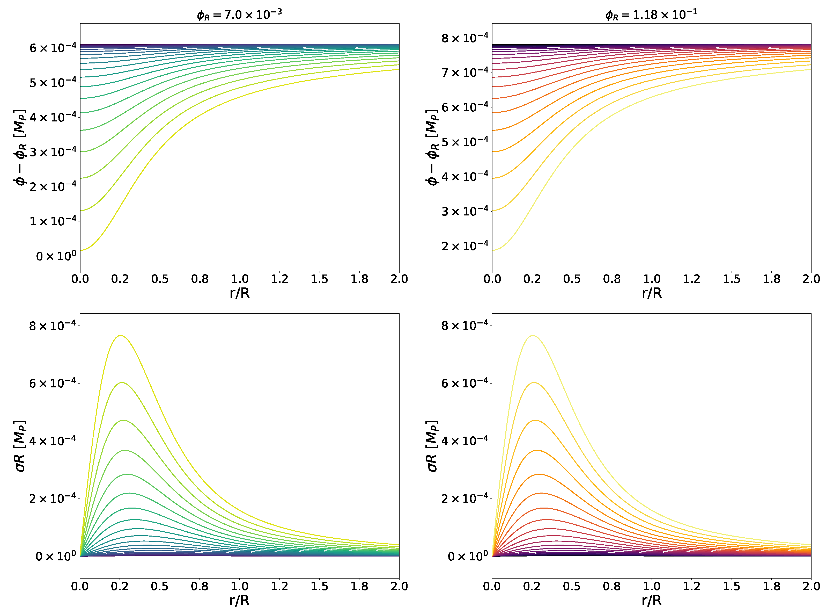
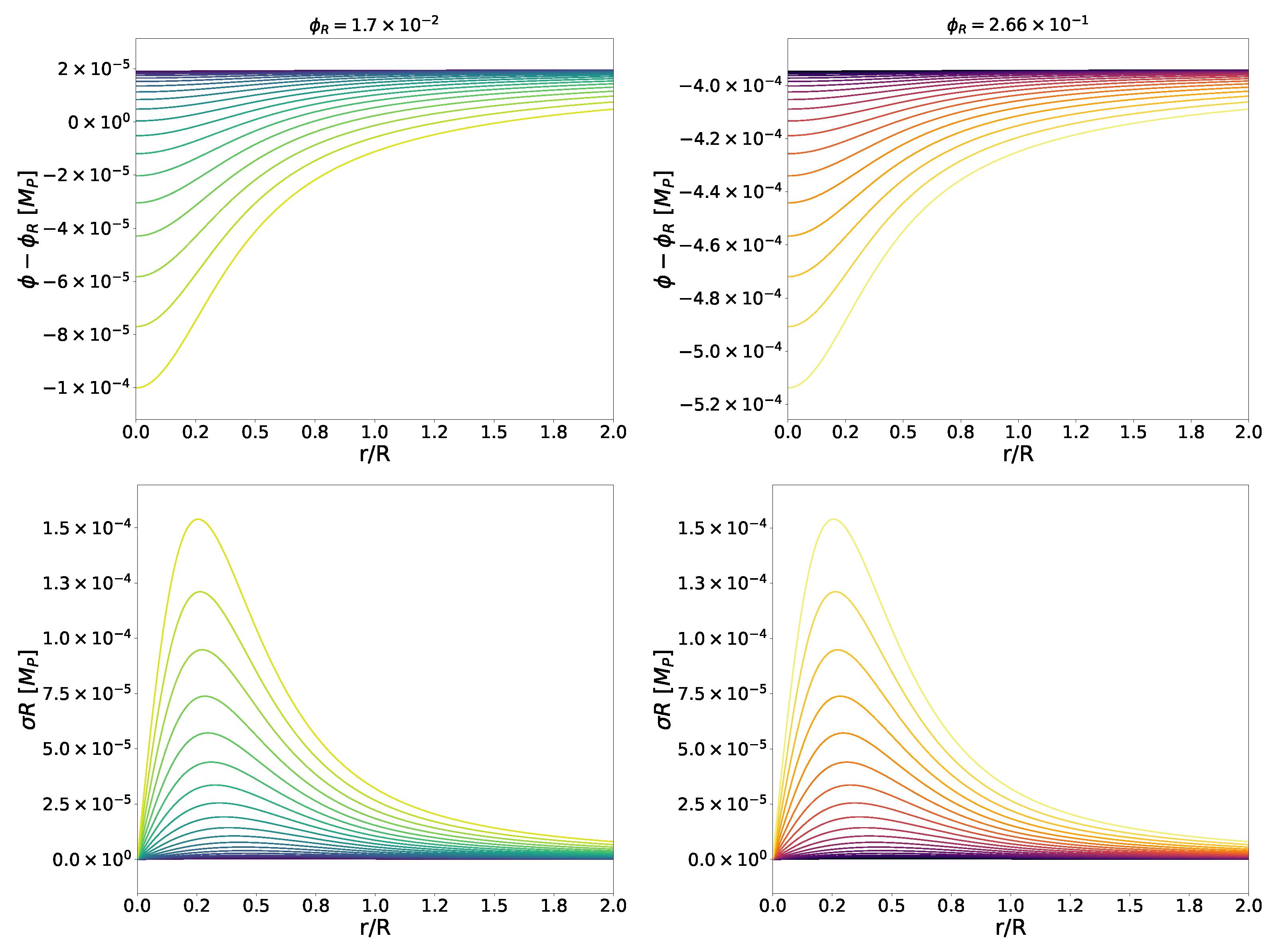
4.3. Scalar Profiles

In Figure 4, we show the radial profiles of the chameleon field $\varphi \left(r\right)$, as well as those of its gradient $\sigma \left(r\right)$, for two different parameter choices (see Equation (20)), namely, $n=1$ and $n=2$ for a fixed $\beta =0.05$ and $\Lambda ={10}^{-19}{M}_P$. In Figure 5, we plot the same radial profiles but for $\beta =0.01$. In all four cases, the field profile remains almost constant at low central densities (indicated by darker colours). As the central density increases, $\varphi$ becomes increasingly suppressed within the star, leading to the emergence of the characteristic thick-shell configuration [18]. This is the essence of the chameleon screening mechanism, as we explained in Section 3.1.

It is worth mentioning the difference in the scalar field values between the $n=1$ and $n=2$ scenarios. In both cases—see panels (a) and (b) in Figure 4 and Figure 5—the scalar field in the $n=2$ model is approximately two orders of magnitude larger than in the $n=1$ model. Yet this means that the chameleon potential $V\left(\varphi \right)$ (recall (20)) has higher values in the $n=1$ model. For instance, for the scalar field values in Figure 4, we have that $V\sim {10}^{-92}{M}_P^4$ in the $n=1$ model and that $V\sim {10}^{-113}{M}_P^4$ for $n=2$. For Figure 5, one has that $V\sim {10}^{-92}{M}_P^4$ for $n=1$ and $V\sim {10}^{-113}{M}_P^4$ for $n=2$. It seems that, for a fixed pair of $\beta$ and $\Lambda$, the scalar field potential is much more significant for $n=1$ than for $n=2$. This could lead us to think that the chameleon screening will affect the WD much more in the $n=1$ case. Still, one must not forget the gradient contribution, which, as discussed in Section 4.1, plays a crucial role in the stellar structure.

The radially normalised scalar field gradient—normalised in the sense that we have multiplied each scalar field gradient profile $\sigma \left(r\right)$ by the corresponding stellar radius R—displays similar values between the $n=1$ and the $n=2$ cases for the two considered coupling strengths (cf. the bottom panels of Figure 4 and Figure 5). We also encounter the same values in both realisations if we change the chameleon energy scale $\Lambda$. This coincidence is qualitatively explained by the approximate solution (24) presented in Section 3.1. In particular, from the top panels of Figure 4 and Figure 5, we realise that the scalar field changes throughout the whole stellar profile, being therefore in the thick-shell regime where the referred solution applies. This contrasts with solutions for more compact objects, such as neutron stars [42], which exhibit a thin-shell behaviour. 1 Deriving Equation (24) with respect to r,

$$\sigma \left(r\right)={\displaystyle \frac{\beta {\rho }_{c}r}{3M_P}},$$

(32)

and taking into account that $\sigma R$ reaches its maximum somewhere between $R/4$ and $R/2$, we have

$$\sigma \left(xR\right)={\displaystyle \frac{\beta {\rho }_{c}xR}{3M_P}}={\displaystyle \frac{\beta xM}{M_{P}4\pi R^2}}={\displaystyle \frac{2\beta x{M}_P{\Phi }_c}{R}},$$

(33)

with x being the corresponding fraction of R. Note that, in deriving this expression, we have replaced the average density with the stellar mass and radius, ${\rho }_c\equiv 3M/\left(4\pi R^3\right)$, and introduced the Newtonian potential at the surface of the star, ${\Phi }_c\equiv M/\left(8\pi M_P^{2}R\right)$. Hence, in this approximation, the maximum of $\sigma R$ depends only on the coupling strength $\beta$ and the Newtonian potential ${\Phi }_c$, that is,

$$\sigma \left(xR\right)R=2x{M}_P\beta {\Phi }_c.$$

(34)

As this result, which as explained in Section 3.1, is essentially based on neglecting the contribution of the potential as compared to the chameleon coupling function, we expected no dependence on the potential parameters n and $\Lambda$. What we did not expect was that the numerical results would also be independent of such parameters. However, it must be said that Equation (34) gives values an order of magnitude below the ones we obtained computationally. Still, the ratio between both values of the $\sigma R$ maxima is consistent through all the realisations of the chameleon model that we have studied. We find this agreement between our results and the analytical solution noteworthy.

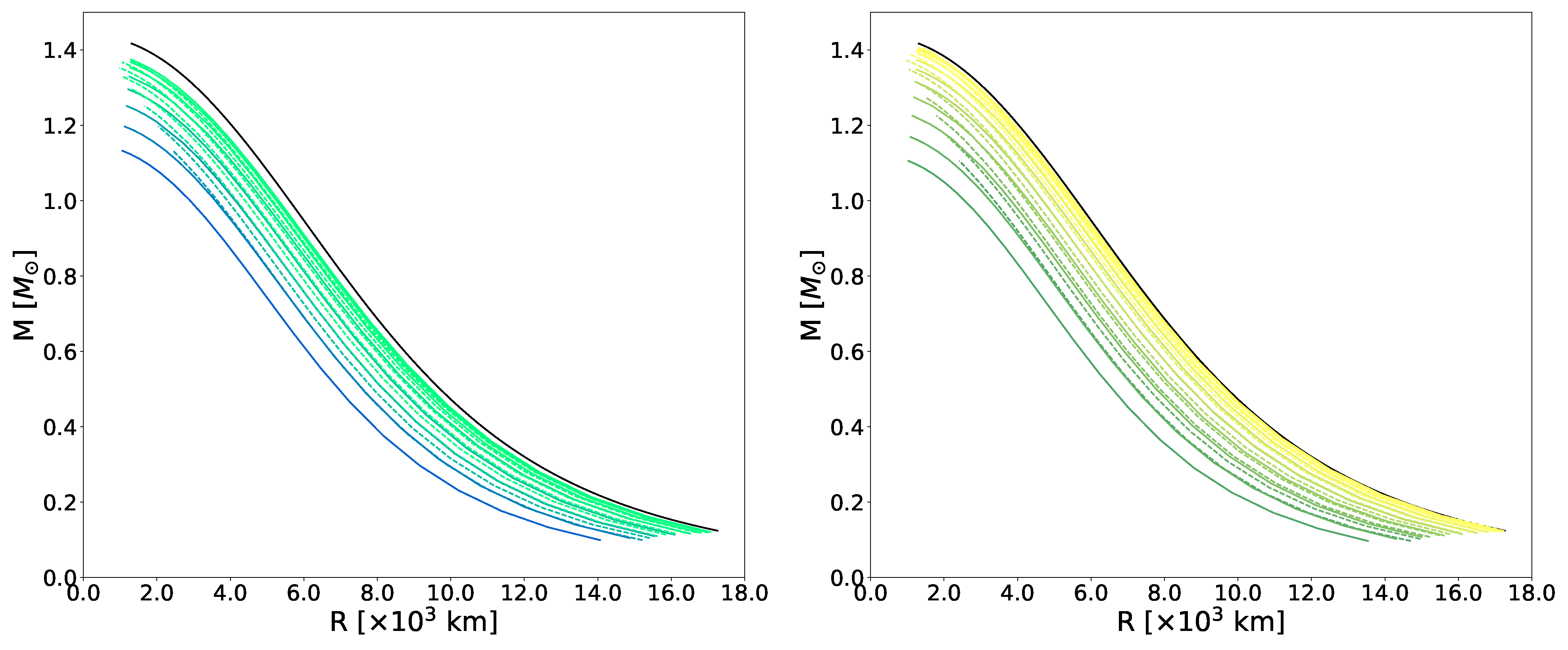
4.4. Mass–Radius Relation

Figure 6 contains numerically computed MR curves for chameleon realisations defined by the parameter values discussed at the beginning of this section with $n=1$. As anticipated from the pressure and mass profiles in Figure 1, all MR curves of chameleon-screened WDs are below (or practically on top of) the MR curve predicted by Newtonian gravity. Thus, the observed super-Chandrasekhar mass WDs [52] cannot be explained by chameleon screening. As expected, the smaller the coupling parameter $\beta$, the closer the MR curves for our ST theory are between them and the closer they are to the Newtonian one.

The MR curves for each explored value of $\beta$ tend to converge as $\Lambda$ decreases, suggesting they approach an asymptotic curve that never intersects the Newtonian one. This leads us to think that, if we were to consider much lower values of $\Lambda$, the MR curve for chameleon-screened WDs would never meet that for Newtonian WDs. Unfortunately, we need to significantly increase the numerical precision to explore such small energy scales.

Since the degeneracy between curves is evident—in the sense that we could obtain the same masses and radii with various combinations of n, $\beta$, and $\Lambda$—it is useful to obtain a parametric function for them. A relation like $R=R(M,n,\beta ,\Lambda )$ can bring order into chaos, allowing us to compare not only different chameleon realisations between themselves but also between other models, such as other ST theories with screening mechanisms. Since all the solid curves in Figure 6 appear to have the same shape, we assume this formula for the mass–radius relation [63]:

$$R=R_{*}{\left({\displaystyle \frac{M}{M_{\odot }}}\right)}^{-{\displaystyle \frac{1}{3}}}\sqrt{1-{\left({\displaystyle \frac{M}{M_{*}}}\right)}^{{\displaystyle \frac{4}{3}}}},$$

(35)

which perfectly fits the MR curve for WDs in Newtonian gravity. In that case, we have that $R_{*}=8.83\times {10}^3$ km, and the $M_{*}$ parameter naturally coincides with the Chandrasekhar mass, i.e., $M_{*}=M_{Ch}=1.45$ $M_{\odot }$.

To parametrise the MR curve of the chameleon-screened WDs, we turn the constants $R_{*}$ and $M_{*}$ into functions of the parameters of our chameleon model. Having explored the dependence of maximum radii and maximum masses with $\beta$ and $\Lambda$, we found that parabolic functions are a good ansatz, namely,

$$\begin{array}{cc}\hfill R_{*}& =R_0+A_1\beta +A_2{\beta }^2+B_1{\displaystyle \frac{\Lambda }{{\Lambda }_0}}+B_2{\left({\displaystyle \frac{\Lambda }{{\Lambda }_0}}\right)}^2,\end{array}$$

(36)

$$\begin{array}{cc}\hfill M_{*}& =M_0+C_1\beta +C_2{\beta }^2+D_1{\displaystyle \frac{\Lambda }{{\Lambda }_0}}+D_2{\left({\displaystyle \frac{\Lambda }{{\Lambda }_0}}\right)}^2,\end{array}$$

(37)

with ${\Lambda }_0={10}^{-19}{M}_P$ being a normalisation factor and $R_0$, $M_0$, $A_1$, $A_2$, $B_1$, $B_2$, $C_1$, $C_2$, $D_1$, $D_2$ constants. The best-fit values for these parameters are summarised in

Table 1. Best-fit values for the parabolic parametrisation of MR curves for chameleon-screened WDs with $n=1$, defined by Equations (35)–(37) with a coefficient of determination $R^2=0.992$. Note that $\beta \ll 1$ results in the larger values for the $A_i$ and $C_i$ coefficients.

Parameter	Value (km)	Parameter	Value (${\mathit{M}}_{\odot }$)
$R_0$	$9.638\times {10}^3$	$M_0$	$1.532$
$A_1$	$-2.005\times {10}^4$	$C_1$	$-1.919$
$A_2$	$1.066\times {10}^5$	$C_2$	$7.528$
$B_1$	$-1.434\times {10}^2$	$D_1$	$-1.179\times {10}^{-2}$
$B_2$	$-5.941$	$D_2$	$-1.080\times {10}^{-3}$

, with a coefficient of determination $R^2=0.992$. The corresponding curves are shown in Figure 6, with the same colouring as their numerical counterparts. As is apparent in these plots, the agreement between the numerics and fitting formulae is sufficient for all practical purposes.

5. Conclusions

In this work, we have studied the behaviour of the chameleon field around WDs and its possible effects on their structure and characteristics. They are promising candidates for testing alternative theories of gravity since there are extensive observational data available, and we have a sensible grasp of the EoS describing the matter within them. We have shown that the Newtonian approximation accurately describes WDs in this particular kind of ST theory, as happens in GR. Assuming a Chandrasekhar EoS, we implemented a tailored shooting method to solve the equilibrium equations.

We saw that the presence of the chameleon field affects the WD’s pressure gradient, causing the pressure to drop prematurely as compared to when there is no scalar field. This leads to smaller stellar masses and radii which, in turn, shifts the MR curves below the MR relation predicted by Newtonian gravity. However, those stars above the theoretical curve—which are the majority—cannot come from any chameleon realisation, being therefore necessary to invoke other mechanisms such as strong magnetic fields [64,65] or inverse chameleon settings [66].

The existence of a chameleon field alters the specific heat of WDs too, lowering their values and reducing their cooling times. We have shown this effect to be more pronounced for denser stars and stronger $\beta$ couplings, confirming the role of the scalar field in the cooling process, which turns out to be not just a direct consequence of the smaller stellar masses of the chameleon-screened WDs.

We examined the radial profiles of the scalar field and its gradient, considering a wide range of numerically feasible values for the model parameters—the energy scale $\Lambda$ and the coupling strength $\beta$—and showing, for the first time in the literature, $n=2$ realisations of the chameleon. This allowed us to identify a similarity relation of the chameleon theory for the radially normalised scalar field gradient, that is $\sigma R$. In the thick-shell regime of the chameleon screening, the maximum $\sigma R$ is determined solely by $\beta$, and we encountered the same behaviour in our numerical results, independent of the $\Lambda$ and n values considered.

After exploring the ranges of the chameleon energy scales and coupling strengths, we inferred parametric expressions for the MR relations that depend on the mentioned parameters. This result allowed us to check for degeneracies between other classes of screening mechanisms once the analogous formulae were derived without having to numerically solve the ODE systems again, a computationally time-consuming task.

A continuation of this work could be to explore the stability of chameleon-screened WDs through radial and non-radial pulsation modes, or even to study the stable regime of WD oscillations [67]. Incorporating EoSs with leading-order Coulomb interactions, finite-temperature corrections, and stellar envelope contributions could be a future research direction. Naturally, an interesting prospect would be to apply the presented framework and the developed computational tools to other ST theories.

Still, a consistent ST treatment of WD would demand MG simulations—a currently unavailable but crucial ingredient [46]. A sensible comparison with observational data is only attainable once the systematic effects are adequately accounted for. For example, independent measurements of the mass, radius, and effective temperature of WDs from eclipsing binary systems are essential for mitigating degeneracies and reducing observational uncertainties. For instance, uncertainties in mass and radius measurements of WDs [52] are sufficiently large to encompass the MR curves presented in Figure 6, rendering distinctions between model realisations observationally inconclusive. Furthermore, comparing our WD cooling curves with data from stellar clusters would require translating our luminosity outputs into absolute magnitude–colour diagrams. This, in turn, demands adopting detailed atmospheric models [53], introducing further model-dependent uncertainties. In the literature, cooling times are typically inferred by assuming specific white dwarf structures—such as models with hydrogen-dominated (DA) or helium-dominated (DB) atmospheres with carbon–oxygen or oxygen–neon cores—and by relying on evolutionary sequences developed by particular research groups. The choice of atmospheric model and input physics can significantly affect the derived ages. Reported uncertainties are often large and vary across clusters such as Coma Ber, Hyades, M67, the Pleiades, and Praesepe [68,69,70,71,72]. Moreover, the variation between cooling tracks of different WD types in the aforementioned magnitude–colour diagrams can be more significant than the chameleon-induced deviations presented here. Incidentally, direct comparison of our luminosity evolution with curves belonging to observed WDs encounters the same issue [73]: model-dependent uncertainties are too large to allow for a consistent comparison between our theoretical results and observations. For these reasons—and considering that our results are based on scalar field parameters chosen for numerical feasibility (see Section 4.3)—we have refrained from comparing our results with observational data.

References

1. Will, C.M. Theory and Experiment in Gravitational Physics; Cambridge University Press: Cambridge, UK, 2018. [Google Scholar]
2. Clifton, T.; Ferreira, P.G.; Padilla, A.; Skordis, C. Modified Gravity and Cosmology. Phys. Rep. 2012, 513, 1–189. [Google Scholar] [CrossRef]
3. Burrage, C.; Sakstein, J. Tests of chameleon gravity. Living Rev. Relativ. 2018, 21, 1. [Google Scholar] [CrossRef] [PubMed]
4. Brax, P.; Casas, S.; Desmond, H.; Elder, B. Testing Screened Modified Gravity. Universe 2021, 8, 11. [Google Scholar] [CrossRef]
5. Fischer, H.; Käding, C.; Pitschmann, M. Screened Scalar Fields in the Laboratory and the Solar System. Universe 2024, 10, 297. [Google Scholar] [CrossRef]
6. Amendola, L.; Rubio, J.; Wetterich, C. Primordial black holes from fifth forces. Phys. Rev. D 2018, 97, 81302. [Google Scholar] [CrossRef]
7. Savastano, S.; Amendola, L.; Rubio, J.; Wetterich, C. Primordial dark matter halos from fifth forces. Phys. Rev. D 2019, 100, 83518. [Google Scholar] [CrossRef]
8. Goh, L.W.K.; Bachs-Esteban, J.; Gómez-Valent, A.; Pettorino, V.; Rubio, J. Observational constraints on early coupled quintessence. Phys. Rev. D 2024, 109, 23530. [Google Scholar] [CrossRef]
9. Wetterich, C. The Cosmon model for an asymptotically vanishing time dependent cosmological ‘constant’. Astron. Astrophys. 1995, 301, 321–328. [Google Scholar] [CrossRef]
10. Wetterich, C. Growing neutrinos and cosmological selection. Phys. Lett. B 2007, 655, 201–208. [Google Scholar] [CrossRef]
11. Amendola, L.; Baldi, M.; Wetterich, C. Quintessence cosmologies with a growing matter component. Phys. Rev. D 2008, 78, 23015. [Google Scholar] [CrossRef]
12. Casas, S.; Pettorino, V.; Wetterich, C. Dynamics of neutrino lumps in growing neutrino quintessence. Phys. Rev. D 2016, 94, 103518. [Google Scholar] [CrossRef]
13. Garcia-Bellido, J.; Rubio, J.; Shaposhnikov, M.; Zenhausern, D. Higgs-Dilaton Cosmology: From the Early to the Late Universe. Phys. Rev. D 2011, 84, 123504. [Google Scholar] [CrossRef]
14. Ferreira, P.G.; Hill, C.T.; Ross, G.G. No fifth force in a scale invariant universe. Phys. Rev. D 2017, 95, 64038. [Google Scholar] [CrossRef]
15. Casas, S.; Karananas, G.K.; Pauly, M.; Rubio, J. Scale-invariant alternatives to general relativity. III. The inflation-dark energy connection. Phys. Rev. D 2019, 99, 63512. [Google Scholar] [CrossRef]
16. Copeland, E.J.; Millington, P.; Muñoz, S.S. Fifth forces and broken scale symmetries in the Jordan frame. JCAP 2022, 2, 16. [Google Scholar] [CrossRef]
17. Khoury, J.; Weltman, A. Chameleon Fields: Awaiting Surprises for Tests of Gravity in Space. Phys. Rev. Lett. 2004, 93, 171104. [Google Scholar] [CrossRef] [PubMed]
18. Khoury, J.; Weltman, A. Chameleon cosmology. Phys. Rev. D 2004, 69, 44026. [Google Scholar] [CrossRef]
19. Brax, P.; van de Bruck, C.; Davis, A.-C.; Khoury, J.; Weltman, A. Detecting dark energy in orbit: The cosmological chameleon. Phys. Rev. D 2004, 70, 123518. [Google Scholar] [CrossRef]
20. Chou, A.S.; Wester, W.; Baumbaugh, A.; Gustafson, H.R.; Irizarry-Valle, Y.; Mazur, P.O.; Steffen, J.H.; Tomlin, R.; Upadhye, A.; Weltman, A.; et al. Search for Chameleon Particles Using a Photon-Regeneration Technique. Phys. Rev. Lett. 2009, 102, 30402. [Google Scholar] [CrossRef] [PubMed]
21. Steffen, J.H.; Upadhye, A.; Baumbaugh, A.; Chou, A.S.; Mazur, P.O.; Tomlin, R.; Weltman, A.; Wester, W. Laboratory Constraints on Chameleon Dark Energy and Power-Law Fields. Phys. Rev. Lett. 2010, 105, 261803. [Google Scholar] [CrossRef] [PubMed]
22. Hinterbichler, K.; Khoury, J. Screening Long-Range Forces through Local Symmetry Restoration. Phys. Rev. Lett. 2010, 104, 231301. [Google Scholar] [CrossRef] [PubMed]
23. Hinterbichler, K.; Khoury, J.; Levy, A.; Matas, A. Symmetron Cosmology. Phys. Rev. D 2011, 84, 103521. [Google Scholar] [CrossRef]
24. Högås, M.; Mörtsell, E. Impact of symmetron screening on the Hubble tension: New constraints using cosmic distance ladder data. Phys. Rev. D 2023, 108, 024007. [Google Scholar] [CrossRef]
25. Brax, P.; van de Bruck, C.; Davis, A.C.; Shaw, D. The Dilaton and Modified Gravity. Phys. Rev. D 2010, 82, 63519. [Google Scholar] [CrossRef]
26. Fischer, H.; Käding, C.; Sedmik, R.I.P.; Abele, H.; Brax, P.; Pitschmann, M. Search for environment-dependent dilatons. Phys. Dark Universe 2024, 43, 101419. [Google Scholar] [CrossRef]
27. Brax, P.; Fischer, H.; Käding, C.; Pitschmann, M. The environment dependent dilaton in the laboratory and the solar system. Eur. Phys. J. C 2022, 82, 934. [Google Scholar] [CrossRef] [PubMed]
28. Vainshtein, A.I. To the problem of nonvanishing gravitation mass. Phys. Lett. B 1972, 39, 393–394. [Google Scholar] [CrossRef]
29. Burrage, C.; Coltman, B.; Padilla, A.; Saadeh, D.; Wilson, T. Massive Galileons and Vainshtein screening. J. Cosmol. Astropart. Phys. 2021, 2021, 50. [Google Scholar] [CrossRef]
30. Babichev, E.; Deffayet, C.; Ziour, R. k-Mouflage gravity. Int. J. Mod. Phys. D 2009, 18, 2147–2154. [Google Scholar] [CrossRef]
31. Brax, P.; Valageas, P. The effective field theory of K-mouflage. J. Cosmol. Astropart. Phys. 2016, 2016, 20. [Google Scholar] [CrossRef]
32. Brax, P.; Burrage, C.; Davis, A.-C. Screening fifth forces in k-essence and DBI models. J. Cosmol. Astropart. Phys. 2013, 1, 20. [Google Scholar] [CrossRef]
33. ter Haar, L.; Bezares, M.; Crisostomi, M.; Barausse, E.; Palenzuela, C. Dynamics of Screening in Modified Gravity. Phys. Rev. Lett. 2021, 126, 91102. [Google Scholar] [CrossRef] [PubMed]
34. Luongo, O.; Mengoni, T. Generalized K-essence inflation in Jordan and Einstein frames. Class. Quantum Gravity 2024, 41, 105006. [Google Scholar] [CrossRef]
35. D’Agostino, R.; Luongo, O.; Muccino, M. Healing the cosmological constant problem during inflation through a unified quasi-quintessence matter field. Class. Quantum Gravity 2022, 39, 195014. [Google Scholar] [CrossRef]
36. Babichev, E.; Langlois, D. Relativistic stars in f(R) and scalar-tensor theories. Phys. Rev. D 2010, 81, 124051. [Google Scholar] [CrossRef]
37. Chang, P.; Hui, L. Stellar Structure and Tests of Modified Gravity. Astrophys. J. 2011, 732, 25. [Google Scholar] [CrossRef]
38. Sakstein, J. Stellar oscillations in modified gravity. Phys. Rev. D 2013, 88, 124013. [Google Scholar] [CrossRef]
39. Brito, R.; Terrana, A.; Johnson, M.; Cardoso, V. Nonlinear dynamical stability of infrared modifications of gravity. Phys. Rev. D 2014, 90, 124035. [Google Scholar] [CrossRef]
40. Babichev, E.; Koyama, K.; Langlois, D.; Saito, R.; Sakstein, J. Relativistic Stars in Beyond Horndeski Theories. Class. Quant. Grav. 2016, 33, 235014. [Google Scholar] [CrossRef]
41. Brax, P.; Davis, A.C.; Jha, R. Neutron Stars in Screened Modified Gravity: Chameleon vs Dilaton. Phys. Rev. D 2017, 95, 83514. [Google Scholar] [CrossRef]
42. de Aguiar, B.F.; Mendes, R.F. Highly compact neutron stars and screening mechanisms: Equilibrium and stability. Phys. Rev. D 2020, 102, 24064. [Google Scholar] [CrossRef]
43. de Aguiar, B.F.; Mendes, R.F.P.; Falciano, F.T. Neutron Stars in the Symmetron Model. Universe 2021, 8, 6. [Google Scholar] [CrossRef]
44. Panotopoulos, G.; Rubio, J.; Lopes, I. On the impact of nonlocal gravity on compact stars. Int. J. Mod. Phys. D 2023, 32, 2250139. [Google Scholar] [CrossRef]
45. Dima, A.; Bezares, M.; Barausse, E. Dynamical chameleon neutron stars: Stability, radial oscillations, and scalar radiation in spherical symmetry. Phys. Rev. D 2021, 104, 84017. [Google Scholar] [CrossRef]
46. Saltas, I.D.; Sawicki, I.; Lopes, I. White dwarfs and revelations. J. Cosmol. Astropart. Phys. 2018, 2018, 28. [Google Scholar] [CrossRef]
47. Alam, K.; Islam, T. White dwarf mass-radius relation in theories beyond general relativity. JCAP 2023, 8, 81. [Google Scholar] [CrossRef]
48. Kalita, S.; Sarmah, L.; Wojnar, A. Metric-affine effects in crystallization processes of white dwarfs. Phys. Rev. D 2023, 107, 44072. [Google Scholar] [CrossRef]
49. Vidal, S.; Wojnar, A.; Järv, L.; Doneva, D. Crystallized white dwarf stars in scalar-tensor gravity. Phys. Rev. D 2025, 111, 84075. [Google Scholar] [CrossRef]
50. Bachs-Esteban, J.; Lopes, I.; Rubio, J. Screening Mechanisms on White Dwarfs: Symmetron and Dilaton. Universe 2025, 11, 158. [Google Scholar] [CrossRef]
51. Camenzind, M. Compact Objects in Astrophysics. White Dwarfs, Neutron Stars and Black Holes; Springer: Berlin/Heidelberg, Germany, 2007. [Google Scholar]
52. Jiménez-Esteban, F.M.; Torres, S.; Rebassa-Mansergas, A.; Skorobogatov, G.; Solano, E.; Cantero, C.; Rodrigo, C. A white dwarf catalogue from Gaia-DR2 and the Virtual Observatory. Mon. Not. R. Astron. Soc. 2018, 480, 4505–4518. [Google Scholar] [CrossRef]
53. Tremblay, P.E.; Cukanovaite, E.; Gentile Fusillo, N.P.; Cunningham, T.; Hollands, M.A. Fundamental parameter accuracy of DA and DB white dwarfs in Gaia Data Release 2. Mon. Not. R. Astron. Soc. 2018, 482, 5222–5232. [Google Scholar] [CrossRef]
54. Kilic, M.; Bergeron, P.; Kosakowski, A.; Brown, W.R.; Agüeros, M.A.; Blouin, S. The 100 pc White Dwarf Sample in the SDSS Footprint. Astrophys. J. 2020, 898, 84. [Google Scholar] [CrossRef]
55. Bettoni, D.; Rubio, J. Quintessential Inflation: A Tale of Emergent and Broken Symmetries. Galaxies 2022, 10, 22. [Google Scholar] [CrossRef]
56. Chandrasekhar, S. The highly collapsed configurations of a stellar mass (Second paper). Mon. Not. Roy. Astron. Soc. 1935, 95, 207–225. [Google Scholar] [CrossRef]
57. Hamada, T.; Salpeter, E.E. Models for Zero-Temperature Stars. Astrophys. J. 1961, 134, 683. [Google Scholar] [CrossRef]
58. Fontaine, G.; Brassard, P.; Bergeron, P. The Potential of White Dwarf Cosmochronology. Publ. Astron. Soc. Pac. 2001, 113, 409. [Google Scholar] [CrossRef]
59. Misner, C.W.; Thorne, K.S.; Wheeler, J.A. Gravitation; W. H. Freeman: San Francisco, CA, USA, 1973. [Google Scholar]
60. Brush, S.G.; Sahlin, H.L.; Teller, E. Monte Carlo Study of a One-Component Plasma. I. J. Chem. Phys. 1966, 45, 2102–2118. [Google Scholar] [CrossRef]
61. Koester, D. Outer Envelopes and Cooling of White Dwarfs. Astron. Astrophys. 1972, 16, 459. [Google Scholar]
62. Koester, D.; Chanmugam, G. Physics of white dwarf stars. Rep. Prog. Phys. 1990, 53, 837. [Google Scholar] [CrossRef]
63. Greiner, W.; Neise, L.; Stöcker, H. Thermodynamics and Statistical Mechanics; Springer: Berlin/Heidelberg, Germany, 1995. [Google Scholar]
64. Das, U.; Mukhopadhyay, B. Maximum mass of stable magnetized highly super-Chandrasekhar white dwarfs: Stable solutions with varying magnetic fields. JCAP 2014, 6, 50. [Google Scholar] [CrossRef]
65. Roy, S.K.; Mukhopadhyay, S.; Lahiri, J.; Basu, D.N. Relativistic Thomas-Fermi equation of state for magnetized white dwarfs. Phys. Rev. D 2019, 100, 63008. [Google Scholar] [CrossRef]
66. Wei, H.; Yu, Z.-X. Inverse chameleon mechanism and mass limits for compact stars. JCAP 2021, 8, 11. [Google Scholar] [CrossRef]
67. Sotani, H.; Kokkotas, K.D. Stellar oscillations in scalar-tensor theory of gravity. Phys. Rev. D 2005, 71, 124038. [Google Scholar] [CrossRef]
68. Dobbie, P.D.; Casewell, S.L.; Burleigh, M.R.; Boyce, D.D. A massive white dwarf member of the Coma Berenices open cluster. Mon. Not. R. Astron. Soc. 2009, 395, 1591–1598. [Google Scholar] [CrossRef]
69. Salaris, M.; Bedin, L.R. A Gaia DR2 view of white dwarfs in the Hyades. Mon. Not. R. Astron. Soc. 2018, 480, 3170–3176. [Google Scholar] [CrossRef]
70. Richer, H.B.; Fahlman, G.G.; Rosvick, J.; Ibata, R. The White Dwarf Cooling Age of M67. Astrophys. J. 1998, 504, L91–L94. [Google Scholar] [CrossRef]
71. Heyl, J.; Caiazzo, I.; Richer, H.B. Reconstructing the Pleiades with Gaia EDR3. Astrophys. J. 2022, 926, 132. [Google Scholar] [CrossRef]
72. Dobbie, P.D.; Pinfield, D.J.; Napiwotzki, R.; Hambly, N.C.; Burleigh, M.R.; Barstow, M.A.; Jameson, R.F.; Hubeny, I. Praesepe and the seven white dwarfs. Mon. Not. R. Astron. Soc. 2004, 355, L39–L43. [Google Scholar] [CrossRef]
73. Isern, J.; Artigas, A.; García-Berro, E. White dwarf cooling sequences and cosmochronology. EPJ Web Conf. 2013, 43, 5002. [Google Scholar] [CrossRef]
74. Carvalho, G.A.; Marinho, R.M.; Malheiro, M. General relativistic effects in the structure of massive white dwarfs. Gen. Relativ. Gravit. 2018, 50, 4. [Google Scholar] [CrossRef]
Figure 1. Pressure profiles of chameleon-screened WDs. We consider the chameleon model (20) with n = 1 , Λ = 10 18 M P , and β = 0.1 (solid) and β = 0.01 (dashed). Colours from purple to green denote rising central densities, specifically for ρ ˜ 0 = 7.0 × 10 4 , 8.5 × 10 5 , 1.0 × 10 7 , 1.2 × 10 8 , 1.5 × 10 9 g cm 3 . The lower the coupling strength β , the longer it takes for the pressure to decrease.
Universe 11 00237 g001
Figure 2. Stellar mean specific heat c ¯ V with respect to temperature T for chameleon-screened WDs. We consider the chameleon model (20) with n = 1 , Λ = 10 18 M P , and β = 0.1 (dotted) and β = 0.05 (dashed). For reference, we include the results for WDs in Newtonian gravity (solid). Colours from purple to green denote rising central densities, specifically ρ ˜ 0 = 4.5 × 10 5 , 5.5 × 10 6 , 6.7 × 10 7 , 8.2 × 10 8 , 1.0 × 10 10 g cm 3 . For higher values of the coupling strength β , the c ¯ V maximum decreases and the entire curve shifts to higher temperatures.
Universe 11 00237 g002
Figure 3. Luminosity L over time t for chameleon-screened WDs. We consider the chameleon model (20) with n = 1 , Λ = 10 18 M P , and β = 0.1 (dotted) and β = 0.05 (dashed). We also display the results for Newtonian gravity WDs (solid). Colours from purple to green denote rising central densities, namely, ρ ˜ 0 = 4.5 × 10 5 , 5.5 × 10 6 , 6.7 × 10 7 , 8.2 × 10 8 , 1.0 × 10 10 g cm 3 . The higher the coupling strength β , the faster the WD cools down.
Universe 11 00237 g003
Figure 4. Top panels: Scalar field radial profiles. Notice that the labels indicate the difference between the scalar field and a reference value since the variation is small compared to the latter. Bottom panels: Scalar field gradient radial profiles. The radial coordinate has been normalised to the respective stellar radius R for each curve. We consider the chameleon model (20) with Λ = 10 19 M P , β = 0.05 , and n = 1 (left panels, green tones) and n = 2 (right panels, orange tones). Tones from dark to bright denote rising central densities from ρ ˜ 0 , min = 7 × 10 4 g cm 3 to ρ ˜ 0 , max = 10 10 g cm 3 .
Universe 11 00237 g004
Figure 5. Top panels: Scalar field radial profiles. Notice that the labels indicate the difference between the scalar field and a reference value since the variation is small compared to the latter. Bottom panels: Scalar field gradient radial profiles. The radial coordinate has been normalised to the respective stellar radius R for each curve. We consider the chameleon model (20) with Λ = 10 19 M P , β = 0.01 , and n = 1 (left panels, green tones) and n = 2 (right panels, orange tones). Tones from dark to bright denote rising central densities from ρ ˜ 0 , min = 7 × 10 4 g cm 3 to ρ ˜ 0 , max = 10 10 g cm 3 .
Universe 11 00237 g005
Figure 6. Theoretical (solid) and parametric (dashed) MR curves for chameleon-screened WDs for n = 1 and different values of β and Λ , the latter changing in 10 19   M P steps. We also include the WD MR curve in Newtonian gravity (black). Left panel: β = 0.1 , Λ = 1 8 × 10 19   M P (green to blue). Right panel: β = 0.05 , Λ = 1 10 × 10 19   M P (yellow to green).
Universe 11 00237 g006