Relationship Between Recurrent Magnetic Flux Rope and Moving Magnetic Features

Abstract

Large-scale magnetic flux ropes (MFRs) usually become visible during an eruption and are the core structures of coronal mass ejections, but the nature of MFRs is still a mystery. Here, we identify a large transequatorial MFR that spans across NOAA 13373 (in the Northern Hemisphere) and NOAA 13374 (in the Southern Hemisphere). Here, NOAA 13373 is a growing, newly emerging active region with a leading sunspot moving rapidly to the southwest, and it is surrounded by a highly dynamic moving magnetic feature (MMF), while NOAA 13374 is a decaying active region with a tiny leading negative sunspot and a large fading area. Recurrent reconnection, which occurs under the MFRs around the leading sunspot of NOAA 13373, results in local energy release, appearing as local EUV brightening, and it is related to the appearance of a transequatorial MFR. The appearance of this MFR involves several stages: EUV brightening, the slow rising and expansion of the MFR and its hosted filament, and, eventually, fading and shrinking. These observations demonstrate that a large-scale MFR can exist for a long-term period and that MMFs play a key role in building up free energy and triggering small-scale reconnections in the lower atmosphere. The energy released by these reconnection events is insufficient for triggering the eruption of an MFR but results in local disturbances.

1. Introduction

A solar active region is a region with concentrated magnetic fields that emerges from the inside convection zone and extends up into the solar atmosphere. It is the main source of major solar eruptions and, to some extent, affects coronal structure. Various visible and invisible connections between active regions make solar activity more complex and harder to predict.

The most common connection between two active regions is the coronal loop, which usually can be easily identified by radio, X-ray, or EUV imaging observations [1,2,3]. The coronal loop may result in some complex activities in the solar atmosphere, such as sympathetic flares [4,5,6], the remote brightening of flares [7], filament eruption [8], and coronal mass ejections (CMEs; [9]). Ref. [10] presents observational evidence of magnetic helicity transfer from a late-emerging active region to a neighboring active region via unbalanced magnetic torque along the coronal loop. Although few in number, there are also other types of connections in the solar atmosphere. Based on the observations of a very long filament channel running through six active regions, ref. [11] studied the temporal evolution of these active regions, including the chirality in three major active regions and their associated magnetic clouds, and suggested that a large-scale intercoupled magnetic flux system may build a magnetic connection among the six associated active regions.

A magnetic flux rope (MFR), which is the possible core structure of a coronal mass ejection (CME), is usually located along a strongly sheared, highly gradient polarity inversion line (PIL) within the active region. Ref. [12] presents a large-scale eruption originating from a large-scale hot channel/MFR, which connects an anti-Hale active region and a normal active region. Though a statistical study, ref. [13] points out that all the host regions of CMEs are enveloped in large-scale magnetic structures. Their study suggests that large-scale MFRs may play a key role in large-scale eruptions. So far, studies focusing on large-scale MFRs have been rare.

Moving magnetic features (MMFs) were first revealed by [14] in 1969. They appear as small, isolated single or dipole magnetic elements around the outer penumbra, move radially outward into the moat regions, and eventually disappear in network fields or are canceled out by the opposite magnetic polarities nearby. MMFs appear in the highly dynamic zones around sunspots. Several numerical simulations and observational studies have demonstrated that MMFs might accumulate magnetic free energy to facilitate magnetic reconnection (e.g., [15,16,17,18,19]), which naturally accompanies solar activities such as jets [20], flares [21], filament eruptions, and CMEs [21].

This work investigates the recurrence of a transequatorial MFR, which connects NOAA 13373 (Northern Hemisphere) and NOAA 13374 (Southern Hemisphere). The data and observations are described in Section 2. The analyses and observational results are presented in Section 3, and the conclusions are summarized in Section 4.

2. Data and Observations

Continuum images showing the temporal evolution of sunspots were obtained with a full-disk magnetogram (FMG [22]) instrument onboard the Advanced Space-Based Solar Observatory (ASO-S [23]). The spatial and temporal resolution of the FMG is about 1 arcsecond and 2 min, respectively.

Full-disk solar images at ultraviolet (UV) and extreme ultraviolet (EUV) wavelengths were provided by the Solar Dynamics Observatory’s (SDO [24]) Atmospheric Imaging Assembly (AIA [25]), with pixel size and temporal resolution of 0.6 arcseconds and 12 s. The AIA’s 1600 Å UV band-pass is designed to observe the upper photosphere. In this study, the AIA’s 1600 Å images show the initial brightening of solar activities. For the EUV band, six band-passes (171, 193, 211, 335, 94, and 131 Å) observed the Sun from the transition region to the corona and also focused on the flaring region, with a temperature range from 0.6 to 10.0 MK. Here, we checked all EUV channels, with a particular emphasis on the AIA’s 171 and 94 Å channels. The 171 Å band-pass is sensitive to relatively cool coronal plasma (peak temperature responses of ~0.6 MK), and the 94 Å band-pass is selected for hot coronal plasma (peak temperature response of ~6.3 MK in flaring regions). The simultaneous photospheric magnetic field is obtained with a Helioseismic and Magnetic Imager (HMI [26]). The HMI on board the SDO provides the full-disk magnetic field of the Sun, with a pixel size and temporal resolution of 0.5 arcseconds and 45 s.

The Solar Magnetism and Activity Telescope (SMAT) at the Huairou Solar Observing Station (Beijing, China) provides full-disk Hα observations with a temporal resolution of 1 min and a spatial resolution that is better than 2 arcseconds [27]. These Hα images show the temporal evolution of the filaments associated with the appearance of the MFR.

The Geostationary Operational Environmental Satellites (GOES) record the integrated full-disk solar soft X-ray flux in two channels. One is the short (0.5–4 Å) channel, and the other is the long (1–8 Å) channel. The flux in the long channel is used to classify flares.

3. Analyses and Observational Results

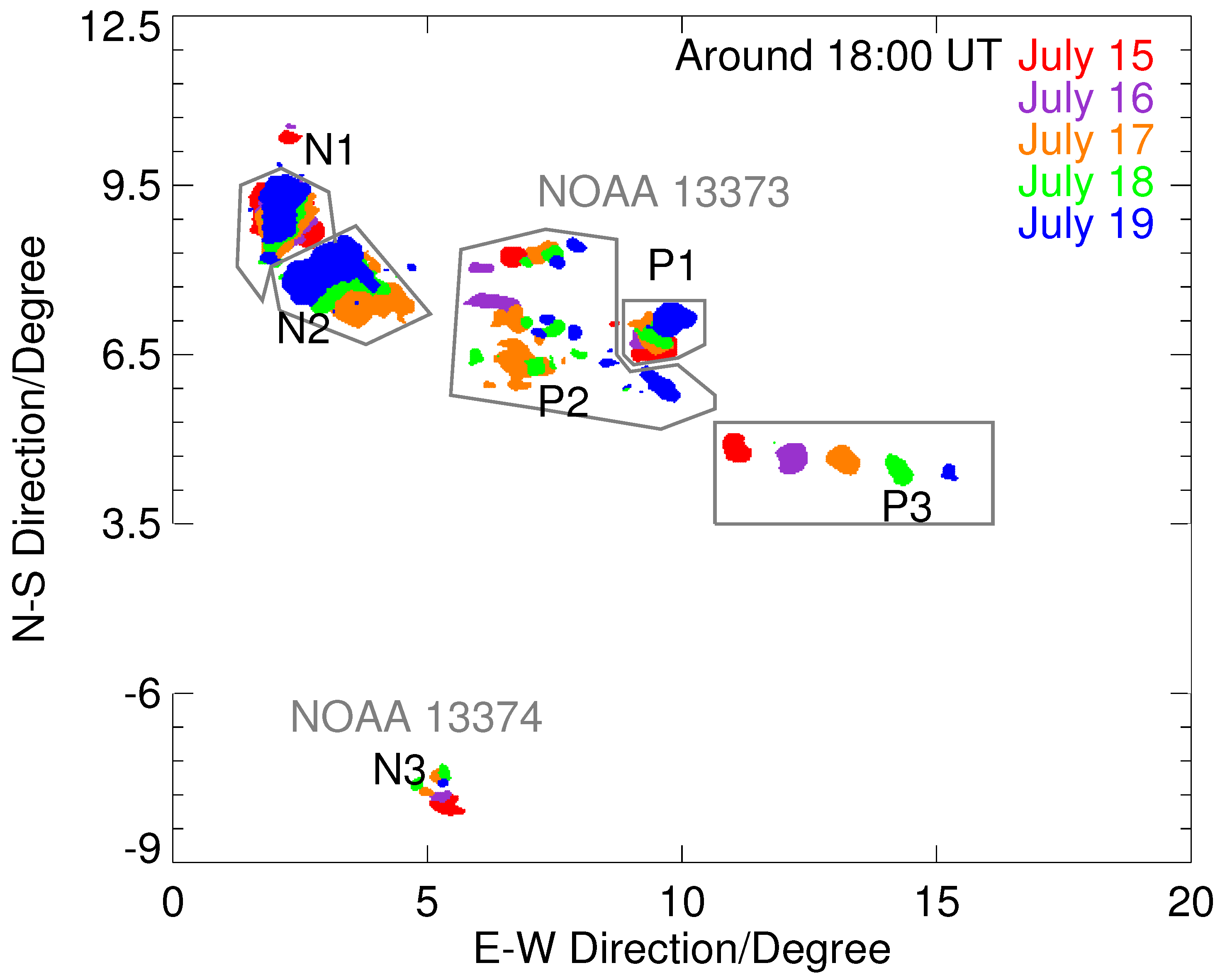
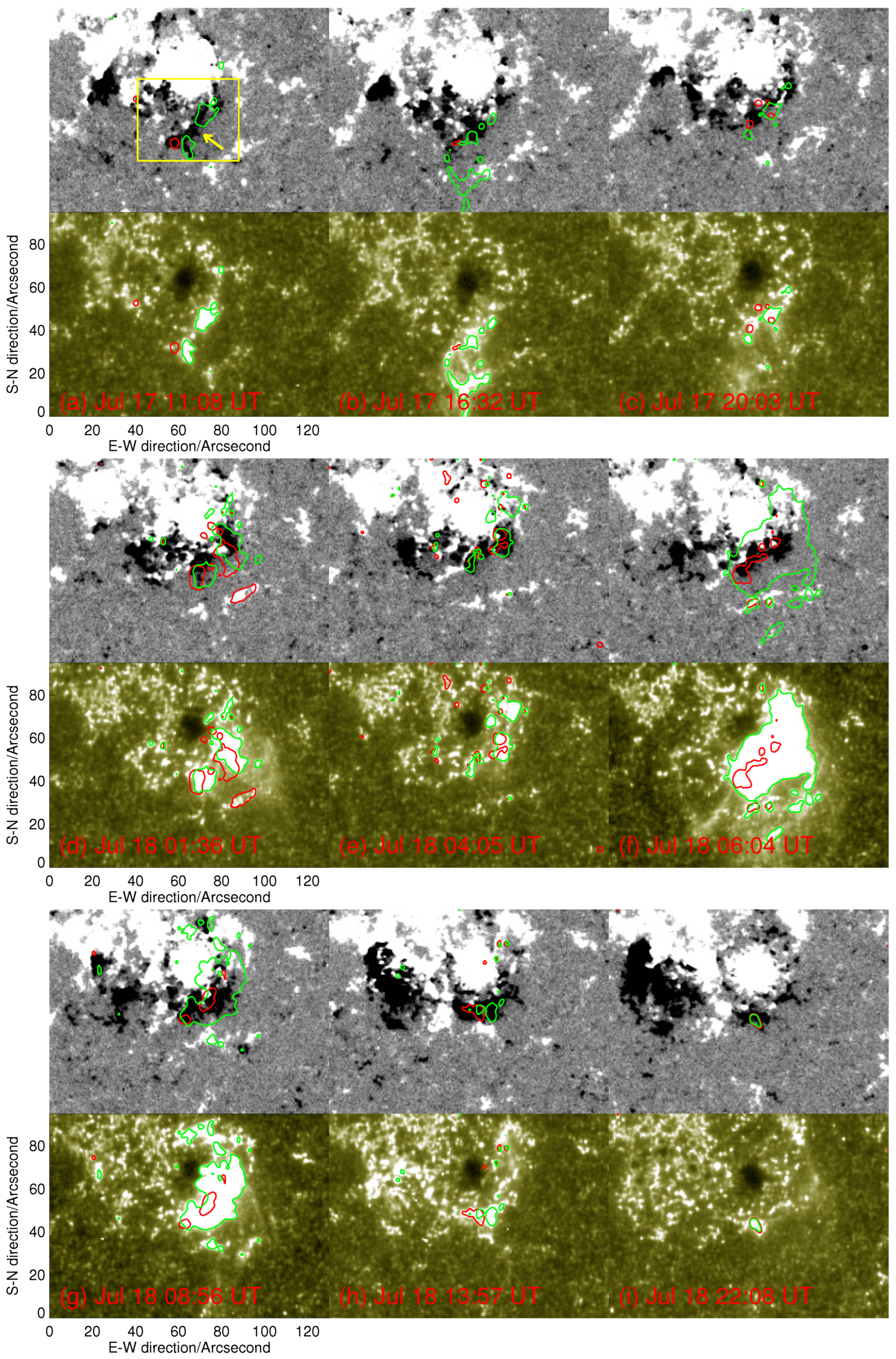
3.1. Long Term Evolution of Active Regions

NOAA 13373 and NOAA 13374 appeared at the solar east limb on 14 July 2023 and rotated to the backside of the Sun after 25 July 2023. The recurring MFR frequently appears from 16 July to 19 July. The temporal evolution of both active regions during these period, which was recorded by FMG, is shown in Figure 1. The sunspot umbra, with its brightness less than 0.65 times the quiet region in the continuum image around 18:00 UT on each day, is labeled with colors corresponding to different dates. It is worth to noting that, in order to save space, the Y-axis is not continuous. As shown in the figure, NOAA 13373 in the Northern Hemisphere was a β-type active region on 15 July, consisting of a dipole polarity configuration with P1 and N1. Both remained stable during its solar disk passage and appeared as different color patches placed on top of Figure 1. A new dipole of P2 and N2 emerged between P1 and N1 around 17 July. After emergence, P2 moves toward the southwestern direction, and N2 moves toward the northeastern direction. In Figure 1, both appear as different color patches slipping away from one another. There is an isolated sunspot labeled as P3, which was about 2.7 × 10⁴ km away from its nearby sunspot P1 on 16 July. This length is calculated based on the distance between the centroids of both P3 and P1. P3 moved toward the western direction at almost a consistent velocity of 0.13 ± 0.01 km/s from 15 July to 19 July. On 19 July, the distance between P3 and P1 was about 6.6 × 10⁴ km. The NOAA 13374 appears as a small sunspot in the continuum images. In contrast, in the HMI magnetogram, it is a decaying β-type region, with the following sunspot disappearing; we labeled this as N3. Its umbra, with its brightness less than 0.65 times the quiet region in the continuum, was composed of a small region on 15 July and 16 and two regions on the following days of 17 July and 18 July. As shown in Figure 1, N3 moves toward the eastern direction slowly. Its proper motion was about 0.02 km/s on 16 July. Since it fragmented into two pieces on the following days, the specific value of the proper motion is hard to calculate. Moreover, the proper motion of P3 and N3 during solar disk passage suggests that they may be the footprints of an emerging large-scale coronal structure, with two foot-points moving in opposite directions. In the following section, we present the recurrent MFR, which was recorded by EUV observations, with two footpoints rooted in P3 and N3. The two observational phenomena corroborate each other.

Figure 2 shows an example of the typical magnetic properties of NOAA 13373 and 13374 on 18 July 2023 at 13:24 UT. Figure 2a,b are the vector magnetograms. The background is the line-of-sight magnetic field, with white denoting positive and black denoting negative. The green arrows represent the transverse magnetic field, with its length being in direct proportion to the value of the transverse magnetic field. The letters marked in Figure 2 are the same as those in Figure 1. As shown in Figure 2a, P3 is isolated from the main part of NOAA 13373. Around P3, there are MMFs, with negative (opposite) polarities converging at its south. In Figure 2b, N3 is shown with an environmental decaying area. Around N3, there are also MMFs with almost the same polarities.

Based on vector magnetic field observation, the vertical current density can be calculated through $J_z={\displaystyle \frac{1}{{\mu }_0}}({\displaystyle \frac{\partial B_y}{\partial x}}-{\displaystyle \frac{\partial B_x}{\partial y}})$. Meanwhile, the z-component of the current helicity $H_c$, which describes the chirality of the solar magnetic field, can be calculated by $H_c=B_z{J}_z$. As discussed in [28], the error of $J_z$ is estimated to be of the order of 0.02 A m⁻². The corresponding error for $H_c$ is around 0.01 G² m⁻¹. The $J_z$ map is shown in the second row in Figure 2. We find that $J_z$ is almost evenly distributed over NOAA 13373. In particular, there is no strong current density area that can be found along PILs. Many previous studies stated that strong current densities along the PILs indicate the area where magnetic free energy is mainly stored (e.g., [29]) and where magnetic reconnection probably occurs (e.g., [30,31]). This is consistent with the behavior of NOAA 13373, which only host several C-class flares during its solar disk passage. Around P3 and N3, there is also no strong current density area.

The $H_c$ map is shown in the third row of Figure 2. The $H_c$ values for NOAA 13373 and NOAA 13374 are about −882 G² m⁻¹ and 139 G² m⁻¹, respectively. Both active regions follow the helicity hemispherical sign rule. The $H_c$ values for P3 and N3, as circled by the white boxes in Figure 2c,d is about −45 G² m⁻¹ and −19 G² m⁻¹, respectively. The same chirality of P3 and N3 is consistent with our expectation that, for an MFR, both footpoints should have the same chirality.

3.2. Recurrence of the MFR

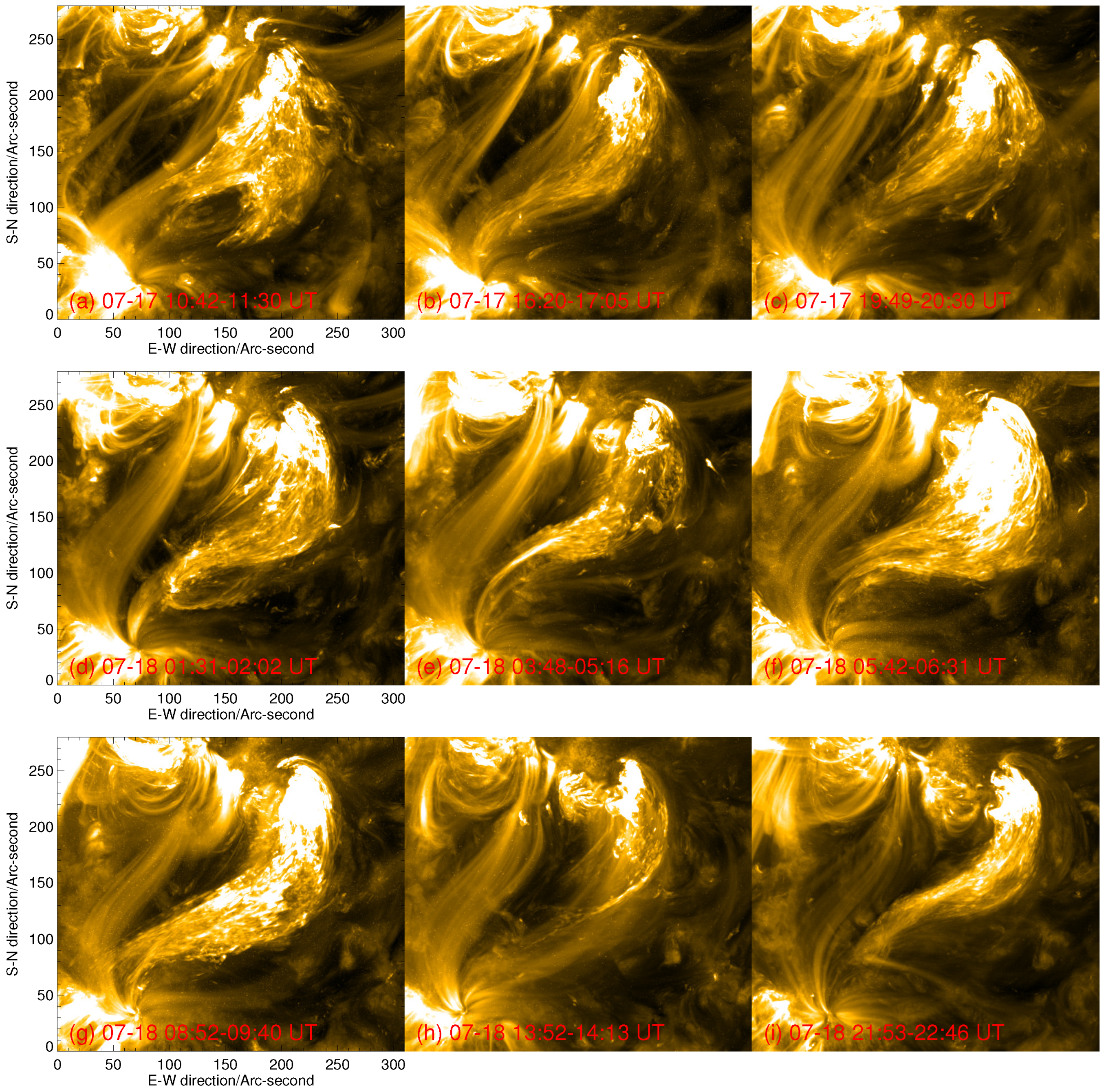
3.2.1. Overview of the Recurrence of the MFR

Figure 3 shows the morphology of NOAA 13373 and NOAA 13374 during their solar disk center passage on 18 July 2023 at around 22:12 UT. Figure 3a shows the continuum image, and Figure 3b shows the longitudinal magnetic field. Green contours outline areas where the brightness is ≤0.65 times the average intensity of the quiet Sun in the continuum image. During their solar disk passage, solar activities, which appear as UV/EUV brightening around P3, occur frequently. The counterpart of UV/EUV brightening observed by AIA EUV wavelengths can be classified into two types. Figure 3c,d show two examples of activities that appear as EUV brightening on 18 July at around 19:31 UT and 22:12 UT in AIA 171 Å image, respectively. For the event that occurred at around 19:31 UT, as shown in Figure 3c, EUV brightening is associated with a jet-like structure with a narrow field angle (indicated by red arrows). For the event that occurred at around 22:12 UT, as shown in Figure 3d, we have identified a large MFR that spans across two active regions in the northern and southern hemispheres of the Sun. Among them, the active region in the northern hemisphere gradually grew and transformed into a new floating region. Accompanying the slow rise and extension of the active region, a transequatorial MFR (indicated by red arrows) connected P3 and N3 appeared. This is a typical example of an MFR, with braided fine structures within their body clearly observed. The MFR becomes visible for about a few minutes or a few tens of minutes. During solar disk passage, both activities take place more than forty times. In this study, we will focus on the second type, with nine events selected. The detailed information of these events is listed in

Table 1. Event list.

Num	Date	Tstart	Tpeak	Tend	GOES 1	DN 2	MMF 3
01	07-17	10:42	11:09	11:30	No	2.4	N
02	07-17	16:20	16:32	17:05	No	3.4	N
03	07-17	19:49	20:03	20:30	No	2.9	P&N
04	07-18	01:31	01:37	02:02	No	6.0	P&N
05	07-18	03:48	04:05	05:16	No	1.7	P&N
06	07-18	05:42	06:08	06:31	B5.8	31.0	P&N
07	07-18	08:52	09:04	09:40	C4.4	12.8	P&N
08	07-18	13:52	13:59	14:13	No	1.6	N
09	07-18	21:53	22:08	22:46	No	0.6	N

¹ The maximum GOES flux intensity during the time period from the event’s start to the event’s end if the GOES flux has a corresponding peak with the EUV flux. ² Total detected number in 1600 Å around the maximum time subtracted by the initial time; the unit is 10⁵. ³ N means that the initial brightening only occurred in the negative polarity, and P&N means that the initial brightening occurred in both negative and positive polarities;

.

The blue contour in Figure 3d outlines a large area that involves the profile of both types of activities. By obtaining this contour, we create an image in which the value of each pixel is the maximum value during the long period from 16 July 00:00 UT to 22 July 00:00 UT. The profile is outlined by hand along the bright area and overlay on Figure 3d. Within the profile, using images with a temporal resolution of 1 min and along the Y direction, a time–distance plot is obtained and shown in Figure 3e. In this diagram, each pixel along the Y direction is the maximum value of the pixel with the same Y value, and the values along the X direction within the profile are outlined by a blue contour. In Figure 3e, the X-axis represents time, starting on 16 July 00:00 UT and ending on 20 July 00:00 UT. In Figure 3e, each thin brightening line represents one event, with the length representing the part of the visible MFR or the distance that the jet traveled. The short green lines indicate the events selected in this study. The short blue lines mark the times corresponding to the images shown in Figure 3c,d. Figure 3f is the time–distance diagram along the white line, as shown in Figure 3d. The thin brightening line shows the expanded body of the MFR. As shown in this image, the MFR did not erupt during the long-term period. Figure 3g,h show the AIA flux evolution around P3 and N3, as circled by the black and red boxes in Figure 3b. The 304, 171, and 94 Å wavelengths are represented by green, black, and blue curves, respectively. The red curve in Figure 3g shows the GOES flux in the 1–8 Å energy band. During the period from 16 July 00:00 UT to 20 July 00:00 UT, nine C-class flares occurred in NOAA 13373, which are indicated by black lines. The green lines are the same as those shown in Figure 3d. As shown by the black and green lines, only two of them are located closely. One is the third event, and the other is the seventh event, as labeled in Table 1. By looking though the temporal evolution of the AIA images, we observe that the first flare occurred around the core region of NOAA 13373, and the second flare is associated with the active event studied here. By plotting the GOES flux variation in the 1–8 Å energy band and the AIA flux variation in 171 Å together, we also find that, for the first flare, the temporal variations in both fluxes are not consistent. We plotted the same flux variation image for all events. We found that only two events had the same trends in the variations of the GOES flux and AIA flux curves. The maximum flux intensities for these two events are labeled in Table 1. One corresponds to a B5.8 flare, and the other corresponds to a C4.4 flare. This observational evidence means that the appearance of the MFR is triggered by small activities. Meanwhile, as shown in Figure 3f, the flux variation associated with the appearance of the MFR can be identified in both cool (304 and 171 Å) and hot (94 Å) wavelengths. For NOAA 13374, no flare greater than C-class was recorded. The AIA flux variation and the appearance of the MFR are uncorrelated. In the following section, we will focus on the magnetic field variations in P3.

Figure 4 is the maximum image value for all events listed in Table 1. All MFRs outline a similar profile with a reversed S-shape structure, with braided features inside. We will present typical examples to illustrate the dynamic evolution of the recurrent MFR.

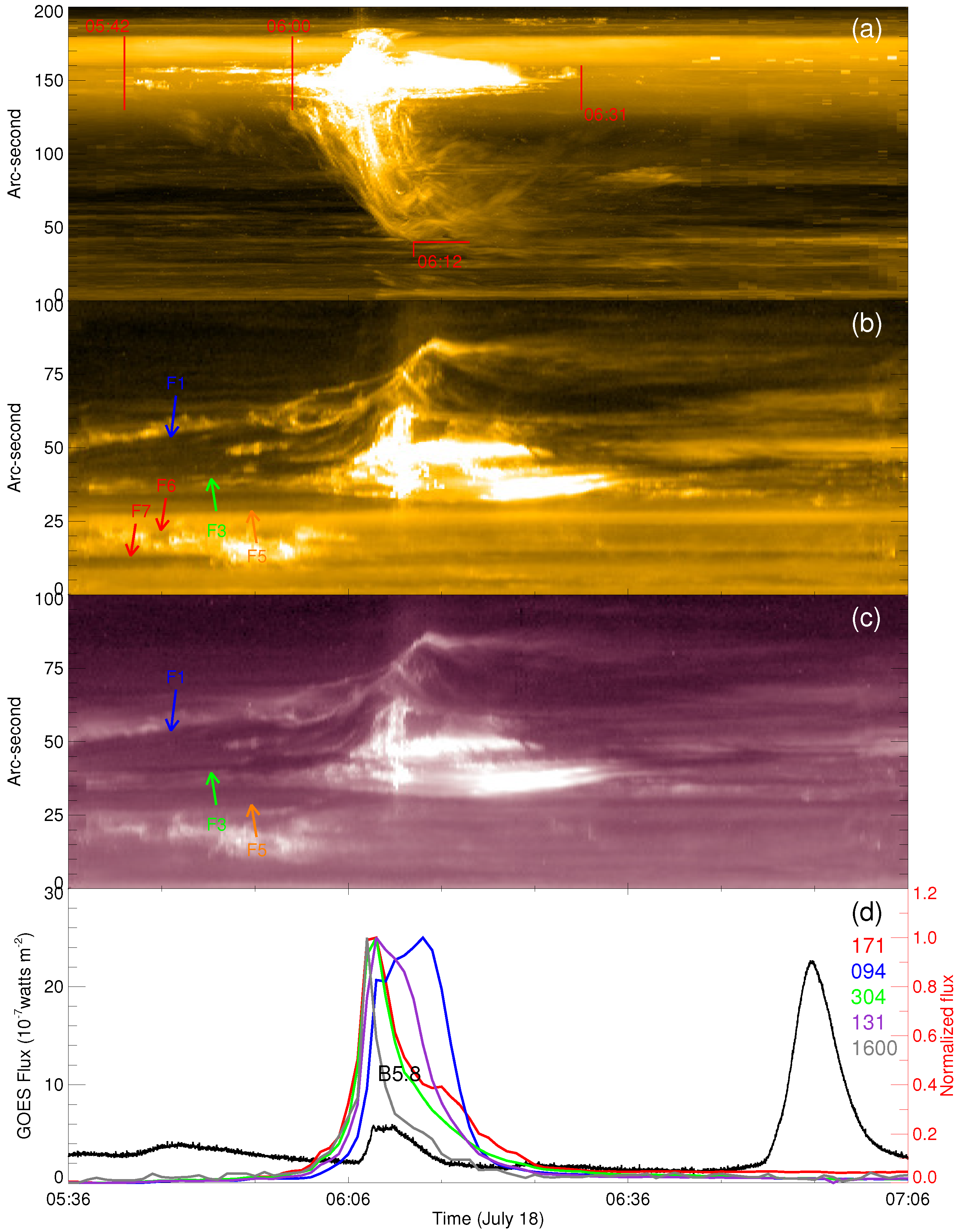
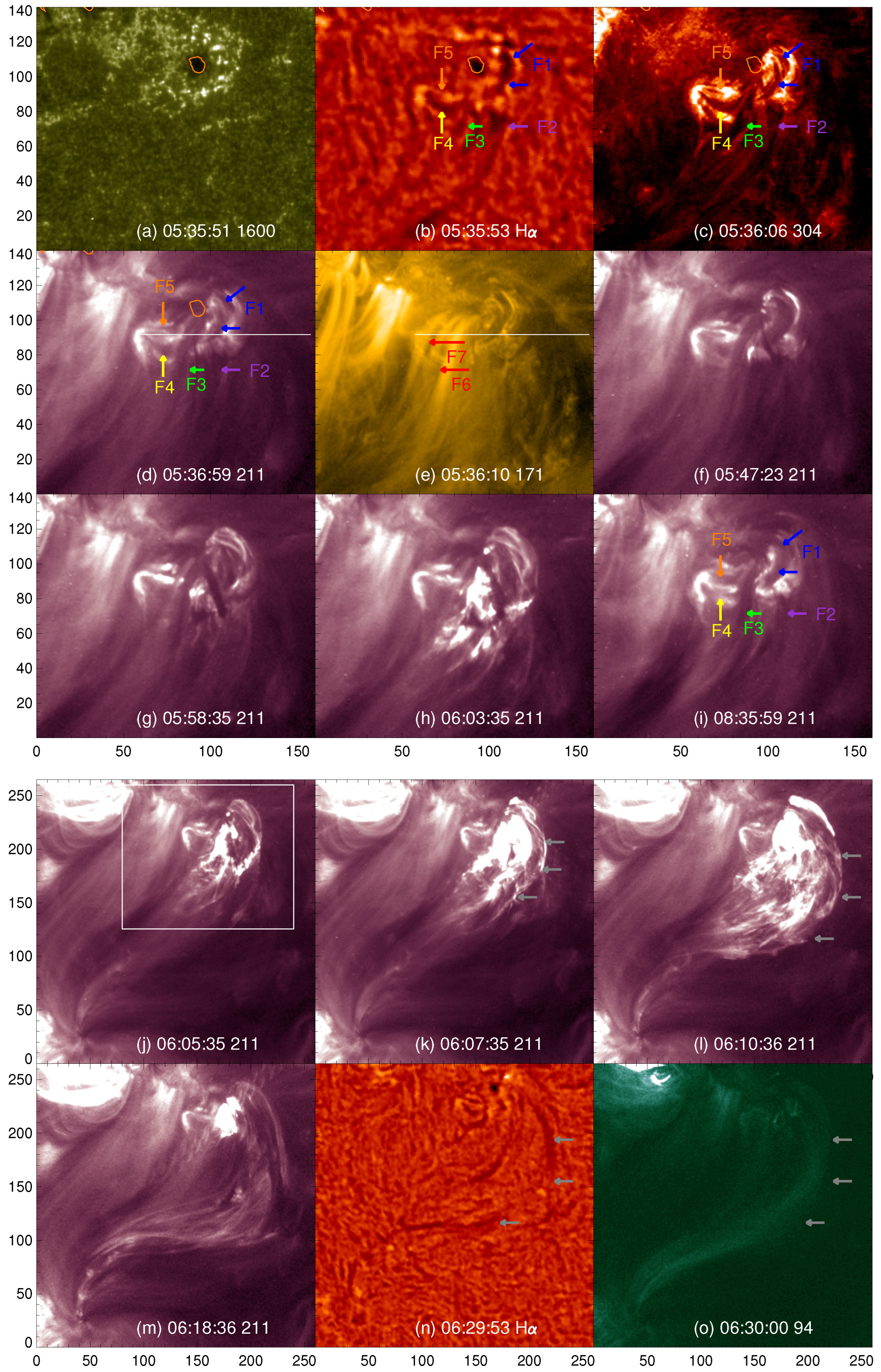
3.2.2. Jul 18 05:42–06:31

Figure 5 shows an overview of the dynamic evolution of the MFR’s appearance during the period from 18 July 05:42 UT to 06:31 UT. Figure 6 shows the morphological evolution at selected time in multi-wavelengths to illustrate the details of the dynamic evolution. This is the most powerful event, as shown in Figure 4f, and the MFR appears with its widest and nearly complete body. Figure 5a shows an expanded small portion along the time axis of Figure 3 during the period from 18 July 05:36 UT to 07:06 UT. This image shows the temporal evolution of local brightening and the MFR that gradually appeared at 211 and 171 Å due to heating and perturbations. Figure 5b,c show the time–distance images along the white line shown in Figure 6d,e. Both images show the temporal evolution of filaments located around P3. Figure 5d shows the temporal profile of the normalized flux of the AIA 171 (red), 94(blue), 304 (green), 131 Å (purple), and 1600 Å observations. These curves show that the activities result in an increase in flux intensity for all wavelengths. The black curve represents the flux of GOES in the 1–8 Å wavelength range. As shown in Figure 5d, even though it is small, the GOES flux increases with the maximum flux intensity, reaching the level of B5.8. As shown in Figure 5a–c, local brightening is blocked by the upper filaments, with light only shining through gaps in the filaments. The active process shown in Figure 5a is relatively simple. The red vertical lines mark the time notes. As shown in Figure 5a, initial brightening in the lower atmosphere starts at around 05:42 UT near the north leg. The initial brightening is sheltered from the upper filament, which appears as a dark narrow stripe. The sudden brightening phenomena that appeared in the EUV wavelengths are generally believed to be caused by magnetic reconnection. The main energy release occurs at around 06:00 UT. This is associated with the rapid increase in the flux intensities in all AIA wavelengths and the rise and expansion of the upper filament. The extended filament is mixed with dark and bright features. In association with the filament activities, the MFR hosting the filament reveals itself bit by bit. At around 06:12 UT, the MFR exhibits its longest body, and then, the filament material is drained back to its north leg. In the lower atmosphere, EUV brightening disappears at around 06:31 UT, which is a signal for the ending of these events.

The detail temporal evolution is shown in Figure 6. It is worth noting that the FOV of the first three rows is outlined by the white box in Figure 6j. Figure 6a shows the AIA 1600 Å image at around 05:35 UT, which is just before the activity. The orange contour circles the area where the brightness is ≤0.7 times the average brightness of the quiet Sun in the 1600 Å image. The same contour is overlaid on the Hα, 304, and 211 Å images in Figure 6b–d to show the positional relationship between P3 and the filaments before eruption. As shown in Figure 6b–e, there are several filaments rooted in the moss area around P3 at different heights. The Hα image shows the profile of the filaments, while the AIA 304 Å image reveals more details of the morphology of the EUV filaments. As shown in Figure 6c, to the west of P3, two dark fibers wind around each other to form filament F1. Around the south footpoint of F1, three filaments extend in different directions. Two large filament structures, F2 and F3, extend to the south. A small filament, F4, appears as with an arch-shaped structure extending toward the east. Another small filament is located at the north of F4.

As shown in Figure 6d, their counterpart in the EUV wavelength can be seen clearly in the cool AIA wavelength at 211 Å. In the 171 Å image, as shown in Figure 6e, only F1 can be identified easily. Meanwhile, two dark features, as indicated by F6 and F7, spans across F3, and they cannot be identified in Figure 6b–d. The 304 and 211 Å band-passes are sensitive to coronal plasma, with peak temperature responses of ~0.05 and ~2 MK, respectively. In contrast, the 171 Å band-pass is sensitive to 0.6 MK. This means that F6 and F7 are structures with a relatively small temperature range.

As shown in Figure 5b,c, the filaments were already in their slow rising phase at around 05:36 UT, with lower atmosphere brightening appearing as bright narrow strips on both sides. A small degree of EUV brightening can be found around the filaments, as shown in Figure 6d–g. As shown in Figure 6h, EUV brightening suddenly became intense. In association with this brightening phenomenon, a large upper filament appeared and began to expand and slow rise. The large filament can be seen more clearly in Figure 6k, as indicated by gray arrows. The twisted structures within this filament can be seen more clearly in Figure 6l, where bright and dark fibers are interwoven. This filament can also be seen in Hα (Figure 6n) and appears as a hot channel in the 94 Å image (Figure 6o). It is worth noting that Figure 6i shows the morphology of the host region around P3 at 08:36 UT. The morphology of the filaments is almost the same as that shown in Figure 6c, which was obtained at around 05:36 UT, just before the activities.

The observations show that EUV brightening under the filaments starts before the rising motion of the filament and the appearance of the MFR. The MFR then becomes visible in association with the expansion of the hosting filament. The slow rise of the MFR is initiated by the energy released from low-atmosphere reconnections rather than from the loss of equilibrium. Ref. [32] presents an observation of two small-scale erupting filaments pushing out an upper filament, ultimately forcing it to erupt. This suggests that the initial kinetic energy of the eruption can be obtained from and transported by other erupting structures. Here, our observations confirm the hypothesis and further point out that if the erupting structure cannot obtain enough energy to reach the escape velocity, it will return to its initial morphology.

All selected events show a similar dynamical evolution of low-atmosphere reconnection below filaments and the transient appearance of the MFR, which occurred around the isolated leading sunspot of NOAA 13373 (P3). The appearance of the MFR is initiated by the the low-atmosphere reconnection. It occurs right below the filament, so its dynamic evolution is not visible. Only UV brightening, recorded by AIA 1600 Å, can indicate the possible site of the energy release area. The energy released by reconnection heated the nearby plasma and then lifted the upper MFR/filament. The disturbed MFR usually appears as gradually extended dark filaments in Hα and cool EUV wavelength observations, and it appears as hot channels in hot EUV wavelength observations. The slow rise and extension of the filament make the MFR visible though the heating of filament materials. During the extension, the filament exhibits alternately shaded and braided fibers in its body, which is a typical morphology of the MFR. The extended filament is then slowly restored to its initial morphology through a transformation and darkening process. Since the low-atmosphere reconnection is obscured by the upper filament, it is hard to determine the ending time. Here, we use the brightening time around P3 to determine the start and end time of each event. Detailed information about the appearance of the MFR can be found in Table 1.

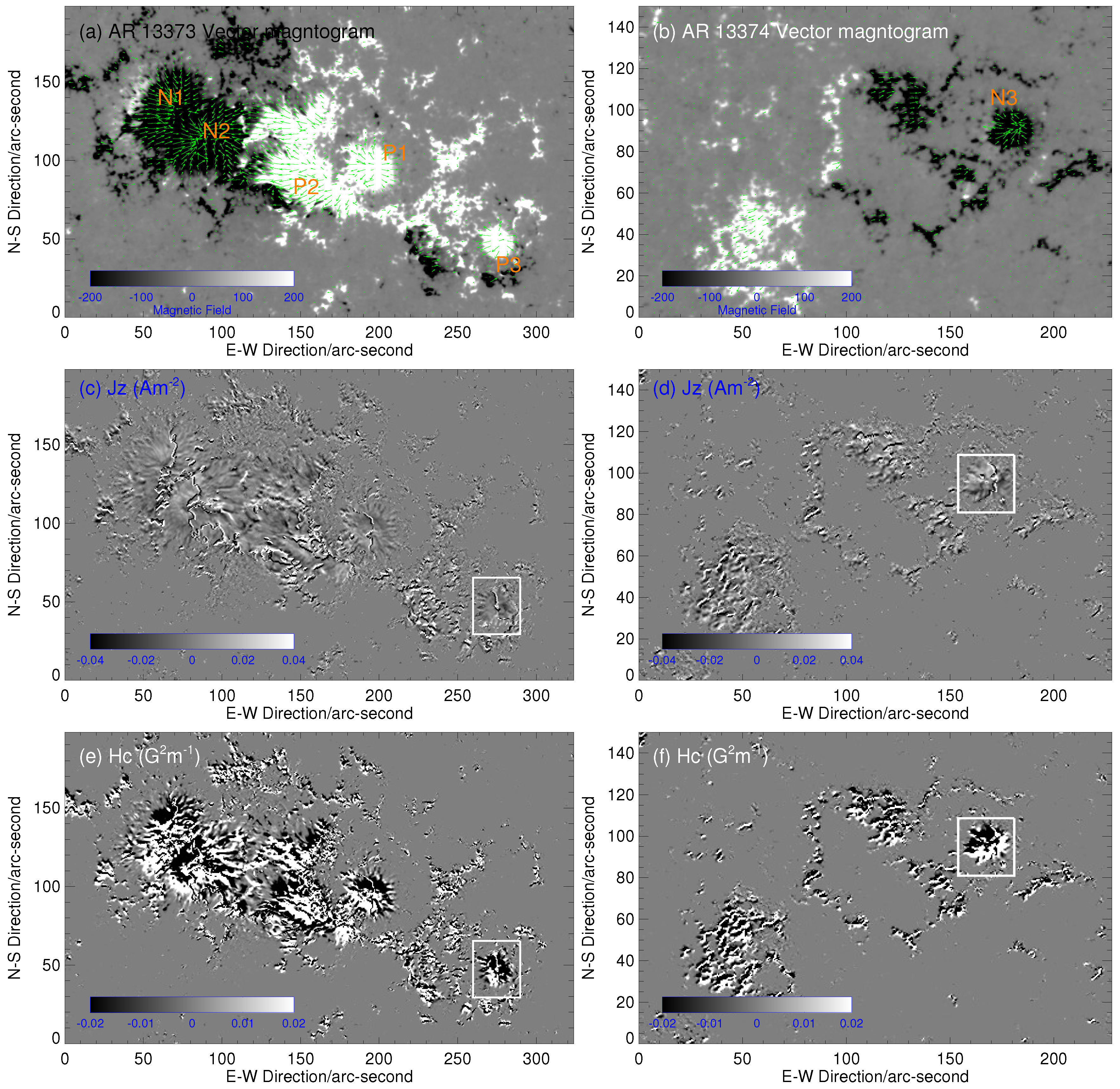
3.3. Magnetic Configuration

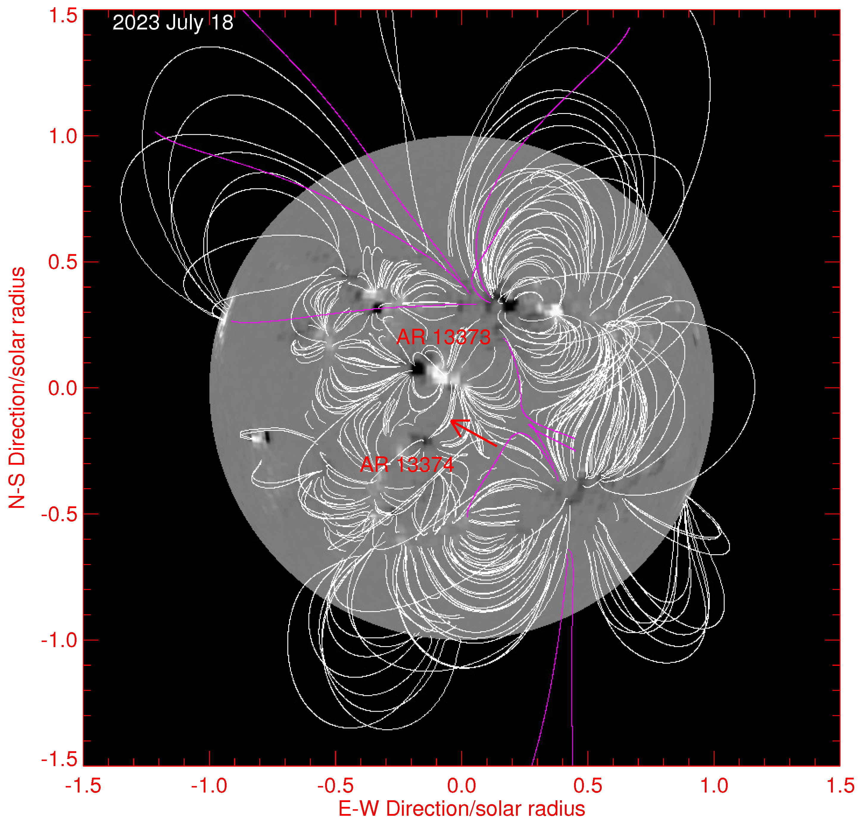
3.3.1. Large-Scale Magnetic Connection

To investigate the magnetic configuration evolution associated with the recurrence of the MFR, we studied the magnetic connection between NOAA 13373 and NOAA 13374 by extrapolating coronal magnetic fields. Potential field extrapolation is the simplest method for obtaining coronal magnetic fields. It only requires a line-of-sight photospheric magnetogram as the boundary condition and is capable of reproducing the basic coronal magnetic field structure, especially for large-scale magnetic connections. We used the standard program of PSFF in SolarSoftWare (SSW) to perform potential field extrapolation [33,34]. The results show that the large-scale MFR connecting NOAA 13373 and NOAA 13374 remained almost the same during the period from 16 July 2023 to 20 July 2023. We show the example for 18 July 2023 in Figure 7. In Figure 7, the units of the X-axis and Y-axis are solar radii. As shown in Figure 7, the transequatorial magnetic structure, which connects P3 in NOAA 13373 and N3 in NOAA 13374, is outlined by a red arrow. Since the coronal magnetic structure is obtained through potential field extrapolation, we should not expect to see twists in the coronal magnetic field, which usually appear in nonlinear force-free extrapolation and are common structures of the MFR, to appear here.

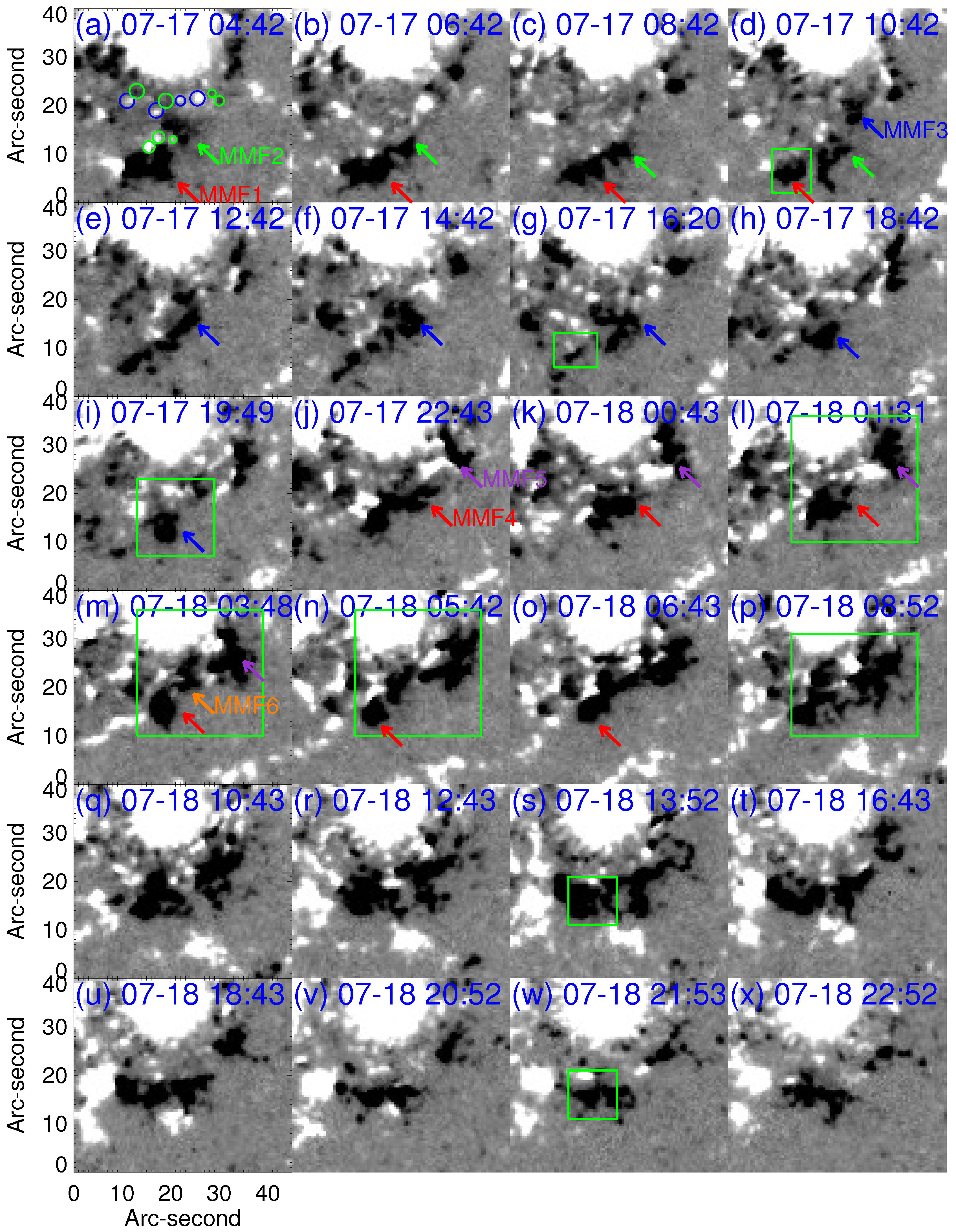
3.3.2. Magnetic Moving Feature Around the Initial Brightening Area

As shown in Figure 5, the event initially occurred around the northern footpoint of the MFR, which is rooted around sunspot P3 in AR 13373. The most remarkable evolutionary feature of P3 is the MMFs, which appear as small isolated single or dipole magnetic elements around the outer penumbra of P3.

Figure 8 shows the AIA image at 1600 Å around the maximum time of each activity (top image on each line) and the simultaneous line-of-sight magnetograms at the photosphere (bottom image on each line). The brightening areas are labeled by different images, which are obtained by subtracting the previous image (about several minutes before the initial brightening) from the initial brightening image or the maximum brightening image. The threshold value of the contour is 100 detection instances in different images. In Figure 8, the EUV brightening around the initial and peak times is outlined by red and green contours, respectively. As shown in Figure 8, the initial UV brightening in AIA 1600 Å appears as compact brightening areas around the edge of P3, where the MMFs occurred. For most events, except for the sixth and seventh events shown in Figure 8f,g, the UV brightening area at its maximum is also a compact bright point, similarly to the initial brightening, albeit with a slightly larger area or a minor shift in position. Particularly for the ninth event, the brightening area is almost identical at both the initial and maximum times, as shown in Figure 8i. In contrast, for the sixth and seventh events, the UV brightening area at its maximum appears as an extending area. UV brightening is consistent with the information shown in Table 1, where only the sixth and seventh events exhibit flux enhancements in the X-ray energy band of 1–8 Å.

As shown in Figure 8, all events almost occur at around the same location, where the new MMFs are squeezed by pre-existing negative MMFs. The magnetic field’s evolution is shown in Figure 9. To display the rapidly moving sunspot P3 within a small box over a long time period, the proper motion of P3 is corrected by placing the centroid of P3 at the same position throughout the sequence. It is also worth noting that the time intervals between the images in this figure are not uniform. The magnetic field maps shown in this figure correspond to the initial brightening time for each event, rather than showing maps around different times. As shown in Figure 9, the significant evolutionary characteristic of P3 is the continuous emergence of MMFs at its edge. We circle some MMFs (not all) in Figure 9a as examples. During outward motions, some negative MMFs encounter the surrounding positive-polarity structures, and they are squeezed and undergo cancellation. However, another part of the negative MMFs continuously merges with MMFs of the same polarity to form larger negative MMFs. These larger negative MMFs keep merging with incoming MMFs of the same polarity and persist for a longer period of time. In the evolution process shown in the figure, such a negative-polarity structure always existed. As shown in Figure 9a, two large negative MMFs (MMF1 and MMF2) are indicated by red and green arrows, respectively. During the time period shown in Figure 9, both MMF1 and MMF2 are in their decaying phase. As shown in Figure 9a–g, many small positive MMFs are canceled. As circled by the green box in Figure 9d,g, the initial brightening area of the first and second events is co-spatial with respect to MMF1. Meanwhile, during their decaying phase, another negative polarity (MMF3), indicated by blue arrows in Figure 9d–i, forms. MMF3 merges with MMF2 and then fragments from MMF2 and cancels the surrounding positive polarities. The initial area of the third event, as circled by the green box in Figure 9i, is co-spatial with respect to the decaying phase of the MMF3. As indicated by the red arrow in Figure 9j–o, MMF4 merges with MMF3. MMF5, indicated by a purple arrow, forms at the northwest of MM4, with a positive polarity in between. This positive polarity disappears due to continuous cancellation, with negative MMFs moving towards it. Subsequently, a new negative-polarity MMF6, indicated by the orange arrow in Figure 9m, forms. The initial brightening areas from the fourth to seventh events are co-spatial with respect to the dynamic evolution of MMF4, MMF5, and MMF6. The last two events occur during the decay phase of these MMFs.

As shown in Figure 9, these long-lived MMFs, as labeled in this figure, underwent a complex evolution process. They continuously interacted with other MMFs that moved towards them, merging with those of the same polarity and canceling out those of opposite polarities. These processes of cancellation and merging occurred throughout their entire evolution. As shown in Figure 8 and listed in Table 1, some initial UV brightening areas are co-spatial with respect to the magnetic cancellation area between the new MMF and the pre-existing magnetic features, while others are co-spatial with respect to unipolarity. It is believed that UV brightening occurs due to the particles propagating along the reconnection-formed field lines to the lower atmosphere, heating the plasma there through Coulomb collisions (e.g., [35]). This represents the magnetic field that is involved in the reconnection process. These observational results are consistent with those reported by the authors of [36], who noted that the relationship between magnetic field variations and solar activity initiation is complex. The appearance of flux emergence or cancellation alone is not unique for the initiation of solar activities.

4. Conclusions

In this study, we presented observational evidence for the recurring pre-existing transequatorial MFRs during the period from 17 July 2023 to 19 July 2023, and we inferred that the MMFs may play a key role in energy storage and trigger the mechanism of the small activities that result in the appearance of the MFR. The transequatorial MFR connects the leading sunspot P3 in NOAA 13373 (in the Northern hemisphere) and the leading sunspot N3 in NOAA 13374 (in the Southern hemisphere). The activity begins with EUV brightening, which is observed by AIA at all wavelengths occurring in the south of P3, where there are MMFs everywhere. The single or bipolar MMFs form around the boundary of P3 and move outward. Except for those that cancel the nearby positive polarity, most negative polarities merge. During the continuous cancellation of the surrounding positive MMFs, new negative MMFs also keep merging in. As a result, the negative MMFs persist in this region for an extended period, and all initial activities occurred here. They first appear as EUV brightening phenomena, which can only be seen through the gaps in the filaments from the EUV observations. This suggests that small-scale reconnection occurs in the lower atmosphere beneath the filament structures. It converts magnetic energy into heat and kinetic energy in the corona. The small filaments located above the EUV brightening area undergo slow rising and expansion processes. At the same time, a large magnetic structure, which appears as twisted filaments in cool AIA wavelengths and hot channels in hot AIA wavelength, appears. This structure exhibits fine structures with alternately shaded and braided fibers in its body during the expansion phase, which is a typical morphology of the MFR. We suggest that this structure is the pre-existing MFR. It rises and expands slowly and then returns to its starting position. Ultimately, all structures return to their pre-activity state.

References

1. Chase, L.F.; Jordan, W.C.; Perez, J.D.; Johnston, R.R. X-ray Spectrum of a Laser-produced Iron Plasma. Phys. Rev. A 1976, 13, 1497. [Google Scholar] [CrossRef]
2. Stewart, R.T.; Vorpahl, J. Radio and soft X-ray evidence for dense non-potential magnetic flux tubes in the solar system. Sol. Phys. 1977, 55, 111. [Google Scholar] [CrossRef]
3. Tsuneta, S. Structure and Dynamics of Magnetic Reconnection in a Solar Flare. Astrophys. J. 1996, 456, 840. [Google Scholar] [CrossRef]
4. Bagalá, L.G.; Mandrini, C.H.; Rovira, M.G.; Démoulin, P. Magnetic reconnection: A common origin for flares and AR interconnecting arcs. Astron. Astrophys. 2000, 363, 779. [Google Scholar]
5. Wang, H.; Chae, J.; Yurchyshyn, V.; Yang, G.; Steinegger, M.; Goode, P. Inter-Active Region Connection of Sympathetic Flaring on 2000 February 17. Astrophys. J. 2001, 559, 1171. [Google Scholar] [CrossRef]
6. Guité, L.-S.; Strugarek, A.; Charbonneau, P. Flaring together: A preferred angular separation between sympathetic flares on the Sun. Astron. Astrophys. 2025, 694, A74. [Google Scholar] [CrossRef]
7. Zhang, Q. Circular-ribbon flares and the related activities. Rev. Mod. Plasma Phys. 2024, 8, 7. [Google Scholar] [CrossRef]
8. Jiang, Y.; Yang, J.; Hong, J.; Bi, Y.; Zheng, R. Sympathetic Filament Eruptions Connected by Coronal Dimmings. Astrophys. J. 2011, 738, 179. [Google Scholar] [CrossRef]
9. Khan, J.I.; Hudson, H.S. Homologous sudden disappearances of transequatorial interconnecting loops in the solar corona. Geophys. Res. Lett. 2000, 27, 1083. [Google Scholar] [CrossRef]
10. Yang, S.B.; Büchner, J.; Zhang, H.Q. Magnetic Helicity Exchange Between Neighboring Active Regions. Astrophys. J. 2009, 695, L25. [Google Scholar] [CrossRef]
11. Zhou, G.P.; Wang, J.X.; Wang, Y.M.; Zhang, Y.Z. Quasi-Simultaneous Flux Emergence in the Events of October & November 2003. Sol. Phys. 2007, 244, 13. [Google Scholar]
12. Zhou, G.P.; Tan, C.M.; Su, Y.N.; Shen, C.L.; Tan, B.L.; Jin, C.L.; Wang, J.X. Multiple Magnetic Reconnections Driven by a Large-scale Magnetic Flux Rope. Astrophys. J. 2019, 873, 23. [Google Scholar] [CrossRef]
13. Zhou, G.P.; Wang, J.X.; Zhang, J. Large-scale source regions of earth-directed coronal mass ejections. Astron. Astrophys. 2006, 445, 1133. [Google Scholar] [CrossRef]
14. Sheeley, N.R. The Evolution of the Photoshperic Network. Sol. Phys. 1969, 9, 347. [Google Scholar] [CrossRef]
15. Pariat, E.; Antiochos, S.K.; DeVore, C.R. Three-dimensional Modeling of Quasi-homologous Solar Jets. Astrophys. J. 2010, 714, 1762. [Google Scholar] [CrossRef]
16. Yang, L.; He, J.; Peter, H.; Tu, C.; Zhang, L.; Feng, X.; Zhang, S. Numerical Simulations of Chromospheric Anemone Jets Associated with Moving Magnetic Features. Astrophys. J. 2013, 777, 16. [Google Scholar] [CrossRef]
17. Mou, C.; Huang, Z.; Xia, L.; Madjarska, M.S.; Li, B.; Fu, H.; Jiao, F.; Hou, Z. Magnetic Flux Supplement to Coronal Bright Points. Astrophys. J. 2016, 818, 9. [Google Scholar] [CrossRef]
18. Wyper, P.F.; DeVore, C.R. Simulations of Solar Jets Confined by Coronal Loops. Astrophys. J. 2016, 820, 777. [Google Scholar] [CrossRef]
19. Wei, H.; Huang, Z.; Li, C.; Hou, Z.; Qiu, Y.; Fu, H.; Bai, X.; Xia, L. Internal Activities in a Solar Filament and Heating in Its Threads. Astrophys. J. 2023, 958, 116. [Google Scholar] [CrossRef]
20. Chen, J.; Su, J.; Yin, Z.; Priya, T.G.; Zhang, H.; Liu, J.; Xu, H.; Yu, S. Recurrent Solar Jets Induced by a Satellite Spot and Moving Magnetic Features. Astrophys. J. 2015, 815, 71. [Google Scholar] [CrossRef]
21. Zhang, J.; Wang, J. Are Homologous Flare-Coronal Mass Ejection Events Triggered by Moving Magnetic Features? Astrophys. J. 2002, 566, L117. [Google Scholar] [CrossRef]
22. Deng, Y.-Y.; Zhang, H.-Y.; Yang, J.-F.; Li, F.; Lin, J.-B.; Hou, J.-F.; Wu, Z.; Song, Q.; Duan, W.; Bai, X.-Y.; et al. Design of the Full-disk MagnetoGraph (FMG) onboard the ASO-S. Res. Astron. Astrophys. 2019, 19, 157. [Google Scholar] [CrossRef]
23. Gan, W.; Zhu, C.; Deng, Y.; Zhang, Z.; Chen, B.; Huang, Y.; Deng, L.; Wu, H.; Zhang, H.; Li, H.; et al. The Advanced Space-Based Solar Observatory (ASO-S). Sol. Phys. 2023, 298, 68. [Google Scholar] [CrossRef]
24. Pesnell, W.D.; Thompson, B.J.; Chamberlin, P.C. The Solar Dynamics Observatory (SDO); Springer: Greer, SC, USA, 2012; Volume 275, p. 3. [Google Scholar]
25. Lemen, J.R.; Title, A.M.; Akin, D.J.; Boerner, P.F.; Chou, C.; Drake, J.F.; Duncan, D.W.; Edwards, C.G.; Friedlaender, F.M.; Heyman, G.F.; et al. The Atmospheric Imaging Assembly (AIA) on the Solar Dynamics Observatory (SDO). Sol. Phys. 2012, 275, 17. [Google Scholar] [CrossRef]
26. Schou, J.; Scherrer, P.H.; Bush, R.I.; Wachter, R.; Couvidat, S.; Rabello-Soares, M.C.; Bogart, R.S.; Hoeksema, J.T.; Liu, Y.; Duvall, T.L., Jr.; et al. Design and Ground Calibration of the Helioseismic and Magnetic Imager (HMI) Instrument on the Solar Dynamics Observatory (SDO). Sol. Phys. 2012, 275, 229. [Google Scholar] [CrossRef]
27. Zhang, H.-Q.; Wang, D.-G.; Deng, Y.-Y.; Hu, K.-L.; Su, J.-T.; Lin, J.-B.; Lin, G.-H.; Yang, S.-M.; Mao, W.-J.; Wang, Y.-N.; et al. Solar Magnetism and the Activity Telescope at HSOS. Chin. J. Astron. Astrophys. 2007, 7, 281. [Google Scholar] [CrossRef]
28. Cheng, X.; Ding, M.D. The characteristics of the footpoints of solar magnetic flux ropes during eruptions. Astrophys. J. Suppl. Ser. 2016, 225, 16. [Google Scholar] [CrossRef]
29. Sun, X.; Hoeksema, J.T.; Liu, Y.; Wiegelmann, T.; Hayashi, K.; Chen, Q.; Thalmann, J. Evolution of Magnetic Field and Energy in a Major Eruptive Active Region Based on SDO/HMI Observation. Astrophys. J. 2012, 748, 77. [Google Scholar] [CrossRef]
30. Cheng, X.; Ding, M.D.; Zhang, J.; Sun, X.D.; Guo, Y.; Wang, Y.M.; Kliem, B.; Deng, Y.Y. Formation of a Double-decker Magnetic Flux Rope in the Sigmoidal Solar Active Region 11520. Astrophys. J. 2014, 789, 93. [Google Scholar] [CrossRef]
31. Vemareddy, P.; Zhang, J. Initiation and Eruption Process of Magnetic Flux Rope from Solar Active Region NOAA 11719 to Earth-directed CME. Astrophys. J. 2014, 797, 80. [Google Scholar] [CrossRef]
32. Song, Y.; Su, J.; Zhang, Q.; Zhang, M.; Deng, Y.; Bai, X.; Liu, S.; Yang, X.; Chen, J.; Xu, H.; et al. Observation of a Large-Scale Filament Eruption Initiated by Two Small-Scale Erupting Filaments Pushing Out from Below. Sol. Phy. 2024, 299, 85. [Google Scholar] [CrossRef]
33. Schrijver, C.J. Simulations of the Photospheric Magnetic Activity and Outer Atmospheric Radiative Losses of Cool Stars Based on Characteristics of the Solar Magnetic Field. Astrophys. J. 2001, 547, 475. [Google Scholar] [CrossRef]
34. Schrijver, C.J.; De Rosa, M.L. Photospheric and heliospheric magnetic fields. Sol. Phys. 2003, 212, 165. [Google Scholar] [CrossRef]
35. Tian, H.; Chen, N.-H. Multi-episode Chromospheric Evaporation Observed in a Solar Flare. Astrophys. J. 2018, 856, 34. [Google Scholar] [CrossRef]
36. Zhang, Y.; Zhang, M.; Zhang, H. On the Relationship between Flux Emergence and CME Initiation. Sol. Phys. 2008, 250, 75. [Google Scholar] [CrossRef]
Figure 1. The temporal evolution of NOAA 13373 and 13374 during the period from 15 July to 19 July. The colorful patches present the morphology of the sunspot umbra around 18:00 UT on each day. Pixels with brightness less than 0.65 times the brightness of a quiet Sun in a continuum are counted. X- and Y-axes are along the east–west and north–south direction, with their unit in degrees.
Universe 11 00222 g001
Figure 2. Magnetic properties of NOAA 13373 (left column) and NOAA 13374 (right column). (a,b) Vector magnetogram. The gray-scale map shows the line-of-sight magnetic field. The green arrows represent the transverse magnetic field. The arrows point to the direction, and length is in direct proportion to the value of the transverse magnetic field. (c,d) Map of the vertical current. (e,f) Map of the z-component of the current helicity. The color bar shows the scaling of each image.
Universe 11 00222 g002
Figure 3. Overview of the observations. (a) Continuum image of HMI; (b) longitudinal magnetic field of HMI; (c) AIA 171 Å image on 18 July 19:31 UT; (d) AIA 171 Å image on 18 July 22:12 UT; (e) time–intensity plot within the blue contour area along the y direction and during the time period from June 16 to June 20. Green short lines indicate the time period of the appearance of the MFR, which is studied in the present study. Two short blue lines indicate the time of the image, as shown in Panel (c,d); (f) time–distance plot along the white line in Panel (d); (g) black, blue, and green curve shows the flux variations in AIA 171, 94, and 304 Å observations around P3, as indicated by the black box in Panel (b). Red curve shows the profile of the GOES flux in the 1–8 Å energy band. The black short lines indicate the time that the GOES flare (flare class greater than or equal to C-class) occurred in AR 13373; (h) black, blue, and green curve shows the flux variation in AIA 171, 94, and 304 Å observations around AR 13374, as indicated by the red box in Panel (b). In Panel (ad), the green contours outline areas where the intensity is ≤0.65 times the average intensity of the quiet Sun in the continuum image. The unit of the X-axis in Panel (eh) is day.
Universe 11 00222 g003
Figure 4. The maximum images at AIA 171 Å wavelength with the time period on each panel. The images show the morphology of the MFR.
Universe 11 00222 g004
Figure 5. Temporal evolution of an example that occurred during the time period from 18 July 05:42 UT to 06:31 UT. (a) Same as Figure 3d, but for the time period from 18 July 05:36 UT to 07:06 UT. (b) Time–distance plot along the white line in Figure 6e. (c) Time–distance plot along the white line in Figure 6d. (d) The black curve is GOES 1–8 Å flux. The red, blue, green, purple, and gray curves are the flux intensities recorded in the AIA 171, 94, 304, 131, and 1600 Å images.
Universe 11 00222 g005
Figure 6. Dynamical evolution of the transient MFR observed by AIA and SMAT. (a) AIA 1600 Å image; (b,n) SMAT Hα image; (c) AIA 304 Å image; (d,fm) AIA 211 Å image; (e) AIA 171 Å image; (o) AIA 94 Å image. The red contour in Panel (ad) circles the umbra of P3, which is obtained by the continuum image. The colorful arrows indicate the small filaments. White lines in Panels (d,e) show the position of the slit, which is used to create the time–distance plot in Figure 5b,c.
Universe 11 00222 g006
Figure 7. The global coronal magnetic field obtained by potential field extrapolation.
Universe 11 00222 g007
Figure 8. The odd-number line shows the AIA image at 1600 Å around the peak time of each event, and the even-number line shows the simultaneous line-of-sight magnetograms. The red/green contours outline the initial/maximum brightening area in the 1600 Å imaged, and a detailed definition is given in the main text. The yellow box shows the field of view of Figure 9. The yellow arrow in Panel (a) indicates the position where the negative MMFs merged.
Universe 11 00222 g008
Figure 9. The temporal evolution of the magnetic field during the time period from 17 July 04:42 UT to 18 July 22:52 UT. Green boxes circle the initial brightening area for each event, as shown in Figure 8. Blue and green circles in Panel (a) show an example of positive and negative MMFs.
Universe 11 00222 g009