Frozen Coherence in an Emergent Universe with Anisotropy

Abstract

We investigate the dynamics of quantum coherence in an anisotropically expanding emergent universe, modeled by a Bianchi type I spacetime. In particular, our findings suggest that the presence of small anisotropic perturbations introduces a directional dependence in the behavior of quantum coherence. Notably, we identify the emergence of frozen coherence regimes when the $\{a_0,H_0,m,k\}$ parameters lie within particular ranges. The physical origin of these frozen regimes can be attributed to the suppression of mode mixing, which consequently leads to reduced particle creation.

1. Introduction

Quantum coherence is a fundamental physical resource that emerges from the quantum superposition principle [1]. Beyond its conceptual significance, coherence has emerged as a valuable resource in the operational framework of quantum technologies [2]. In particular, quantum coherence is also essential in the implementation of diverse quantum information processing tasks, including quantum algorithms [3,4,5,6], precision enhancement in quantum metrology [7,8,9], low-temperature thermodynamics [10,11,12,13], quantum biology [14,15,16,17], quantum phase transitions and transport phenomena [18,19,20,21,22,23], etc. Recently, a rigorous theoretical framework for the quantification of quantum coherence was proposed by Baumgratz et al. [24], leading to the development of several well-defined coherence measures. Among the most prominent are the $l_1$ norm of coherence and the relative entropy of coherence, which capture the degree of superposition in a given quantum state with respect to a fixed reference basis. Additional measures, such as the trace norm of coherence [25], coherence quantifiers based on Tsallis relative $\alpha$-entropies [26], and the Relative Rényi $\alpha$-monotones [27], have further enriched the landscape of coherence quantification by incorporating generalized entropic functionals.

In realistic quantum systems, the unavoidable presence of environmental noise poses a significant challenge, often leading to the degradation or complete loss of coherence [2]. In analogy with quantum state protection strategies, such as those based on weak measurement reversal techniques [28], it becomes crucial to identify the specific conditions under which coherence remains preserved. In this context, the concept of frozen coherence has been introduced to characterize scenarios in which quantum coherence is robust against decoherence effects [29]. Notably, Refs. [30,31] provided detailed analyses of the dynamical regimes in which coherence remains entirely unaffected by noise. In particular, in Ref. [30], the authors investigated the dynamical conditions under which coherence measures remain completely unaffected by quantum decoherence processes. It was shown that, for single-qubit systems, there exists no nontrivial condition under which both the relative entropy of coherence and the $l_1$-norm coherence remain simultaneously frozen under arbitrary quantum channels. Nonetheless, The coherence freezing phenomenon has been experimentally verified in distinct physical platforms. For instance, it has been observed in two independent experimental configurations: one based on nuclear magnetic resonance at room temperature [32] and another involving optical quantum systems [33].

In recent years, the study of quantum coherence in relativistic frameworks has attracted considerable attention [34,35,36,37,38,39,40]. Motivated by these works, we investigate the behavior of quantum coherence in the context of an anisotropically expanding cosmological background, specifically modeled by a Bianchi type I spacetime. Our analysis shows that the presence of anisotropy introduces a directional dependence in the dynamics of quantum features and the emergence of frozen coherence regimes when the $\{a_0,H_0,m,k\}$ parameters lie within particular ranges. The origin of these frozen regimes can be attributed to reduced particle creation ($|{\beta }_k|\to 0$). This paper is structured as follows. In Section 2, we review the quantization of a free massive scalar field in a Bianchi type I spacetime, establishing the theoretical framework used throughout the paper. In Section 3, we introduce the specific emergent universe model employed in this study, detailing the scale factor, anisotropic perturbations, and the associated Bogoliubov transformations. In Section 4, we compute the particle creation entropy and analyze its dependence on parameters such as the scalar-field mass and anisotropy. By using $l_1$-norm coherence, we quantify quantum coherence between two comoving observers in Section 5. There, we identify the conditions under which the coherence of the final state becomes insensitive to variations in the expansion parameter. In Section 6, we present numerical results and discuss the behaviors of quantum coherence and the emergence of frozen coherence regimes. Finally, Section 7 is a summary our findings.

2. Quantum Fields in an Anisotropic Universe

Let us consider a particular model of a universe described by the Bianchitype I spacetime, in which the line element is given by

$$\begin{array}{cc}\hfill d{s}^2& =a^2\left(\eta \right)[d{\eta }^2-e^{{ϵ}_1\left(\eta \right)}d{x}_1^2-e^{{ϵ}_2\left(\eta \right)}d{x}_2^2-e^{{ϵ}_3\left(\eta \right)}d{x}_3^2]\hfill \\ & \approx a^2\left(\eta \right)\left[d{\eta }^2-\sum _{j=1}^3(1+{ϵ}_j\left(\eta \right))d{x}_j^2\right].\hfill \end{array}$$

(1)

where $a\left(\eta \right)$ is the scale factor, $\eta$ is the conformal time parameter, and the perturbations (${ϵ}_j\left(\eta \right)$) are arbitrary functions of the conformal time and are assumed to be small, i.e., $\max |{ϵ}_j\left(\eta \right)|\ll 1$. The dynamics of the scalar field in the conformal observer frame are described by the Klein–Gordon equation in a curved spacetime:

$$\begin{array}{c}\hfill {\displaystyle \frac{1}{\sqrt{-g}}}{\partial }_{\mu }\left[g^{\mu \nu }\sqrt{-g}{\partial }_{\nu }\varphi (x,\eta )\right]+[m^2+\xi R\left(\eta \right)]\varphi (x,\eta )=0,\end{array}$$

(2)

where $R=g^{\mu \nu }{R}_{\mu \nu }$ is the Ricci scalar curvature and $\xi$ is a dimensionless parameter that describes the coupling between the scalar curvature and the field. When $\xi =0$, the field is said to be minimally coupled with the metric; on the other hand, if $\xi \ne {\displaystyle \frac{1}{6}}$, Equation (2) is not conformally invariant in the massless limit, and particle creation may occur [41,42,43,44]. In addition, note that metric (1) is conformally flat and possesses a time-like conformal killing vector. If the conformal factor ($a\left(\eta \right)$) becomes constant in the asymptotic limit ($\eta \to \pm \infty$), then a killing vector ($K={\partial }_{\eta }$) orthogonal to all space-like hypersurfaces emerges asymptotically at past and future infinity. This allows the motion equation (Equation (2)) to have distinguishable positive and negative solutions. It is important to note that the existence of such a vector field is necessary to define particle states, as well as a vacuum state. The $\varphi (x,\eta )$ field is quantized by decomposing it into positive and negative mode solutions of the Klein–Gordon equation as follows:

$$\begin{array}{c}\hfill \varphi (x,\eta )=\int d^{3}k[a_k{u}_k(\eta ,x)+a_k^{†}{u}_k^{\ast }(\eta ,x)],\end{array}$$

where $a_k$ and $a_k^{†}$ are annihilation and creation operators, respectively. In addition, the $u_k(\eta ,x)$ function satisfies the following orthonormality conditions: $(u_k,u_{k^{\prime }})={\delta }^3(k-k^{\prime })$, $(u_k^{\ast },u_{k^{\prime }}^{\ast })=-{\delta }^3(k-k^{\prime })$, and $(u_k,u_{k^{\prime }}^{\ast })=0$, according to the Klein–Gordon scalar product, defined by

$$\begin{array}{c}\hfill (u_i,u_j)=-i\int d\Sigma n^{\mu }(u_i{\partial }_{\mu }{u}_j^{\ast }-u_j^{\ast }{\partial }_{\mu }{u}_i),\end{array}$$

Here, $d\Sigma$ denotes the volume element of the hypersurface ($\Sigma$), and $n^{\mu }$ is a future-directed, time-like unit vector orthogonal to $\Sigma$. Due to the invariance of spacetime with respect to spatial translation, the solutions of Equation (2) can be separated into spatial and temporal components, i.e., $u_k(\eta ,x)={\left(2\pi \right)}^{-{\displaystyle \frac{3}{2}}}{a}^{-1}\left(\eta \right)e^{ik·x}{f}_k\left(\eta \right),$ where, under leading order in anisotropic perturbation ($h_j$), the mode function ($f_k\left(\eta \right)$) satisfies

$$\begin{array}{c}\hfill \left[{\eta }^{\mu \nu }{\partial }_{\mu }{\partial }_{\nu }+m^2\right]f_k\left(\eta \right)+V\left(\eta \right)f_k\left(\eta \right)=0,\end{array}$$

(3)

where $V\left(\eta \right)=[a^2\left(\eta \right)-a^2(-\infty )]m^2+(\xi -{\displaystyle \frac{1}{6}})a^2\left(\eta \right)R\left(\eta \right)-{\sum }_{j=1}^3{h}_j\left(\eta \right)k_j^2.$ The solution of Equation (3) is usually difficult because the limited number of scales only allows for an exact calculation of the Bogoliubov coefficients. However, simple expressions for the Bogoliubov coefficients can be obtained by performing a perturbation calculation and treating $V\left(\eta \right)$ as a small parameter. A perturbative method for addressing particle creation in curved spacetimes was notably developed by Zel’dovich and Starobinsky [45] and later refined in the formalism introduced by Birrell and Davies [46], providing simplified expressions for Bogoliubov coefficients. According to Birrell and Davies, we may treat $V\left(\eta \right)$ as small to solve Equation (3) using an iterative method to the lowest order in $V\left(\eta \right)$. Thus, the integral form of Equation (3) becomes

$$\begin{array}{c}\hfill f_k\left(\eta \right)=f_k^{\mathrm{in}}\left(\eta \right)+{\displaystyle \frac{1}{\omega }}{\int }_{-\infty }^{\eta }V\left({\eta }^{\prime }\right)sin\left(\omega (\eta -{\eta }^{\prime })\right)f_k\left({\eta }^{\prime }\right)d{\eta }^{\prime },\end{array}$$

(4)

where $f_k^{\mathrm{in}}\left(\eta \right)$ is the free-wave solution propagating from the in-region, defined by $f_k^{\mathrm{in}}\left(\eta \right)={\left(2\omega \right)}^{-{\displaystyle \frac{1}{2}}}{e}^{-i\omega \eta },$ with $\omega =\sqrt{k^2+m^2}$. For the calculation of the Bogoliubov coefficients, it suffices to notice that in the limit ($\eta ⟶\infty$), $f_k\left(\eta \right)$ can be written in terms of the mode functions ($f_k^{\mathrm{in}}\left(\eta \right)$) as

$$\begin{array}{c}\hfill f_k^{\mathrm{out}}\left(\eta \right)={\left(2\omega \right)}^{-{\displaystyle \frac{1}{2}}}\left[{\alpha }_k{e}^{-i\omega \eta }+{\beta }_k{e}^{i\omega \eta }\right],\end{array}$$

(5)

where the Bogoliubov coefficients result as

$$\begin{array}{cc}\hfill {\alpha }_k& =1+{\displaystyle \frac{i}{\sqrt{2\omega }}}{\int }_{-\infty }^{\infty }{e}^{i\omega {\eta }^{\prime }}V\left({\eta }^{\prime }\right)f_k\left({\eta }^{\prime }\right)d{\eta }^{\prime },\hfill \\ \hfill {\beta }_k& =-{\displaystyle \frac{i}{\sqrt{2\omega }}}{\int }_{-\infty }^{\infty }{e}^{-i\omega {\eta }^{\prime }}V\left({\eta }^{\prime }\right)f_k\left({\eta }^{\prime }\right)d{\eta }^{\prime }.\hfill \end{array}$$

(6)

We require that $V\left(\eta \right)$ vanishes sufficiently rapidly in the past and the future regions so that the above integrals converge to asymptotic limits( $\eta \to \pm \infty$). By assuming $V\left(\eta \right)$ to be small, we can use $f_k\left(\eta \right)\cong f_k^{\mathrm{in}}\left(\eta \right)$, and the Bogoliubov coefficients in the first order of $V\left(\eta \right)$ are given by

$$\begin{array}{cc}\hfill {\alpha }_k& =1+{\displaystyle \frac{i}{2\omega }}{\int }_{-\infty }^{\infty }V\left({\eta }^{\prime }\right)d{\eta }^{\prime },\hfill \\ \hfill {\beta }_k& =-{\displaystyle \frac{i}{2\omega }}{\int }_{-\infty }^{\infty }{e}^{-2i\omega {\eta }^{\prime }}V\left({\eta }^{\prime }\right)d{\eta }^{\prime }.\hfill \end{array}$$

(7)

3. The Scale Factor

In this study, the adopted emerging model is based on the proposal of Ellis et al. [47,48], in which the Universe begins from an Einstein static state, then evolves into an inflationary epoch. An important feature in this model is that there is no time-like singularity. This scenario provides a well-defined spacetime for the semi-classical treatment of quantum field theory. In particular, this approach allows us to define asymptotic vacua and perform perturbative particle creation analysis using well-established Bogoliubov transformations.

In order to study the gravitational production of entanglement in an emergent universe with low anisotropy, we consider the following the scale factor ($a^2\left(\eta \right)$):

$$\begin{array}{c}\hfill a\left(\eta \right)={\displaystyle \frac{a_0}{1-e^{a_0{H}_0\eta }}},\end{array}$$

(8)

where $a_0$ and $H_0$ are positive parameters. This scale factor represents a universe that asymptotically tends toward an Einstein static model ($a\left(\eta \right)\to a_0$) in the distant past ($\eta \to -\infty$), and it approaches a de Sitter expansion phase ($a\left(\eta \right)\to -{\displaystyle \frac{1}{H_0{\eta }_0}}$) in the far future ($\eta \to +\infty$), as illustrated in Figure 1.

In this model, the scalar curvature can be expressed as

$$\begin{array}{c}\hfill R\left(\eta \right)={\displaystyle \frac{6a^{\prime \prime }\left(\eta \right)}{a^3\left(\eta \right)}}=6H_0{e}^{a_0{H}_0\eta }(1+e^{a_0{H}_0\eta }).\end{array}$$

(9)

Here, the prime indicates the derivative with respect to $\eta$. In addition, let us assume ${ϵ}_j\left(\eta \right)$ to be

$$\begin{array}{c}\hfill {ϵ}_1\left(\eta \right)=e^{-H_0{\eta }^2},{ϵ}_2\left(\eta \right)=-{\displaystyle \frac{1}{2}}{e}^{-H_0{\eta }^2},{ϵ}_3\left(\eta \right)=-{\displaystyle \frac{1}{2}}{e}^{-H_0{\eta }^2}.\end{array}$$

(10)

This choice is in accordance with the condition of ${\sum }_{j=1}^3{ϵ}_j\left(\eta \right)=0$. By inserting the explicit forms of $V\left(\eta \right)$ and $a\left(\eta \right)$ in ${\alpha }_k$ and ${\beta }_k$, we can write ${\alpha }_k$ and ${\beta }_k$ as

$$\begin{array}{c}\hfill \begin{array}{cc}\hfill {\alpha }_k& =1+{\alpha }_k^{\left(m\right)}+{\alpha }_k^{\left(\xi \right)}+{\alpha }_k^{\left(ϵ\right)},\hfill \\ \hfill {\beta }_k& ={\beta }_k^{\left(m\right)}+{\beta }_k^{\left(\xi \right)}+{\beta }_k^{\left(ϵ\right)},\hfill \end{array}\end{array}$$

(11)

where, for the leading order in $ϵ$, we find

$$\begin{array}{cc}\hfill {\alpha }_k^{\left(m\right)}& ={\displaystyle \frac{-i{a}_0^2{m}^2}{\omega }},\hfill \end{array}$$

(12)

$$\begin{array}{cc}\hfill {\beta }_k^{\left(m\right)}& ={\displaystyle \frac{m^2(a_0{H}_0-6i\omega )}{2\omega a_0^2{H}_0^2}}{\displaystyle \frac{\pi }{sinh\left(\frac{2\pi \omega }{a_0{H}_0}\right)}},\hfill \end{array}$$

(13)

$$\begin{array}{cc}\hfill {\alpha }_k^{\left(\xi \right)}& =(6\xi -1){\displaystyle \frac{i{a}_0^2{H}_0^2}{\omega }},\hfill \end{array}$$

(14)

$$\begin{array}{cc}\hfill {\beta }_k^{\left(\xi \right)}& =-(6\xi -1){\displaystyle \frac{a_0{H}_0}{2\omega }}{\displaystyle \frac{\pi }{sinh\left(\frac{2\pi \omega }{a_0{H}_0}\right)}},\hfill \end{array}$$

(15)

$$\begin{array}{cc}\hfill {\alpha }_k^{\left(ϵ\right)}& ={\displaystyle \frac{-i}{2\omega }}\sqrt{{\displaystyle \frac{\pi }{H_0}}}\left(k_1^2-{\displaystyle \frac{1}{2}}{k}_2^2-{\displaystyle \frac{1}{2}}{k}_3^2\right),\hfill \end{array}$$

(16)

$$\begin{array}{cc}\hfill {\beta }_k^{\left(ϵ\right)}& ={\displaystyle \frac{-i{e}^{-\frac{{\omega }^2}{H_0}}}{2\omega }}\sqrt{{\displaystyle \frac{\pi }{H_0}}}\left(k_1^2-{\displaystyle \frac{1}{2}}{k}_2^2-{\displaystyle \frac{1}{2}}{k}_3^2\right)\hfill \end{array}$$

(17)

In the next section, we use the Bogoliubov coefficients found here to investigate the influence of each of these independent contributions on entanglement entropy and quantum coherence.

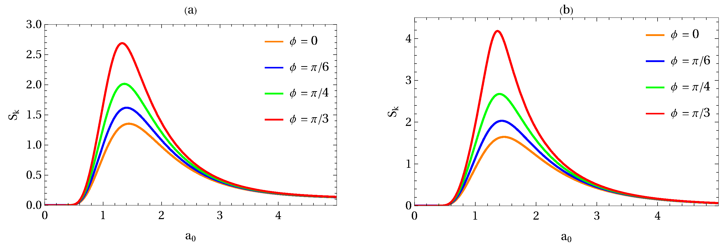
4. Particle Creation Entropy

For any arbitrary inertial observer, we can expand the solution of the motion equation as a sum of positive-frequency and negative-frequency solutions in asymptotic regions in the past (in-region) and in the future (out-region). Thus, we have two equivalent representations for the scalar field:

$$\begin{array}{cc}\hfill \varphi (x,\eta )& =\int d^{3}k[a_k^{\mathrm{in}}{u}_k^{\mathrm{in}}+a_k^{\mathrm{in}†}{u}_k^{\mathrm{in}\ast }]=\int d^{3}k[a_k^{\mathrm{out}}{u}_k^{\mathrm{out}}+a_k^{\mathrm{out}†}{u}_k^{\mathrm{out}\ast }],\hfill \end{array}$$

where the annihilation operators ($a_k^{\mathrm{in}\left(\mathrm{out}\right)}$) and creation operators ($a_k^{\mathrm{in}\left(\mathrm{out}\right)†}$) satisfy the usual commutation relation, i.e., $[a_k^{\mathrm{in}\left(\mathrm{out}\right)},a_{k^{\prime }}^{\mathrm{in}\left(\mathrm{out}\right)†}]={\delta }^3(k-k^{\prime })$ and $[a_k^{\mathrm{in}\left(\mathrm{out}\right)},a_{k^{\prime }}^{\mathrm{in}\left(\mathrm{out}\right)}]=[a_k^{\mathrm{in}\left(\mathrm{out}\right)†},a_{k^{\prime }}^{\mathrm{in}\left(\mathrm{out}\right)†}]=0$. By using the properties of the Klein–Gordon product, one can expand the ladder operators associated with one basis in terms of ladder operators of the other. For example, we have

$$\begin{array}{c}\hfill a_k^{\mathrm{out}}={\alpha }_k^{\ast }{a}_k^{\mathrm{in}}-{\beta }_k^{\ast }{a}_{-k}^{\mathrm{in}†}.\end{array}$$

(18)

where the ${\alpha }_k$ and ${\beta }_k$ coefficients are the Bogoliubov coefficients defined as ${\alpha }_k=(u_k^{\mathrm{out}},u_k^{\mathrm{in}})$ and ${\beta }_k=-(u_k^{\mathrm{out}},u_k^{\mathrm{in}\ast })$. As a consequence of the conformal symmetry of the theory, the computation of the Bogoliubov coefficients takes a diagonal form, and the Bogoliubov transformation only mix modes of the same k. Note also that the condition of $V\left(\eta \right)\to 0$ as $\eta \to \pm \infty$ will certainly be satisfied if spacetime is to be asymptotically flat in the distant past and the far future. More generally, it will be satisfied if one can define an adiabatic vacuum state in one of he two regions. This is the case in our present problem, where the in-region is an Einstein static state and the out-region is a de Sitter expansion phase. Thus, let us assume the initial vacuum state (in-vacuum) to be a Minkowski vacuum (${|0\rangle }_{\mathrm{in}}$) and the out-vacuum (${|0\rangle }_{\mathrm{out}}$) to be an adiabatic vacuum state (de Sitter-invariant vacuum). These vacuum states are defined as $a_k^{\mathrm{in}}{|0\rangle }_{\mathrm{in}}=0,$ and $a_k^{\mathrm{out}}{|0\rangle }_{\mathrm{out}}=0.$ If we now compute the expectation value of the number operator in the asymptotic future ($N_k^{\mathrm{out}}=a_k^{\mathrm{out}†}{a}_k^{\mathrm{out}}$) when the state of the field is the vacuum in the asymptotic past, we obtain

$$\begin{array}{c}\hfill {}_{\mathrm{in}}\langle 0\left|N_k^{\mathrm{out}}\right|0\rangle _{\mathrm{in}}={\left|{\beta }_k\right|}^2.\end{array}$$

(19)

By plugging the Equation (11) into Equation (19), we find that

$$\begin{array}{cc}\hfill {}_{\mathrm{in}}\langle 0\left|N_k^{\mathrm{out}}\right|0\rangle _{\mathrm{in}}& =|{\beta }_k^{\left(m\right)}+{\beta }_k^{\left(\xi \right)}+{\beta }_k^{\left(ϵ\right)}{|}^2,\hfill \\ \hfill & =|{\beta }_k^{\left(m\right)}{|}^2+|{\beta }_k^{\left(\xi \right)}{|}^2+{|{\beta }_k^{\left(ϵ\right)}|}^2+2\mathcal{R}\left[{\beta }_k^{\left(m\right)}{\beta }_k^{\left(\xi \right)}+{\beta }_k^{\left(m\right)}{\beta }_k^{\left(ϵ\right)}+{\beta }_k^{\left(\xi \right)}{\beta }_k^{\left(ϵ\right)}\right].\hfill \end{array}$$

(20)

This result implies that when ${\beta }_k^{\left(m\right)}$, ${\beta }_k^{\left(\xi \right)}$ and ${\beta }_k^{\left(ϵ\right)}$ are different from zero, one would observe particle production due to the dynamics of spacetime expansion. In addition, the relation between the different vacua is expressed by Schmidt decomposition as follows:

$$\begin{array}{c}\hfill |0_k{\rangle }_{\mathrm{in}}=\sum _{n=0}^{\infty }{c}_n^k|n_k{\rangle }_{\mathrm{out}}{|n_{-k}\rangle }_{\mathrm{out}},\end{array}$$

(21)

which means that the in-vacuum state can be seen as a two-mode squeezed state of modes k and $-k$ by an observer in the out-region. The Schmidt coefficients ($c_n^k$) encode Bogoliubov coefficients and can be evaluated as

$$\begin{array}{c}\hfill c_n^k=\sqrt{1-{\gamma }_k}{\left({\displaystyle \frac{{\beta }_k}{{\alpha }_k}}\right)}^n,\end{array}$$

where ${\gamma }_k={\left|{\displaystyle \frac{{\beta }_k}{{\alpha }_k}}\right|}^2.$ The amount of entanglement between particle and anti-particle modes in state (21) can be evaluated viathe von Neumann entropy of the reduced density matrix (${\widehat{\rho }}_k^{\mathrm{out}}$), i.e.,

$$\begin{array}{c}\hfill S_k=-\mathrm{Tr}\left[{\widehat{\rho }}_k^{\mathrm{out}}{log}_2{\widehat{\rho }}_k^{\mathrm{out}}\right],\end{array}$$

(22)

where

$$\begin{array}{cc}\hfill {\widehat{\rho }}_k^{\mathrm{out}}& ={\mathrm{Tr}}_{-k}\left[\right|0_k{0}_{-k}\rangle \mathrm{out}\langle 0_k{0}_{-k}\left|\right]=(1-{\gamma }_k)\sum _{n=0}^{\infty }{\gamma }_k^n|n_k{\rangle }_{\mathrm{in}}\langle n_k|.\hfill \end{array}$$

After some algebraic manipulations, one obtains

$$\begin{array}{c}\hfill S_k=-{log}_2(1-{\gamma }_k)-{\displaystyle \frac{{\gamma }_k}{1-{\gamma }_k}}{log}_2{\gamma }_k.\end{array}$$

(23)

5. Alice and Bob in an Expanding Spacetime

In this section, we consider a setup in which two comoving observers, Alice and Bob, possesses detectors sensitive to the same frequency mode of a massive scalar field. Initially, let us assume that in-region ($\eta \to -\infty$) Alice and Bob share the maximally entangled state, i.e.,

$$\begin{array}{c}\hfill |{\psi }_{AB}\rangle ={\displaystyle \frac{1}{\sqrt{2}}}\left[\right|0_{\mathrm{A}}\rangle |0_{\mathrm{B}}\rangle +|1_{\mathrm{A}}\rangle |1_{\mathrm{B}}\rangle ].\end{array}$$

(24)

Here, we suppose that the two detectors are assumed to be identical in all respects, except that they are spatially separated by a space-like interval. During the expansion phase of the Universe, Alice perceives Bob as receding from her in her local comoving frame. By using (21) and

$$\begin{array}{cc}\hfill |1_k{\rangle }_{\mathrm{in}}& =a_k^{\mathrm{in}†}{|0_k\rangle }_{\mathrm{in}},\hfill \\ \hfill & =({\alpha }_k{a}_k^{\mathrm{out}}-{\beta }_k{a}_{-k}^{\mathrm{out}†})\sum _{n=0}^{\infty }{c}_n^k|n_k{\rangle }_{\mathrm{out}}{|n_{-k}\rangle }_{\mathrm{out}},\hfill \\ \hfill & =(1-{\gamma }_k)\sum _{n=0}^{\infty }{c}_n^k\sqrt{n+1}|{(n+1)}_k{\rangle }_{\mathrm{out}}{|n_{-k}\rangle }_{\mathrm{out}},\hfill \end{array}$$

we can rewrite Equation (24) as

$$\begin{array}{c}\hfill |{\psi }_{AB}\rangle ={\displaystyle \frac{1}{\sqrt{2}}}\sum _{n=0}^{\infty }\left[c_n^k|0_{\mathrm{A}}\rangle |n_k{\rangle }_{\mathrm{out}}|n_{-k}{\rangle }_{\mathrm{out}}+d_n^k|1_{\mathrm{A}}{\rangle |(n+1)}_k{\rangle }_{\mathrm{out}}{|n_{-k}\rangle }_{\mathrm{out}}\right],\end{array}$$

(25)

where $d_n^k=(1-{\gamma }_k){\left({\displaystyle \frac{{\beta }_k}{{\alpha }_k}}\right)}^n\sqrt{n+1}$.

Quantum resources such as coherence and entanglement are known to encode information about the dynamical history of spacetime. By analyzing the quantum properties of the entangled state (25), specifically the $l_1$-norm coherence, it is possible to infer features of the underlying spacetime structure, including anisotropies in an emergent universe scenario. For simplicity, we assume that Bob’s detector is sensitive only to the particle mode (k). Under this assumption, the reduced density operator describing the bipartite system composed of Alice and Bob (mode k) is obtained by tracing over the antiparticle mode ($-k$):

$$\begin{array}{c}\hfill {\rho }_{A{B}_k}={\mathrm{Tr}}_{-k}\left[{\rho }_{AB}\right]={\displaystyle \frac{(1-{\gamma }_k)}{2}}\sum _{n=0}^{\infty }{\gamma }_k^n{\rho }_{A{B}_k}^n,\end{array}$$

where

$$\begin{array}{cc}\hfill {\rho }_{A{B}_k}^n& =|0_{\mathrm{A}},n_k\rangle \langle 0_{\mathrm{A}},n_k|+(1-{\gamma }_k)(n+1)|1_{\mathrm{A}},{(n+1)}_k\rangle \langle 1_{\mathrm{A}},{(n+1)}_k|\hfill \\ \hfill & +\sqrt{1-{\gamma }_k}\sqrt{n+1}|0_{\mathrm{A}},n_k\rangle \langle 1_{\mathrm{A}},{(n+1)}_k|+\sqrt{1-{\gamma }_k}\sqrt{n+1}|1_{\mathrm{A}},{(n+1)}_k\rangle \langle 0_{\mathrm{A}},n_k|.\hfill \end{array}$$

For simplicity, we omit the subscript “out” in the above expression. In the $\left\{\right|0_{\mathrm{A}},n_k\rangle ,|0_{\mathrm{A}},$${(n+1)}_k\rangle ,|1_{\mathrm{A}},n_k\rangle ,|1_{\mathrm{A}},{(n+1)}_k\rangle \}$ bases, we can write ${\rho }_{A{B}_k}^n$ in the matrix form as follows:

$$\begin{array}{c}\hfill {\rho }_{A{B}_k}^n=\left(\begin{array}{cccc}1& 0& 0& \sqrt{1-{\gamma }_k}\sqrt{n+1}\\ 0& 0& 0& 0\\ 0& 0& 0& 0\\ \sqrt{1-{\gamma }_k}\sqrt{n+1}& 0& 0& (1-{\gamma }_k)(n+1)\end{array}\right),\end{array}$$

In this paper, we are interested in quantifying the effects of cosmic expansion and the anisotropy of spacetime on the coherence and the quantum correlation of the final state shared between Alice and Bob. In general, the off-diagonal elements of a density matrix, when expressed in a chosen reference basis, characterize the coherence properties of a quantum state. In 2014, Baumgratz et al. [24] established a rigorous framework for quantifying coherence and identified computationally tractable measures for its evaluation. According to authors, for the quantum state described by density matrix $\rho$, the quantum coherence can be quantified in terms of the $l_1$-norm coherence (${\mathcal{C}}_{l_1}$), which is defined as ${\mathcal{C}}_{l_1}\left(\rho \right)={\sum }_{\mu \ne \nu }\left|{\rho }_{\mu \nu }\right|,$ where ${\mathcal{C}}_{l_1}\left(\rho \right)$ quantifies coherence as the sum of the absolute values of the off-diagonal elements of $\rho$. Therefore, the $l_1$-norm coherence of quantum state ${\rho }_{A{B}_k}$ is given by

$$\begin{array}{c}\hfill {\mathcal{C}}_{l_1}\left({\rho }_{A{B}_k}\right)={(1-{\gamma }_k)}^{{\displaystyle \frac{3}{2}}}\sum _{n=0}^{\infty }\sqrt{n+1}{\gamma }_k^n.\end{array}$$

(26)

Here, we are particularly interested in identifying the conditions under which the coherence of the final state becomes insensitive to variations in the expansion parameter, a phenomenon referred to as coherence freezing [30,49]. To investigate this regime, we analyze the derivative of the ${\ell }_1$-norm coherence ($C_{l_1}\left({\rho }_{A{B}_k}\right)$) with respect to a generic parameter ($\Gamma$, where $\Gamma \in \{a_0,H_0,m,k\}$). Specifically, coherence freezing occurs when this derivative vanishes, indicating that the measure of coherence remains unchanged under further increases in the $\Gamma$ parameter. Thus, the necessary condition for freezing can be obtained by evaluating

$${\displaystyle \frac{\partial C_{l_1}}{\partial \Gamma }}=0,\left(\mathrm{Freezing}\mathrm{Condition}\right).$$

In what follows, we compute this derivative explicitly and examine how the coherence dynamics depend on the acceleration scale, field mass, and anisotropy.

$$\begin{array}{c}\hfill {\displaystyle \frac{\partial C_{l_1}}{\partial \Gamma }}=\left\{-{\displaystyle \frac{3}{2}}{(1-{\gamma }_k)}^{{\displaystyle \frac{1}{2}}}\sum _{n=0}^{\infty }\sqrt{n+1}{\gamma }_k^n+{(1-{\gamma }_k)}^{{\displaystyle \frac{3}{2}}}\sum _{n=0}^{\infty }n\sqrt{n+1}{\gamma }_k^{n-1}\right\}{\displaystyle \frac{\partial {\gamma }_k}{\partial \Gamma }}.\end{array}$$

(27)

This equation vanishes only under two conditions: either ${\gamma }_k=1$, which corresponds to a trivial solution, or ${\displaystyle \frac{\partial {\gamma }_k}{\partial \Gamma }}=0$. The latter defines a nontrivial condition for the emergence of a frozen coherence regime. Consequently, such regimes can be identified through the numerical analysis of the ${\displaystyle \frac{\partial {\gamma }_k}{\partial \Gamma }}$ derivative. In the following section, we demonstrate that distinct freezing regimes arise depending on the specific values of the model parameters.

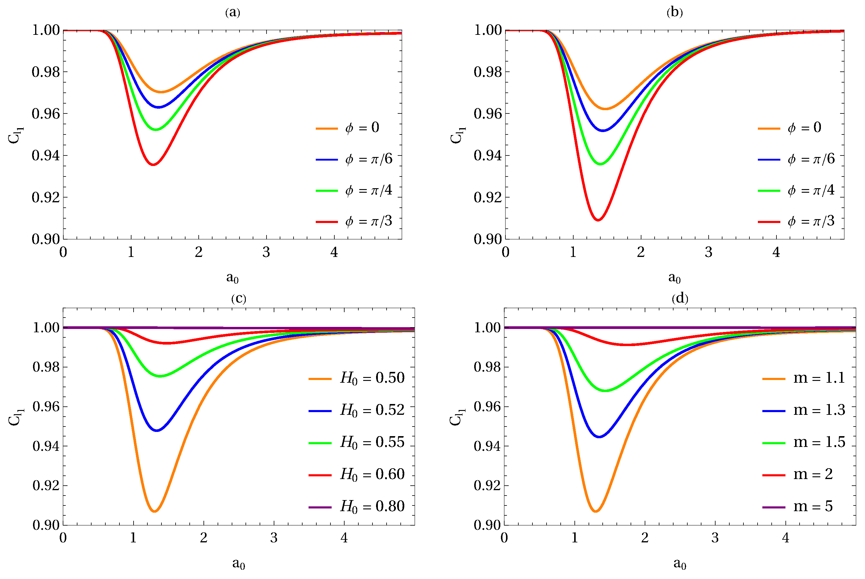
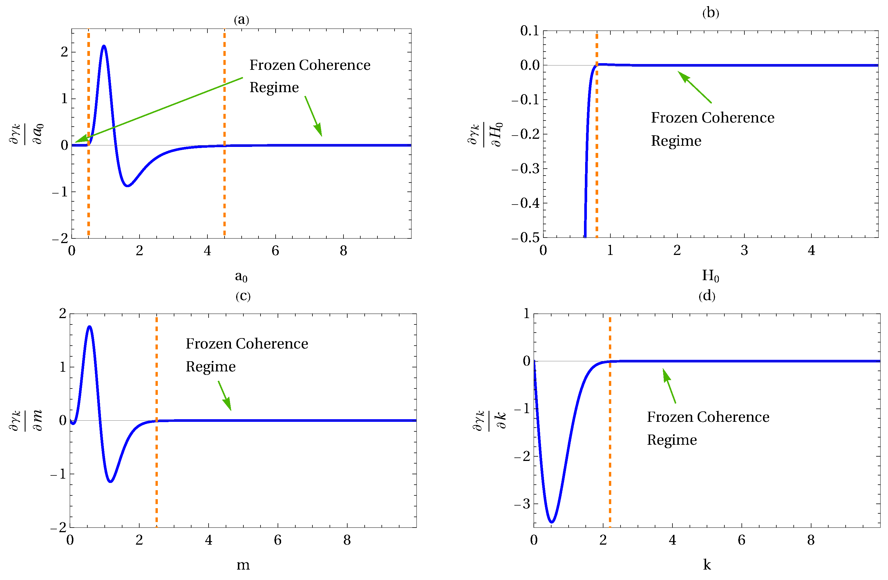
6. Numerical Results

In order to realize the numerical analysis, let us assume that wave vector $\overrightarrow{k}=(k_1,k_2,k_3)$ has a general direction specified by spherical coordinates $(k,\theta ,\varphi )$ as $\overrightarrow{k}=k_{x}sin\theta cos\varphi {\widehat{e}}_x+k_{y}sin\theta sin\varphi {\widehat{e}}_y+k_{z}cos\theta {\widehat{e}}_z,$ where $k^2=k_x^2+k_y^2+k_z^2$. Notice that the effects of the anisotropy are expected to depend upon the direction of the particle momentum. Thus, the influence of anisotropy on the entanglement entropy, coherence, and quantum correlation can be quantified by the azimuthal angle ($\varphi$) and the polar angle ($\theta$).

Figure 2 shows particle creation entropy as a function of the $a_0$ parameter for different values of the azimuthal angle ($\varphi$). Notice that entanglement entropy exhibits non-monotonic spectral behavior, i.e., entanglement entropy initially increases to a maximum value, then decreases to a fixed value. This suggest that spacetime’s dynamics of an emergent universe can produce non-local quantum correlation. In addition, there is an optimal value of $a_0$ that favors the encoding of information about the effects of spacetime’s dynamics of an emergent universe. Another thing to note is that the behavior of entanglement entropy is very similar for minimal ($\xi =0$) and conformal ($\xi =1/6$) coupling.

In Figure 3, we plot the coherence equation (Equation (26)) as a function of the expansion parameter ($a_0$). The results show that the coherence initially decreases to a minimum value and subsequently increases, approaching unity as $a_0$ increases.

Figure 3a,b illustrate that the minimum value of coherence increases as the $\varphi$ parameter varies from 0 to $\pi /3$, indicating the influence of anisotropy on the coherence of the final state shared between Alice and Bob. Regarding the effect of the coupling parameter ($\xi$) on coherence, the behavior remains qualitatively similar for minimal coupling ($\xi =0$) and conformal coupling ($\xi =1/6$), as shown in the same figures. In contrast, Figure 3c,d reveal that the minimum coherence gradually diminishes as either $H_0$ or m increases. Notably, coherence remains unchanged for sufficiently large values of $H_0$ or m, suggesting the emergence of a frozen coherence regime when $H_0\gtrsim 0.80$ or $m\gtrsim 2.5$.

Figure 4 shows the behavior of ${\displaystyle \frac{\partial {\gamma }_k}{\partial \Gamma }}$ with respect to the set parameters of $\{a_0,H_0,m,k\}$. This numerical analysis of ${\displaystyle \frac{\partial {\gamma }_k}{\partial \Gamma }}$ provides the dynamical conditions that lead to coherence freezing. From Figure 4a, we can see that ${\displaystyle \frac{\partial {\gamma }_k}{\partial a_0}}$ exhibits oscillatory behavior for values of $a_0$ between $0.5$ and $4.5$. In addition, notice that there are two frozen coherence regimes when $a_0\lesssim 0.5$ and $a_0\gtrsim 4.5$. This suggests that coherence freezing can occur in both early (quasi-static) and late (quasi-de Sitter) phases of an emergent universe. Figure 4b shows that when $H_0\gtrsim 0.80$, ${\displaystyle \frac{\partial {\gamma }_k}{\partial H_0}}\to 0$, implying that rapid expansion suppresses curvature-induced mode mixing. Similarly, Figure 4c,d show that coherence freezing occurs for field masses of $m\gtrsim 2.5$ and momenta of $k\gtrsim 2.2$, highlighting the significance of high-energy modes in the stabilization of quantum coherence.

The results depicted in Figure 4 demonstrate that coherence freezing occurs when the values of the $\{a_0,H_0,m,k\}$ parameters lie within the specific regimes outlined in

Table 1. Frozen coherence regimes.

	Parameter
Spacetime	$0.5\gtrsim a_0\gtrsim 4.5$
Spacetime	$H_0\gtrsim 0.80$
Field	$m\gtrsim 2.5$
Field	$k\gtrsim 2.2$

. Within these regimes, the $l_1$-norm coherence becomes effectively insensitive to variations in the expansion parameters, suggesting that the quantum features of the bipartite state shared by comoving observers remain preserved throughout the cosmic evolution of the emergent Universe. The origin of this robustness of coherence can be attributed to the suppression of particle creation ($|{\beta }_k|\to 0$). This corroborates the fact that the weak curvature of spacetime or high-frequency modes minimizes the impact of curvature-induced mode mixing, thereby protecting quantum resources.

In contrast to isotropic models, such as those investigated in Refs. [35,39,40], our findings suggest that the presence of anisotropy introduces a directional dependence in the evolution of quantum features. In particular, coherence exhibits sensitivity to the azimuthal angle ($\varphi$), which serves as a direct probe of the spacetime anisotropy. In addition, the freezing regimes identified in this work are obtained within the approximation of a purely classical background spacetime. In such regimes, the quantum scalar field does not significantly alter the geometry (i.e., backreaction is neglected). Our findings offer a preliminary characterization of the behavior of quantum coherence in an anisotropic expanding spacetime. It is important to emphasize that the results presented here are model-dependent. Nevertheless, the observed qualitative features, such as the directional dependence of quantum coherence and the emergence of freezing regimes, are expected to be generic properties of non-singular cosmological models exhibiting asymptotic behavior with small anisotropic perturbations.

7. Concluding Remarks

In summary, we have investigated the dynamics of quantum coherence in an anisotropic emergent universe. In particular, we studied how cosmic expansion, frequency modes, and small anisotropic perturbations affect quantum coherence encoding in the modes of a massive scalar field. First, our numerical analyses show that the presence of anisotropy introduces a directional dependence in the dynamics of quantum features, i.e., the quantum coherence exhibits sensitivity to the azimuthal angle ($\varphi$), which serves as a direct probe of the spacetime anisotropy. Secondly, we found the emergence of frozen coherence regimes when the $\{a_0,H_0,m,k\}$ parameters lie within particular ranges, as summarized in Table 1. The origin of these frozen regimes can be attributed to the suppression of Bogoliubov mode mixing and, consequently, to reduced particle creation ($|{\beta }_k|\to 0$).

Additionally, the analysis of ${\displaystyle \frac{\partial {\gamma }_k}{\partial \Gamma }}=0$, where $\Gamma \in \{a_0,H_0,m,k\}$ (Figure 4) shows that high-frequency modes and large expansion rates contribute significantly to the stability of coherence. These findings support the physical interpretation according to which quantum features can remain robust during the early expansion phases of the Universe, provided that the spacetime curvature and anisotropy are not strong enough to induce significant particle creation. According to our findings, the identification of coherence freezing regimes in expanding spacetimes offers promising avenues for the exploration of the persistence of quantum properties in the early Universe and their potential relevance to quantum information theory in relativistic contexts. This approach can be extended to other types of quantum fields, non-Gaussian initial states, and more general cosmological backgrounds such as bouncing and cyclic models. These directions are left for future investigation.

References

1. Nielsen, M.A.; Chuang, I.L. Quantum Computation and Quantum Information, 10th ed.; Cambridge University Press: Cambridge, UK, 2010. [Google Scholar]
2. Streltsov, A.; Adesso, G.; Plenio, M.B. Quantum coherence as a resource. Rev. Mod. Phys. 2017, 89, 041003. [Google Scholar] [CrossRef]
3. Hillery, M. Coherence as a resource in decision problems: The Deutsch-Jozsa algorithm and a variation. Phys. Rev. A 2016, 93, 012111. [Google Scholar] [CrossRef]
4. Pan, M.; Qiu, D. Operator coherence dynamics in Grover’s quantum search algorithm. Phys. Rev. A 2019, 100, 012349. [Google Scholar] [CrossRef]
5. Ahnefeld, F.; Theurer, T.; Egloff, D.; Matera, J.M.; Plenio, M.B. Coherence as a Resource for Shor’s Algorithm. Phys. Rev. Lett. 2022, 129, 120501. [Google Scholar] [CrossRef]
6. Karimi, M.; Javadi-Abhari, A.; Simon, C.; Ghobadi, R. The power of one clean qubit in supervised machine learning. Sci. Rep. 2023, 13, 19975. [Google Scholar] [CrossRef]
7. Giovannetti, V.; Lloyd, S.; Maccone, L. Quantum-Enhanced Measurements: Beating the Standard Quantum Limit. Science 2004, 306, 1330–1336. [Google Scholar] [CrossRef]
8. Giovannetti, V.; Lloyd, S.; Maccone, L. Advances in quantum metrology. Nat. Photonics 2011, 5, 222–229. [Google Scholar] [CrossRef]
9. Demkowicz-Dobrzański, R.; Maccone, L. Using Entanglement Against Noise in Quantum Metrology. Phys. Rev. Lett. 2014, 113, 250801. [Google Scholar] [CrossRef]
10. Aberg, J. Catalytic Coherence. Phys. Rev. Lett. 2014, 113, 150402. [Google Scholar] [CrossRef]
11. Narasimhachar, V.; Gour, G. Low-temperature thermodynamics with quantum coherence. Nat. Commun. 2015, 6, 7689. [Google Scholar] [CrossRef]
12. Ćwikliński, P.; Studziński, M.; Horodecki, M.; Oppenheim, J. Limitations on the Evolution of Quantum Coherences: Towards Fully Quantum Second Laws of Thermodynamics. Phys. Rev. Lett. 2015, 115, 210403. [Google Scholar] [CrossRef]
13. Lostaglio, M.; Jennings, D.; Rudolph, T. Description of quantum coherence in thermodynamic processes requires constraints beyond free energy. Nat. Commun. 2015, 6, 6383. [Google Scholar] [CrossRef]
14. Plenio, M.B.; Huelga, S.F. Dephasing-assisted transport: Quantum networks and biomolecules. New J. Phys. 2008, 10, 113019. [Google Scholar] [CrossRef]
15. Huelga, S.F.; Plenio, M.B. Vibrations, quanta and biology. Contemp. Phys. 2013, 54, 181–207. [Google Scholar] [CrossRef]
16. Li, C.-M.; Lambert, N.; Chen, Y.-N.; Chen, G.-Y.; Nori, F. Witnessing Quantum Coherence: From solid-state to biological systems. Sci. Rep. 2012, 2, 885. [Google Scholar] [CrossRef]
17. Levi, F.; Mintert, F. A quantitative theory of coherent delocalization. New J. Phys. 2014, 16, 033007. [Google Scholar] [CrossRef]
18. Karpat, G.; Cakmak, B.; Fanchini, F.F. Quantum coherence and uncertainty in the anisotropic XY chain. Phys. Rev. B 2014, 90, 104431. [Google Scholar] [CrossRef]
19. Girolami, D. Observable Measure of Quantum Coherence in Finite Dimensional Systems. Phys. Rev. Lett. 2014, 113, 170401. [Google Scholar] [CrossRef]
20. Cakmak, B.; Karpat, G.; Fanchini, F. Factorization and Criticality in the Anisotropic XY Chain via Correlations. Entropy 2015, 17, 790–817. [Google Scholar] [CrossRef]
21. Malvezzi, A.L.; Karpat, G.; Cakmak, B.; Fanchini, F.F.; Debarba, T.; Vianna, R.O. Quantum correlations and coherence in spin-1 Heisenberg chains. Phys. Rev. B 2016, 93, 184428. [Google Scholar] [CrossRef]
22. Chen, J.J.; Cui, J.; Zhang, Y.R.; Fan, H. Coherence susceptibility as a probe of quantum phase transitions. Phys. Rev. A 2016, 94, 022112. [Google Scholar] [CrossRef]
23. Li, Y.; Lin, H. Quantum coherence and quantum phase transitions. Sci. Rep. 2016, 6, 26365. [Google Scholar] [CrossRef]
24. Baumgratz, T.; Cramer, M.; Plenio, M. Quantifying coherence. Phys. Rev. Lett. 2014, 113, 140401. [Google Scholar] [CrossRef]
25. Shao, L.-H.; Xi, Z.; Fan, H.; Li, Y. Fidelity and trace-norm distances for quantifying coherence. Phys. Rev. A 2015, 91, 042120. [Google Scholar] [CrossRef]
26. Rastegin, A.E. Quantum-coherence quantifiers based on the Tsallis relative α entropies. Phys. Rev. A 2016, 93, 032136. [Google Scholar] [CrossRef]
27. Chitambar, E.; Gour, G. Comparison of incoherent operations and measures of coherence. Phys. Rev. A 2016, 94, 052336. [Google Scholar] [CrossRef]
28. Wang, S.-C.; Yu, Z.-W.; Zhou, W.-J.; Wang, X.-B. Protecting quantum states from decoherence of finite temperature using weak measurement. Phys. Rev. A 2014, 89, 022318. [Google Scholar] [CrossRef]
29. Wang, Y.-K.; Fei, S.-M.; Wang, Z.-X. Dynamics of quantum coherence in Bell-diagonal states under Markovian channels. Commun. Theor. Phys. 2019, 71, 555. [Google Scholar] [CrossRef]
30. Bromley, T.R.; Cianciaruso, M.; Adesso, G. Frozen Quantum Coherence. Phys. Rev. Lett. 2015, 114, 210401. [Google Scholar] [CrossRef]
31. Yu, X.-D.; Zhang, D.-J.; Liu, C.L.; Tong, D.M. Measure-independent freezing of quantum coherence. Phys. Rev. A 2016, 93, 060303. [Google Scholar] [CrossRef]
32. Silva, I.A.; Souza, A.M.; Bromley, T.R.; Cianciaruso, M.; Marx, R.; Sarthour, R.S.; Oliveira, I.S.; Franco, R.L.; Glaser, S.J.; deAzevedo, E.R.; et al. Observation of Time-Invariant Coherence in a Nuclear Magnetic Resonance Quantum Simulator. Phys. Rev. Lett. 2016, 117, 160402. [Google Scholar] [CrossRef]
33. Yu, S.; Wang, Y.-T.; Ke, Z.-J.; Liu, W.; Zhang, W.-H.; Chen, G.; Tang, J.-S.; Li, C.-F.; Guo, G.-C. Experimental realization of self-guided quantum coherence freezing. Phys. Rev. A 2017, 96, 062324. [Google Scholar] [CrossRef]
34. Shi, J.; Chen, J.; He, J.; Wu, T.; Ye, L. Inevitable degradation and inconsistency of quantum coherence in a curved space-time. Quantum Inf. Process. 2019, 18, 300. [Google Scholar] [CrossRef]
35. Huang, Z.; Situ, H. Quantum coherence behaviors of fermionic system in non-inertial frame. Quantum Inf. Process. 2018, 17, 95. [Google Scholar] [CrossRef]
36. Huang, Z. Dynamics of quantum correlation and coherence in de Sitter universe. Quantum Inf. Process. 2017, 16, 207. [Google Scholar] [CrossRef]
37. Wu, S.-M.; Wang, C.-X.; Wang, R.-D.; Li, J.-X.; Huang, X.-L.; Zeng, H.-S. Curvature-enhanced multipartite coherence in the multiverse. Chin. Phys. C 2024, 48, 075107. [Google Scholar] [CrossRef]
38. Du, M.-M.; Li, H.-W.; Tao, Z.; Shen, S.-T.; Yan, X.-J.; Li, X.-Y.; Zhong, W.; Sheng, Y.-B. Basis-independent quantum coherence and its distribution under relativistic motion. Eur. Phys. J. C 2024, 84, 838. [Google Scholar] [CrossRef]
39. Wu, S.-M.; Wang, C.-X.; Liu, D.-D.; Huang, X.-L. Would quantum coherence be increased by curvature effect in de Sitter space? J. High Energy Phys. 2023, 2023, 115. [Google Scholar] [CrossRef]
40. Wu, S.-M.; Zeng, H.-S.; Liu, T. Quantum correlation between a qubit and a relativistic boson in an expanding spacetime. Class. Quantum Gravity 2022, 39, 135016. [Google Scholar] [CrossRef]
41. Parker, L. Quantized fields and particle creation in expanding universes. Part 1. Phys. Rev. 1969, 183, 1057. [Google Scholar] [CrossRef]
42. Parker, L. Quantized fields and particle creation in expanding universes. Part 2. Phys. Rev. D 1971, 3, 346. [Google Scholar] [CrossRef]
43. Birrell, N.D.; Davies, P.C.W. Quantum Fields in Curved Space; Cambridge University Press: Cambridge, UK, 1982. [Google Scholar]
44. Ford, L.H. Cosmological particle production: A review. Rep. Prog. Phys. 2021, 84, 116901. [Google Scholar] [CrossRef]
45. Zeldovich, Y.A. Particle Creation and Vacuum Polarization in Anisotropic Gravitational Field. Zh. Exp. Theor. Fiz. 1971, 61, 2161–2175. [Google Scholar]
46. Birrell, N.D. Momentum space techniques for curved space–time quantum field theory. Proc. R. Soc. Lond. A 1979, 367, 123–141. [Google Scholar]
47. Ellis, G.F.R.; Murugan, J.; Tsagas, C.G. The emergent universe: An explicit construction. Class. Quantum Gravity 2003, 21, 233. [Google Scholar] [CrossRef]
48. Ellis, G.F.R.; Maartens, R. The emergent universe: Inflationary cosmology with no singularity. Class. Quantum Gravity 2003, 21, 223. [Google Scholar] [CrossRef]
49. Bai, Z.; Du, S. Frozen condition of quantum coherence. Phys. Scr. 2024, 99, 105102. [Google Scholar] [CrossRef]
Figure 1. Illustration of an emergent universe. The Universe originates from an Einstein static state, then evolves into an inflationary epoch. η t represents the transition time.
Universe 11 00185 g001
Figure 2. Entanglement entropy as a function of the a 0 parameter for different values of the azimuthal angle ( ϕ ). (a) ξ = 0 ; (b) ξ = 1 / 6 . Here, we fixed k = 1 , m = 1.1 , H 0 = 0.5 , and θ = π / 2 .
Universe 11 00185 g002
Figure 3. Coherence as a function of the a 0 parameter for different values of the azimuthal angle ( ϕ ). (a) ξ = 0 ; (b) ξ = 1 / 6 . Here, we fixed k = 1 , m = 1.1 , H 0 = 0.5 , and θ = π / 2 . (c) Coherence as a function of the a 0 parameter for different values of the H 0 parameter. Here, we fixed k = 1 , m = 1.1 , ξ = 0 , and θ = ϕ = π / 2 . (d) Coherence as a function of the a 0 parameter for different values of m. Here, we fixed k = 1 , H 0 = 0.5 , ξ = 0 , and θ = ϕ = π / 2 .
Universe 11 00185 g003
Figure 4. (a) γ k a 0 as a function of the a 0 parameter. Here, we fixed ξ = 0 , k = 1 , m = 1.1 , H 0 = 0.5 , and θ = ϕ = π / 2 . (b) γ k H 0 as a function of the H 0 parameter. Here, we fixed ξ = 0 , k = 1 , m = 1.1 , a 0 = 1 , and θ = ϕ = π / 2 . (c) γ k m as a function of the mass (m). Here, we fixed ξ = 0 , k = 1 , a 0 = 1 , H 0 = 0.5 , and θ = ϕ = π / 2 . (d) γ k k as a function of the k parameter. Here, we fixed ξ = 0 , m = 1.1 , a 0 = 1 , H 0 = 0.5 , and θ = ϕ = π / 2 .
Universe 11 00185 g004