Abstract
With the great Clementine Gnomon in St. Maria degli Angeli, a 45 m pinhole meridian line, built in 1700–1702 upon the will of Pope Clemens XI, Francesco Bianchini inaugurated the Roman tradition of solar astrometry. We analyze two thousand dedicated observations at the Clementine Gnomon between 2018 and 2025, with solar altitudes from 20° to 71° and in various meteorological conditions, in order to assess the observational uncertainties on the solar diameter and their causes. We compare the meridian diameters measured by Bianchini near the winter solstices of 1701–1702 with the ones measured by Sigismondi in 2018–2025, reporting the observational errorbars per single measure and the systematic diminutions of the observed diameters with respect to the ephemerides, due to the turbulence and image contrast loss. Simulated datasets based on our measured uncertainties show that pinhole meridian lines cannot resolve solar diameter variations smaller than 1″ over 80 years. These limitations prevent tighter constraints on solar evolution across centuries using such instruments.
1. Structure of the Article
The Clementine Gnomon and the historical background of the pinhole meridian lines in the churches used as observatories in 17th and 18th centuries are presented in Section 2. In Section 3, we introduce the study on the solar parameters during the Maunder minimum. In Section 4, we present the observations at the Clementine Gnomon in Rome, used for the modern observations of the Sun (2018–2025). The local turbulent seeing affects the measures of the meridian lengths of the solar image. Geometrical and environmental factors, the meteorology, and the reflecting conditions of the marbles on and out of the meridian line are examined to understand the uncertainties of the observations. The measures of Bianchini in the winter solstices of 1701–1702 are presented in Section 5, and they are compared with the measure of Sigismondi (2018–2025) in Section 6. In Section 7, we approach the problem of the secular variation in the solar diameter and its detectability, through simulations with realistic errorbars obtained from the observations.
Finally, in Section 8, we discuss how our data contribute to unveiling the observational uncertainties in the 17th and 18th century.
2. The Clementine Gnomon and Its Historical Background
The Clementine Gnomon, also called the Meridian Line of St. Maria degli Angeli in Rome, is the instrument that we used to compare XVIII century observations to the present ones. It was built between 1700 and 1702 under the direction of the astronomer Mons. Francesco Bianchini (1662–1729). The Gnomon was financed by the Cardinal Gian-Francesco Albani before becoming Pope on 23 November 1700, with the name of Clemens XI (1700–1721).
This instrument is a gigantic pinhole camera designed to obtain an unprecedented accuracy in the daily meridian positions of the Sun, in order to measure the length of the tropical year, and the secular variations in the obliquity of the ecliptic. A horizontal pinhole of 25 mm diameter illuminates the meridian line nowadays.
Bianchini studied in Bologna and in Padova. He came into contact with the most prominent scholars of his time [1,2]. With the Clementine Gnomon, Bianchini designed the most advanced instrument of his time to assess the bases of the Gregorian Reformation of the Calendar in 1582. Newton invited Bianchini to join the Royal Society of London as a foreign fellow. The Clementine Gnomon remained, after Bianchini, a reference instrument also studied by Celsius in 1734 and Boscovich in 1750 [1].
Bianchini (1703) improved the instrumental performances of the Gnomon, with respect to the Heliometer of Bologna, using better-reflecting marbles, enabling observations of brighter stars from the meridian line, to obtain the sidereal time through their meridian transits, and making a very stable pinhole carved in the Diocletian’s walls, 1400 years old [1]. For each observation, Bianchini [3,4] darkened the Basilica with fabric applied to the windows from outside, and the observations started some hours before the meridian transit, a time necessary for total obscuration of the Basilica.
In 1750, the cotto tiles of the floor of the Basilica were renovated by Luigi Vanvitelli with marbles. The whole meridian line and the starred paths of the stars Sirius and Arcturus and the paths of the Sun on the equinoxes and on 20 August 1702 (visit of Clemens XI) spread on the floor of the Basilica were preserved.
The function of civil time keeping of the Clementine Gnomon ceased in 1846, when the Collegio Romano Observatory took this service: a big ball left falling along a tube, on top of St. Ignatius’ Church, was the visual signal for shooting the cannon on Castel St. Angelo [5,6].
Historical Context: Churches as Observatories
The previous instruments dedicated to measure the Earth’s orbit and obliquity are in the Cathedral of Florence designed by Toscanelli in 1475 (the gnomon of the Cathedral of Santa Maria del Fiore) and in Bologna in the Basilica of St. Petronio. Egnazio Danti made the first version in 1577 [7]; Cassini completely re-traced it in 1655 and restaured it in 1695 [8].
Giovan Domenico Cassini (1625–1712) and his collaborators monitored the solar diameter from 1655. Eustachio Manfredi [9] reported their and his observations, already corrected for the “penumbra” (the pinhole size) and for refraction effects. Tovar et al. [10] analyzed these data, concluding that the data of 1655–1715 in the grand sunspots’ minimum, and the ones of 1716–1736 immediately after, are compatible with the same solar diameter, within 0.6″.
With the meridian line created by De Cesaris in 1782 in the Duomo of Milan, the accuracy of the meridian’s azimuth reached 6″, but the astrometric purposes were no more in the scopes of its construction [11]. The meridian in the Cathedral of Palermo created by Piazzi in 1803 was devoted to the local noon’s determination for the Angelus’ prayer and for public timing, without any more astrometric scopes. The local noon gradually ceased to be relevant for public life, beyond religion, as World time zones and their mean time become in official use after the conference of Washington of 1884.
3. Secular Variations in the Solar Parameters in the Maunder Minimum
Since the antiquity, the Sun was considered as a celestial spherical body of fixed radius and given orbital motion. The variation in the distance with the Earth would change its angular diameter, according to the form and the center of its orbit. Cassini realized the meridian line of Bologna in 1655 to measure the solar angular diameter along the year and the irregularity of the Earth’s orbit.
The number of sunspots was the first solar parameter to be identified as variable, since the first observations of Galileo [12], and H. Schwabe [13] found a 10-year regularity, decades after him this was recognized as a 11-year cycle. E. W. Maunder and his wife [14,15] discovered, in archive data, a long period almost completely without spots, which nowadays is called the Maunder minimum. Finally, other great solar minima [16] were discovered and J. Eddy proposed to dedicate these periods to Oort (period around 1040) and to Spörer (in 15th century) [17].
Carrasco and Vaquero [18] studied the Sun’s rotation during the Maunder minimum from the correspondence of John Flamsteed. The aspect of the sunspots at the beginning of the minimum as observed by Hevelius was analyzed by Carrasco, Vaquero, Gallego et al., [19] as well as the umbra/penumbra ratio during the Maunder minimum (Carrasco, Garcia-Romero, Vaquero et al. [20]) and observations with the naked eye in the same period (Carrasco, Gallego, Arlt et al. [21]).
Several authors (e.g., [22,23]); Penza et al. [24] studied the variations in the solar irradiance correlated with the little ice age, which occurred in 17th and 18th centuries.
4. Modern Solar Observations at the Clementine Gnomon
Since 1999 C., Sigismondi has measured the positions of the Sun with respect to some fixed points (solstices, equinoxes, and some centesimal parts on the line. The nutation and the obliquity variations are measurable all days of the year (Sullivan, [25]), with a particularly high accuracy around the winter solstice, with a 1.77″/mm scaling at the meridian transit. The pinhole was found not to be calibrated with the rest of the meridian line, because of un-documented changes in its shape and position. In 2018, the pinhole was re-shaped and calibrated. On 27 October 2018, Costantino Sigismondi started an extensive astrometric observational campaign called IGEA (Informatized Geometric Ephemerides for Astrometry) with ZIA (Zenithal Imaging Analysis) in order to obtain accurate local references along the meridian line [26].
- The meridian measures of the solar diameter have been accompanied by meteorological data (pressure, temperature, and humidity) and sky aspects (cloudy, with veils or clear) to understand their contributions to the observed diameter’s length.
- All the meridian transits have been recorded and they are available on YouTube. (https://www.youtube.com/channel/UCe18v3EZ8w2qmd8jW6mYV5w/videos accessed on 4 June 2025 search “Transito meridiano a S. Maria degli Angeli” + the date in Italian, e.g., “3 maggio 2025”).
- The daily meridian positions of the solar limbs on the brass line are compared with the ephemerides to disentangle systematics from the astronomical seeing, meteorological, and personal equations.
Several sunspots during the present XXV solar cycle were visible on the meridian marbles, especially in the winter’s season, when the solar image was as large as hundred times the effective pinhole’s size: the highest resolution for such lensless telescope [27] is reached.
With a routine written in Excel, we compare the observed data with the predicted ones by the ephemerides. In the text we will consider the differences between our measures and the ephemerides (Stellarium 0.20 for present times or NASA for 18th century [28]) as O-C “observed minus calculated” data.
The solar diameter measured by Cassini, Bianchini, and by us is the length between the two meridian limbs of North and South; it is shorter than the ephemerides because of the following:
- a.
- The signal to noise ratio reduced by meteorological conditions and ambient light;
- b.
- Solar limb darkening;
- c.
- The penumbra (diameter of the horizontal pinhole, fixed);
- d.
- The cylinder effect (pinhole vertical thickness, which changes the effective pinhole area);
- e.
- The light reflected inside the marble, which enlarges the image southwards in summer time;
- f.
- The airmass extinction combined with the effective pinhole area.
The meridian diameter is then systematically 9 mm less than the ephemerides near the winter solstices (2018–2024), and it becomes 4 mm less at the half-meridian line and about 2 mm less in summer time. The intensity of the summer image is 5 times larger than in winter. Moreover a meteorological fluctuation of ±1.5 mm may appear as the meteo departs from STP (15 °C, 1013 hPa): at approximately 1 mm/10 °C and 1 mm/10 hPa near the winter solstice, the effect is less evident at lower focal lengths (distance pinhole image), i.e., toward summer time.
Nevertheless, near the meridian line, the motion of the image is perpendicular to the meridian line and this allows one to very precisely detect the limbs, if a fit over five positions per limb (pencil’s signs) is performed, and the center of the image can be located with a nominal precision often better than 1 mm.
4.1. The Pinhole of the Clementine Gnomon
The present pinhole is a cylinder 6.2 mm thick and 25 mm wide; this reduces the effective pinhole to about 11 mm meridian per 23 mm transverse in winter time, moving its center up to 7 mm in the meridian direction, periodically, during the year.
Originally, in 1702, the pinhole was a horizontal circle 20 mm wide, 1:1000 of its height [29]; it was designed by Giuseppe Campani (1635–1715), the best lens maker of his times, on a 2 mm-thick bronze plate [30].
The solar limb darkening convolutes with the pinhole aperture (called penumbra, because from there a part of the sky around the Sun is visible through the pinhole) and the diffraction produces a red rim of the solar image, up to 5 mm or 10″ width at the winter solstice. A dimmer ring of penumbra is always visible, especially in video.
4.2. The Meridian Line and Its Marbles
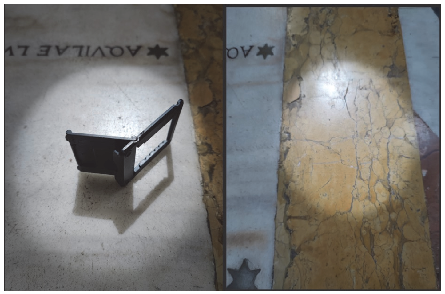
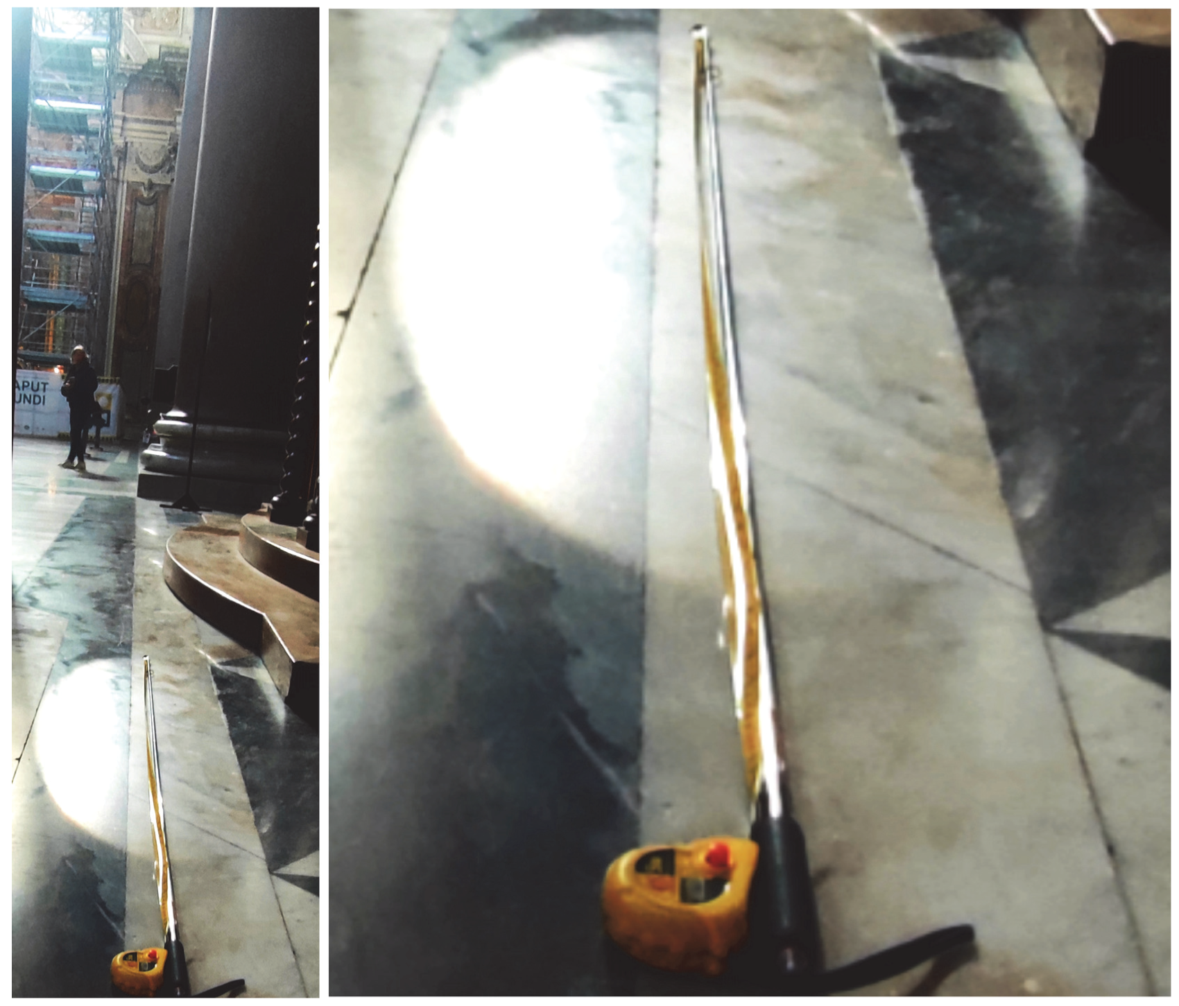
The central brass meridian line is 30 mm wide. It is inserted in two white marble slabs (910 mm width in total) and in two external yellow marble strips of 224 mm each (see Figure 1). The whole design is symmetrical, to enable the possibility to measure the meridian positions of the Sun ± 7.5 min from the meridian transit.

Figure 1.
The Sun with veiled sky on 9 April 2025. The light passing below the dark obstacle (left) is reflected inside the white marble; the image is on the yellow marble of Verona (right). The veiled sky showed a 22° halo around the Sun that day.
The reflection inside the marble is non-symmetrical because it is sensitive to the direction of the light, and on the Northern limb, closer to the pinhole (upper part of Figure 1), the light spreads into the solar image, while in the Southern limb, it spreads out, enlarging the measured diameter.
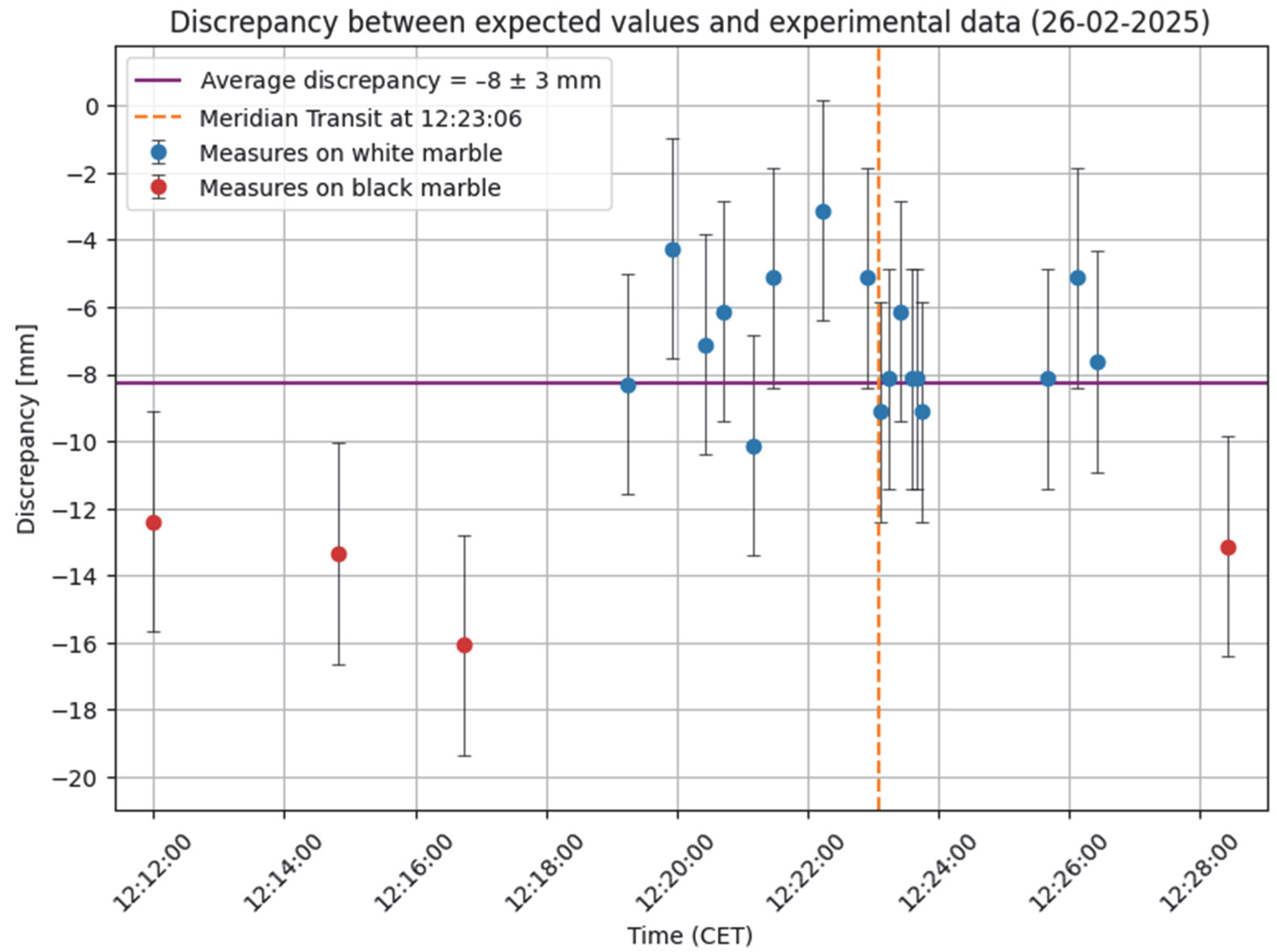
Moreover, the reflection on different marbles changes the perceived diameter (Figure 2 and Figure 3).

Figure 2.
Measured diameters (observed–calculated) in different meteorological conditions and on differently reflecting marbles in St. Maria degli Angeli (26 February 2025, video). The brown line indicates the time of the meridian transit (12:23:06 Central European Time, on that day). The blue dots with their dispersions are the measured meridian diameters on different marbles.

Figure 3.
The red-ringed image of the Sun at 9:43:22 of 11 February 2025. Its length is 1260 mm. A movable screen was necessary to see the image on the floor with such high ambient light and such low contrast.
4.3. Extra-Meridian Measurements on Vanvitelli’s Marbles
The pinhole casts the solar image on the marbles of the floor of the Basilica about 2 h before the meridian transits and its length can be measured, similarly to the meridian cases, marking the limbs of the major axis with a pencil on the polished marbles of Vanvitelli on the floor.
These marks are not simultaneous for both limbs, and the motion of the image off-meridian immediately covers the limb closer to the pinhole (the Sun is rising).
We could evaluate the lengths of the images and their statistical dispersions in different seasons, airmasses, and with different weathers.
We assume them to be similar to the one experienced by Bianchini in Rome and by Cassini and collaborators in Bologna.
The extra-meridian measurements taken in 2024–2025 aim to verify the observing conditions with solar altitudes ranging from 20° to 67°, the same range of the meridian transits in Bologna. With tens of measures in a single observing session, instead of a single meridian transit per day, we strengthen the statistics of our measurements. Over one thousand such observations (Figure 4) have been collected, along with meteorological data of pressure, temperature, and humidity and the opacity/clearness of the solar image.
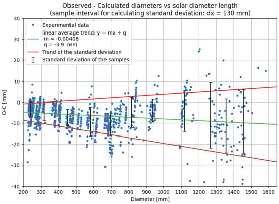
Figure 4.
Extra-meridian measures (1248 points) from December 2024 to June 2025 at the Clementine Gnomon. The differences between the observed and the measured diameters are plotted vs. the diameters of the images. The standard deviations of the measures increase linearly with the diameter. The diameters (major axis) are binned each dx = 130 mm, ranging from 225 mm to 1600 mm. The fitting green line has parameters y = mx + q plotted in the figure. The green line represents the systematic reduction in the measured diameter with respect to the ephemerides: the angular reduction ranges around −18″ all year. The standard deviations of the daily measures also change with the season and they are calculated within each bin of 130 mm (red dots connected with black dashed lines). The convolutions of the standard deviations are represented with the orange lines: they range from ±15 mm (18″) at maximum diameters (winter) to ± 5 mm (48″) at minimum (summer).
4.4. The Turbulence at the Clementine Gnomon
The air turbulence is responsible for the view of the solar image in the Basilica of St. Maria degli Angeli. The turbulence occurs mainly in the first meters just outside the pinhole, since the image rapidly shakes all at once, and this is to be expected when hot bubbles move close to the pinhole, on the line of sight of the Sun. (Images recorded from the vertical on 29 March 2022: https://youtu.be/cSTsJVOTy1g. Moreover, it is possible to see the superposition of various images in the preceding and proceeding limbs, e.g., https://youtu.be/HgCgjM_6uwQ (accessed on 11 April 2025), especially looking at the projection on paper).
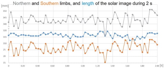
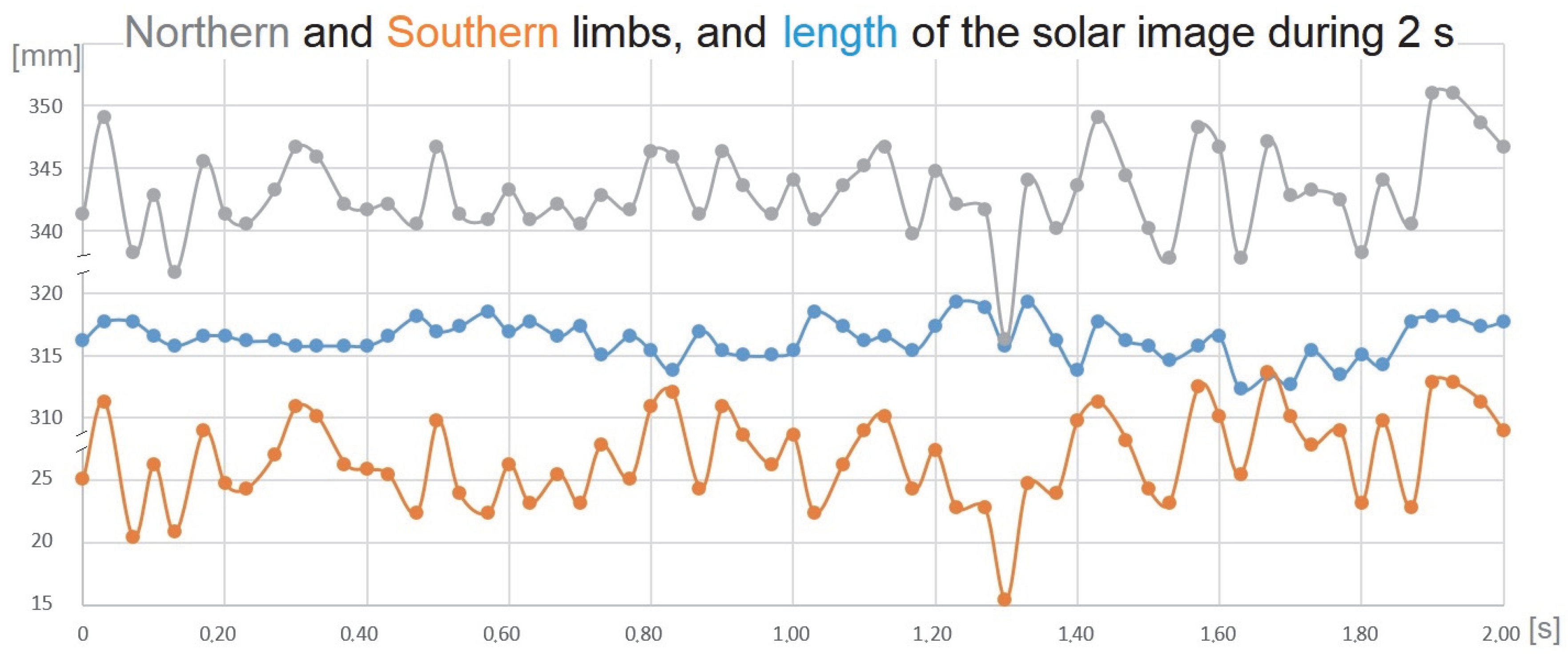
Figure 5.
Position of the Northern and Southern limbs in 61 consecutive frames separated by 1/30 s each, in a 2.00 s video on 29 March 2022 at 13:20:29–31.
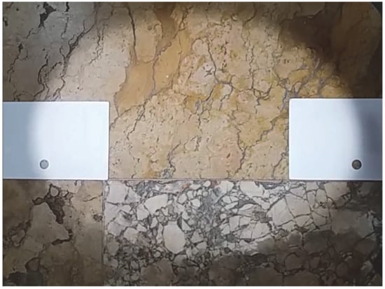
Figure 6.
The 2.00 s frame of the video analyzed in Figure 2. The image was on the yellow marble “Giallo di Verona” after the meridian line. The white cards are posed parallel to the meridian line; on them, we found the inflection points of the two meridian solar limbs.
The lengths of the images of Figure 5 have a spread ±1.5 mm (corresponding to a 9″ viewing), which is much lower than the limbs spreading in phase of ±3.6 mm (22″ of viewing). The average length of the image is 316.3 mm from one to another inflection point, and it corresponds to 1922″ of angular dimension (ephemerides). The positions are defined by the inflection points of the light curves for each frame, along the meridian direction. The camera is a Samsung SM-J500FN (Samsung Digital City [KO], Samsungno 129, Maetan-dong, Yeongtong District, Suwon, Republic of Korea) in VGA 640 × 480 pixels in automatic mode.
4.5. Images with Tiny Clouds
The measured length of the solar diameter along the meridian line has been found to be different in scenarios of thin clouds with cover to a fully clear sky.
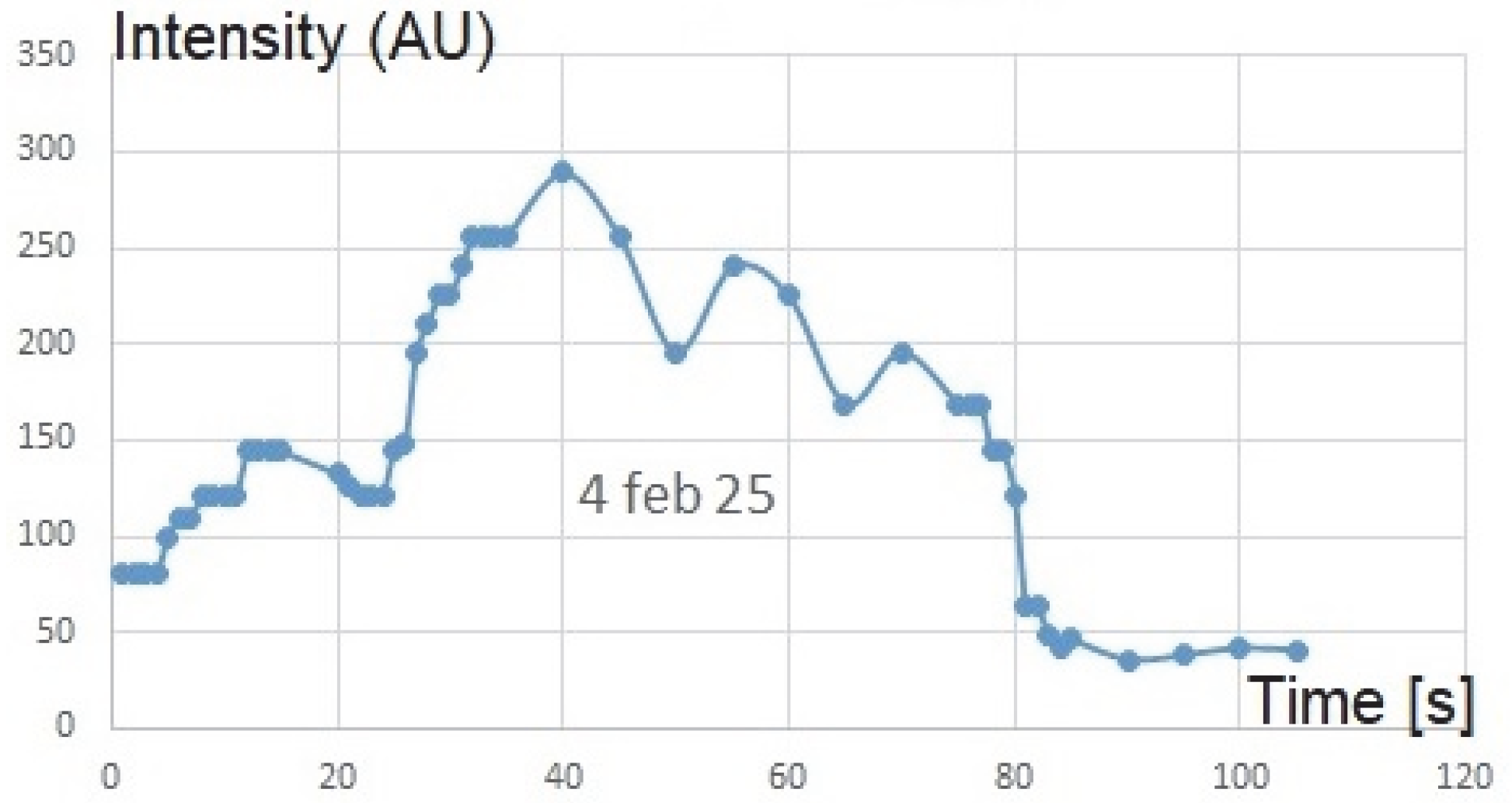
Different cloud coverages (Figure 7) modify the luminosity of the image.
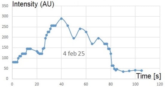
Figure 7.
Photometry during the solar transit of 4 February 2025. (Obtained, before the yellow Veronese marble, from the following video: https://youtu.be/i__e_fgtIas accessed on 4 February 2025). The contrast of the image changes slightly during the transit, determining uncertainties on limbs’ positions under tiny clouds (invisible to our eyes before/after the transit) or full sunlight.
When the luminosity diminishes, the dispersion of the diameter measures increases, and the perceived diameter tends to diminish.
5. Solar Diameters in 1701 and 1702
Francesco Bianchini, around the 1701–1702 winter solstices, performed 11 measurements at the Clementine Gnomon under good weather conditions [3,4]. Ten of them are represented in Figure 8, and one was rejected. (One of the observations near the solstices, on 29 December 1701, resulted in an outlier, with a measured image 42 mm shorter than the ephemerides, while all other measures were in very good agreement with them, with a systematic reduction of 9 mm. Nevertheless, the clear sky conditions of Rome are generally better than the “Sole languido” or “Sole languidissimo” (−/+ clouds’ veil) mentioned in the Manfredi’s report [9]). The mean value of the difference between the observed and calculated diameter (ephemerides with 1920″ solar angular diameter at 1AU) is O-C = −9 mm.
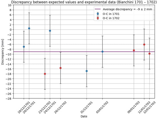
Figure 8.
Ten observations of the solar diameter measured by Bianchini near the winter solstices of 1701 and 1702. The solar diameters are −9 ± 6 mm smaller than the ones calculated with the ephemerides [28]. The standard deviation σ ≈ 6 mm has been assumed as the accuracy of a single measurement and the average m = −9 mm is the systematic difference with respect to the ephemerides for 1701/2.
The measured solar meridian diameters of Bianchini near the end of the solar Maunder minimum (winters 1701–702) are −9 ± 6 mm shorter than the ephemerides (Figure 8), calculated with a solar standard diameter of θ⊙ = 1919.26″, here assumed as θ⊙ = 1920″ (Lamy et al. [31], Quaglia et al. [32]).
6. Comparison Between Bianchini (1702) and Present Data (2018–2025)
The gigantic dimension of the Clementine Gnomon, up to 50 m of focal length, maximizes the signal (1100 mm at the winter solstice) to noise (down to ±1 mm of the image’s turbulent vibration) ratio for the solar image’s measurement.
The dates around the winter solstices from 2018 to 2024 (Figure 9) yielded a meridian solar diameter of −12 ± 8 mm, measured by C. Sigismondi during the IGEA-ZIA campaign. The statistical dispersion is larger than the estimated uncertainties of the single measures. The slightly larger statistical uncertainty is due to having included days with some clouds or veils, and solar image’s motion occurred in the moments of the transits, that are a random effect, while Bianchini [3,4] only observed it under very good conditions.
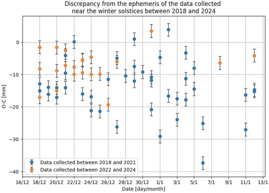
Figure 9.
Seven solstices, with 61 observed datapoints in total. Blue: years 2018–2021, Red: years 2022–2024, all with their uncertainties in mm. The difference with respect to the ephemerides’ observed–calculated “O−C” is represented in mm.
The datapoints under comparison here total 10 from Bianchini (2 winter solstices) and 61 from Sigismondi (7 winter solstices). We chose the data near the winter solstice for their larger relative and absolute accuracy, given the dimensions of the solar images. (The “inaugural” meridian diameter of 6 October 1702 [3] was 415.6 mm long, with the Southern limb coincident with the ephemerides, while the Northern one was −10 mm, so the diameter was −10.6 mm with respect to the ephemerides. Rescaling to the winter solstice this would be −28.6 mm. The choice of using the winter solstices data is for obtaining better relative errors and a largest ratio of image to penumbra (pinhole size). Assuming similar personal equations (the capability to detect the image’s limbs under similar environmental luminosity, in these cases) for Bianchini and Sigismondi, the meridian images have diameters systematically different by 3 mm, since Bianchini underestimated the solar diameter by 9 mm and Sigismondi by 12 mm (Figure 9). The Sun has shrunk by 3 mm or 6″ since then, but the errorbars are ±20″.
Normalizing to the standard angular solar diameter and adjusting for the systematic errors, the averaged winter solstice data of Bianchini are θ⊙ = 1926″ ± 12″, while the modern ones are θ⊙ = 1920″ ± 16″.
The solar diameter’s variation, Δθ⊙ = −6″ ± 20″, is evidently compatible with zero but also with the variations claimed with historical total eclipses. The eclipses of Clavius occurred in Rome in 1567, before the Maunder minimum [33], the one of Halley occurred in England in 1715, which was later [34] analyzed by Eddy and Boornazian [35], and the one over Manhattan (New York) and Providence occurred in 1925 and was analyzed by Dunham et al. [36], along with the eclipse of 1979.
7. Simulating Solar Diameter Variations and the Observations Made in 1655–1736
To study the results obtained by Tovar et al. (2021) on the data published by Manfredi [9], we designed simulations with a gradual change of 1″and 3″ in solar diameter over the years (1655–1715) when the Maunder minimum occurred and a constant value after 1715–1736.
The attribution of a slow positive diameter variation of +1″/80 or +3″/80 years during the Maunder minimum is inspired by the Secchi–Rosa law [37], which anticorrelated the maximum of the solar activity cycle with the minimum diameter measured. The verification of this law continued to inspire the experiments on the solar diameter variations realized in recent years as in the SDS experiment by Egidi et al. [38] and in Picard satellite + ground counterpart (Corbard et al. [39]).
In the simulations, we distinguished two cases: winter and summer:
- Summer. The Gaussian noise is −18″ ± 48″ (from extra-meridian data, since the summer solstice in St. Maria degli Angeli occurs on the figure of Cancer).
Both the systematic shifts (−18″, rather constant along the year, according to our analyses) with respect to the expected values from ephemerides, and the errorbars (±18″ in winter and ±48″ in summer) of the single measures, are the same as those observed in St. Maria degli Angeli.
We simulated 4000 datapoints, as in Manfredi [9], in the two cases winter and summer, obtaining a difference of Δθ⊙ = (0.53 ± 0.43)″ between the last 1000 datapoints (the ones simulating 1715–1736 are with constant solar diameter) and the first 3000 datapoints (1655–1715, are with rising diameter during the Maunder minimum).
The dispersion of the averaged difference Δθ⊙ was obtained through 100 repetitions of 4000 simulated datapoints each (see Figure 10).
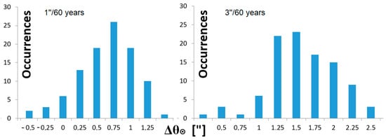
Figure 10.
One hundred simulations of the difference Δθ⊙ between the average diameters of 3000 variating datapoints (+1″/3000) and of 1000 constant datapoints, with the seasonal errorbars observed at the Clementine Gnomon. On the left the solar diameter has been increased by 1″ in 60 years and it remained constant for the following 20 years, on the right side the increment is 3″ in 60 years and constant over the following 20 years. The average differences between these two clusters of data (the last 20 years minus the first 60 years’ averages) have been plotted for hundred occurrences in both cases.
The expected value of this difference Δθ⊙, without the added Gaussian noise, is Δθ⊙ = 0.5″ ± 0.3″.
Changing the ratio of solar diameter variations to +3″ over the first 60 years yr in the timespan of 1655–1715, and constant in the last 20 years, we obtain differences of Δθ⊙ = (1.47 ± 0.46)″, always on 100 repetitions. The expected value in this second case was Δθ⊙ = 1.5″ ± 0.9″.
The distributions of the results are asymmetrical.
The differences of the averages are plotted in the Figure 10 with simulated increments of the solar diameter of 1″ per 60 years or 3″ per 60 years and the following 20 years constant. These simulations have been repeated 100 times times, and we found that there are occurrences very far from the expected values.
For example there are 25% of the occurrences of Δθ⊙ in the range of [0.75–1]″ with the expected value 0.5″ or 15% of the occurrences of Δθ⊙ in the range of [1.75–2]″ with the expected value 1.5″. We deduce from this analysis that a definition of the solar diameter with a sub-arcsecond accuracy, and based on a single random set of 4000 data, cannot be reliable for the structure of the simulated distribution.
The changes in the solar angular diameter, if they occur, are expected to be of the order of ≤1″/century. All instrumental (e.g., the temperature variating the focal length as in the SDS experiment, Egidi et al. [38]) and experimental effects (e.g., refraction, as in Picard experiment, Corbard et al. [39]), or the black drop effect in planetary transits (Schneider et al. [40]), have to be excluded.
Recent experimental data on the solar angular radius have been obtained with ground-based and satellite experiments, such as the Picard satellite with a twin telescope on the ground (θr⊙ = 959.78″ ± 0.19″ Meftah et al. [41]). Recent Baily’s beads analyses in solar eclipses have yielded values of the solar radius (θr⊙ = 959.99″ ± 0.06″ Lamy et al. [31], θr⊙ = 959.95″ ± 0.05″ Quaglia et al. [32]). These values of θr⊙ are up to 0.4″ larger than the standard value of the solar radius at 1AU: θr⊙ = 959.63″ ± 0.02″ (Auwers, [42]). (The solar radius found in the recent aforementioned experiments is 0.8″ larger than the nominal value obtained by the IAU General Assembly 2015 resolution B3 [43] of R⊙ = 695.7 Mm, based on the Rosseland radius at optical depth τ = 2/3 (rounded without errorbars from Haberreiter et al. [44]). This nominal radius yields an angular solar radius of θr⊙ = 959.23″ at 1AU. It should be noted that this nominal value aims to find an agreement between the helioseismological radius and the photometric radii, based on the definition of the solar limb with the inflection point of the radial photometric profiles. R⊙ = 695.7 Mm is a value to be used, with fair precision, in stellar astronomy, based on nominal solar parameters. But the final scope of this study and others regarding solar diameter variations is to better comprehend the physics of the Sun, which may be more complex than expected, being the Sun the only star that we can observe under very high resolution. That’s why we refer to the photospheric solar radius and to its variations.
8. Conclusions and Perspectives
The data of Bianchini 1701–1702 [3,4] and of Sigismondi 2018–2024 were obtained at the winter solstices when the relative uncertainty was lower. After considering the personal equations, the reduced solar diameter was θ⊙ = 1926″ ± 12″ for Bianchini and θ⊙ = 1920″ ± 18″ for Sigismondi, with Δθ⊙ = −6″ ± 20″ occurred after 3 ¼ centuries. There is no possibility to meaningfully constrain our current understanding on the Sun’s evolution better than ±20″ with such instrument.
More than one thousand measures obtained in 2024–2025 with extra-meridian observations (Figure 4) allowed us to better constrain the seasonal errorbars and diameter shifts in S. Maria degli Angeli and to infer the corresponding values for the meridian line of Cassini in S. Petronio, Bologna.
According to these results, we realized opportune realistic simulations to reproduce datasets similar to the one of Manfredi [9] and analyzed by Tovar et al. [10].
With observational errorbars ranging from ±18″ to ±48″ over the year, simulations of 4000 datapoints, reproducing the ones of Manfredi [9], repeated 100 times, yielded averaged diameter variations of Δθ⊙ = (0.4 ± 1.2)″ with respect to a solar diameter increased by +1″ over 80 years.
These differences become Δθ⊙ = (1.6 ± 1.3)″ if the solar diameter varies +3″ during the same examined period.
We conclude that due to a large number of systematic effects and variable biases, no issues regarding the solar diameter variations between the Maunder minimum and the 20 years immediately following can be found with a sub-arcsecond of accuracy, even working with cluster averages.
Author Contributions
C.S. made the measurements, conceived the structure of the paper, and wrote it, A.B. contributed to the statistical analysis, and G.A.B. contributed to Section 4.4. All authors have read and agreed to the published version of the manuscript.
Funding
This research received no external funding.
Data Availability Statement
The data on meridian transits observed in St. Maria degli Angeli have been published on a daily basis on the dedicated Youtube channel Sigismondi Costantino https://www.youtube.com/channel/UCe18v3EZ8w2qmd8jW6mYV5w/videos (accessed on 4 June 2025).
Acknowledgments
Costantino Sigismondi wants to gratefully remember Mons. Giuseppe Blanda (1937–2022), who supported his observations by publishing his reports in the official website of the Basilica, and John L. Heilbron (1934–2023), who inspired the study of the Clementine Gnomon with his masterpiece “The Sun in the Church” (1999). Thanks also to Rev. Father Rafael Pascual LC, who has included the meridian line of S. Maria degli Angeli in the course of History of Astronomy in the Masters of Science and Faith of Regina Apostolorum University since 2004. Thanks to Rev. Don Francesco Bianchini, Don Tingy Pietro Cai, and Rev. Fr. Michael Asare Appau for their patience exercised… at lunch time! Thanks to Ilaria Caruso, Paola Giudizio and Linda Salvati. Thanks to Mons. Renzo Giuliano, Don Franco Cutrone, and Don Pietro Guerini: the rectors of the Basilica of S. Maria degli Angeli since 1999, when these astronomical observations started. Thanks to Father David Netzereab-Teclemichael Hagos O. Cist., for the insights on the mystic of science, discussed during the observations.
Conflicts of Interest
The authors declare no conflicts of interest.
References
- Heilbron, J.L. The Sun in the Church; Harvard Universtiy Press: Cambridge, MA, USA, 2001. [Google Scholar]
- Heilbron, J.L. The Incomparable Monsignor: Francesco Bianchini’s World of Science, History, and Court Intrigue; Oxford University Press: Oxford, UK, 2022. [Google Scholar]
- Bianchini, F. De Nummo et Gnomone Clementino, Romae. 1703. Available online: https://archive.org/details/dekalendarioetcy00bian/ (accessed on 4 June 2025).
- Bianchini, F. Correspondance; Fondo Bianchini; Biblioteca Vallicelliana: Roma, Italy, 1702. [Google Scholar]
- Sigismondi, C. Lo Gnomone Clementino, Roma (2009). Gerbertus 2014, 7, 3–80. [Google Scholar]
- Sigismondi, C. Earth’s Obliquity and Stellar Aberration Detected at the Clementine Gnomon (Rome, 1703). Phys. Sci. Forum 2021, 2, 49. [Google Scholar] [CrossRef]
- Danti, E. Usus et Tractatio Gnomoni Magni, Bononiae: Apud Ioannem Rossium. 1576. Available online: https://opac.museogalileo.it/imss/resourceXsl?uri=365759 (accessed on 6 June 2025).
- Cassini, G.D. La Meridiana del Tempio di S. Petronio: Tirata, e Preparata per le Osseruazioni Astronomiche L’anno 1655: Riuista, e Restaurata L’anno 1695, in Bologna: Per L’erede di Vittorio Benacci (1695). Available online: https://archive.org/details/lameridianadelte00cass (accessed on 4 June 2025).
- Manfredi, E. Opera Omnia, 3: De Gnomone Meridiano Bononiensi; Lelio dalla Volpe: Bologna, Italy, 1736. [Google Scholar]
- Tovar, I.; Aparicio, A.J.P.; Carrasco, V.M.S.; Gallego, M.C.; Vaquero, J.M. Analysis of Solar Diameter Measurements Made at the Basilica of San Petronio During and After the Maunder Minimum. Astrophys. J. 2021, 912, 122. [Google Scholar] [CrossRef]
- da Passano, C.F.; Monti, C.; Mussio, L. La Meridiana Solare del Duomo di Milano, Verifica e Ripristino Nell’anno 1976; Veneranda Fabbrica del Duomo di Milano: Milan, Italy, 1977. [Google Scholar]
- Galilei, G. Istoria e Dimostrazioni Intorno alle Macchie Solari; Accademia dei Lincei: Roma, Italy, 1613. [Google Scholar]
- Available online: https://articles.adsabs.harvard.edu/pdf/1844AN.....21..233S (accessed on 4 June 2025).
- Maunder, E.W. A prolonged sunspot minimum. In Knowledge: An Illustrated Magazine of Science; #247—Knowledge; A Monthly Record of Science v.17 1894—Full View; HathiTrust Digital Library: Champaign, IL, USA, 1894; Volume 17, pp. 173–176. Available online: https://babel.hathitrust.org/cgi/pt?id=uc1.c2834645&view=1up&seq=247 (accessed on 4 June 2025).
- Maunder, E.W. The prolonged sunspot minimum, (1645–1715). J. Br. Astron. Assoc. 1922, 32, 140–145. [Google Scholar]
- Usoskin, I.G. A history of solar activity over millennia. Living Rev. Sol. Phys. 2023, 20, 2. [Google Scholar] [CrossRef]
- Whitehouse, D. Il Sole Una Biografia; Mondadori: Milano, Italy, 2007. [Google Scholar]
- Carrasco, V.M.S.; Vaquero, J.M. Sunspot Observations During the Maunder Minimum from the Correspondence of John Flamsteed. Sol. Phys. 2016, 291, 2493–2503. [Google Scholar] [CrossRef]
- Carrasco, V.M.S.; Vaquero, J.M.; Gallego, M.C.; Muñoz-Jaramillo, A.; de Toma, G.; Galaviz, P.; Arlt, R.; Pavai, V.S.; Sánchez-Bajo, F.; Álvarez, J.V.; et al. Sunspot Characteristics at the Onset of the Maunder Minimum Based on the Observations of Hevelius Astrophys. Astrophys. J. 2019, 886, 18. [Google Scholar] [CrossRef]
- Carrasco, V.M.S.; García-Romero, J.M.; Vaquero, J.M.; Rodríguez, P.G.; Foukal, P.; Gallego, M.C.; Lefèvre, L. The Umbra–Penumbra Area Ratio of Sunspots During the Maunder Minimum. Astrophys. J. 2018, 865, 88. [Google Scholar] [CrossRef]
- Carrasco, V.M.S.; Gallego, M.C.; Arlt, R.; Vaquero, J.M. On the Use of Naked-Eye Sunspot Observations During the Maunder Minimum. Astrophys. J. 2020, 904, 60. [Google Scholar] [CrossRef]
- Shapley, H. (Ed.) Climatic Change. Evidence, Causes, and Effects; Harvard University Press: Cambridge, MA, USA, 1953. [Google Scholar]
- CNES Toulouse. Sun and Climate. 1980. Available online: https://catalogue.bnf.fr/ark:/12148/cb34658419f (accessed on 4 June 2025).
- Penza, V.; Berrilli, F.; Bertello, L.; Cantoresi, M.; Criscuoli, S.; Giobbi, P. Total Solar Irradiance During the Last Five Centuries. Astrophys. J. 2022, 987, 84. [Google Scholar] [CrossRef]
- Sullivan, W.; Thorp, M.; Tovar, G.; Look, J. Modern Observations Using the 1702 Meridian Line of the Basilica of Santa Maria Degli Angeli e dei Martiri (Rome). 2016. Available online: https://archive.sundialsoc.org.uk/wp-content/uploads/Bulletin-29iii-Sullivan.pdf (accessed on 4 June 2025).
- Sigismondi, C. Pinhole giant meridian lines: A review on ancient data retrieval and modern observations (IGEA-ZIA campaign). Gerbertus 2022, 16, 29. [Google Scholar]
- Sigismondi, C. Measuring the angular solar diameter using two pinholes. Am. J. Phys. 2002, 70, 1157. [Google Scholar] [CrossRef]
- Espenak, F. Earth at Perihelion and Aphelion: 1701 to 1800. Available online: https://astropixels.com/ephemeris/perap/perap1701.html (accessed on 13 February 2025).
- Catamo, M.; Lucarini, C. Il Cielo in Basilica; Arpa-Agami: Roma, Italy, 2012. [Google Scholar]
- Schiavo, A. La Meridiana di S. Maria Degli Angeli; Istituto Poligrafico e Zecca Dello Stato: Roma, Italy; Libreria dello Stato: Roma, Italy, 1993. [Google Scholar]
- Lamy, P.; Prado, J.-Y.; Floyd, O.; Rocher, P.; Faury, G.; Koutchmy, S. A Novel Technique for Measuring the Solar Radius from Eclipse Light Curves—Results for 2010, 2012, 2013, and 2015. Sol. Phys. 2015, 290, 2617–2648. [Google Scholar] [CrossRef]
- Quaglia, L.; Irwin, J.; Emmanouilidis, K.; Pessi, A. Estimation of the Eclipse Solar Radius by Flash Spectrum Video Analysis. Astrophys. J. 2021, S256, 36. [Google Scholar] [CrossRef]
- Clavius, C. Commentarius in Sphaeram; Ex Officina Dominici Basae Romae: Rome, Italy, 1581. [Google Scholar]
- Halley, E. Philosophical Transactions (1683–1775); Royal Society: London, UK, 1717; Volume 29, pp. 245–262. [Google Scholar]
- Eddy, J.; Boornazian, A.A.; Clavius, C. Shrinking Sun. Sky Telesc. 1980, 60, 10. [Google Scholar]
- Dunham, D.W.; Sofia, S.; Fiala, A. Observations of a probable change in the solar radius between 1715 and 1979. Science 1980, 210, 1234. [Google Scholar] [CrossRef] [PubMed]
- Rosa, P. Intorno ad una identità di periodi di fenomeni fotosferici e magnetici in connessione con il moto proprio del Sole. Mem. Degli Spettrosc. Italiani 1874, 3, 67. [Google Scholar]
- Egidi, A.; Caccin, B.; Sofia, S.; Heaps, W.; Hoegy, W.; Twigg, L. High-Precision Measurements of the Solar Diameter and Oblateness by the Solar Disk Sextant (SDS) Experiment. Sol. Phys. 2006, 235, 407–418. [Google Scholar] [CrossRef]
- Corbard, T.; Ikhlef, R.; Morand, F.; Meftah, M.; Renaud, C. On the importance of astronomical refraction for modern solar astrometric measurements. Mon. Not. R. Astron. Soc. 2019, 483, 3865–3877. [Google Scholar] [CrossRef]
- Schneider, G.; Pasachoff, J.M.; Golub, L. The black drop effect. Sky Telesc. 2012, 123, 8. [Google Scholar]
- Meftah, M.; Corbard, T.; Irbah, A.; Ikhlef, R.; Morand, F.; Renaud, C.; Hauchecorne, A.; Assus, P.; Borgnino, J.; Chauvineau, B.; et al. Ground-based measurements of the solar diameter during the rising phase of solar cycle 24. Astron. Astrophys. 2014, 569, A60. [Google Scholar] [CrossRef]
- Auwers, A. Der Sonnendurchmesser und der Venusdurchmesser nach den Beobachtungen an den Heliometern der deutschen Venus-Expeditionen. Astron. Nachrichten 1891, 128, 361. [Google Scholar] [CrossRef]
- IAU Inter-Division A-G Working Group on Nominal Units for Stellar & Planetary Astronomy. Resolution B3 on Recommended Nominal Conversion Constants for Selected Solar and Planetary Properties. 2015. Available online: https://arxiv.org/pdf/1510.07674 (accessed on 4 June 2025).
- Haberreiter, M.; Schmutz, W.; Kosovichev, A.G. Solving the Discrepancy Between the Seismic and Photospheric Solar Radius. Astrophys. J. Lett. 2008, 675, L53. [Google Scholar] [CrossRef]


Disclaimer/Publisher’s Note: The statements, opinions and data contained in all publications are solely those of the individual author(s) and contributor(s) and not of MDPI and/or the editor(s). MDPI and/or the editor(s) disclaim responsibility for any injury to people or property resulting from any ideas, methods, instructions or products referred to in the content. |
© 2025 by the authors. Licensee MDPI, Basel, Switzerland. This article is an open access article distributed under the terms and conditions of the Creative Commons Attribution (CC BY) license (https://creativecommons.org/licenses/by/4.0/).