Flare Set-Prediction Transformer: A Transformer-Based Set-Prediction Model for Detailed Solar Flare Forecasting

Abstract

Solar flare prediction models typically use classification, predicting only the probability of categorized events within a time window. This misses critical information, such as how many flares occur, their precise timings, and their intensities. To address this, we propose a paradigm shift to set prediction, directly forecasting a variable-sized set of flare events with detailed characteristics. We demonstrate this approach with FSPT (Flare Set-Prediction Transformer), a transformer-based model adapted from object detection principles. FSPT predicts sets containing individual flare start, peak, and end time offsets, as well as peak X-ray intensity. This work presents the set-prediction framework and the FSPT model, showing its potential for more informative flare forecasting.

1. Introduction

Solar flares, which are potent bursts of radiation driven by the release of magnetic energy in the solar atmosphere [1], represent a significant component of space weather capable of disrupting terrestrial and space-borne technological systems. Accurate and timely prediction of these events is therefore crucial for mitigating their adverse impact.

Historically, flare prediction relied on statistical methods that linked flare occurrences to observable parameters like regional magnetic properties [2], often employing probabilistic frameworks such as Bayesian inference [3] or Poisson statistics [4]. Subsequently, machine learning (ML) techniques gained prominence, with various algorithms applied to flare forecasting, including support vector machines [5], random forests [6], and comparative studies assessing multiple approaches [7]. In recent years, deep learning has become a principal methodology, demonstrating considerable success. Numerous studies have leveraged diverse datasets and sophisticated model architectures. However, the predominant approach in much of this prior work formulates flare prediction primarily as a classification task. In this paradigm, the goal is typically to predict the probability of a specific category of event occurring within a predefined future time window. For instance, the Deep Flare Net (DeFN) model developed by [8,9] utilized a deep neural network to calculate the probability of flares (e.g., ≥M-class or ≥C-class) occurring within the next 24 h for each active region, framed as a binary classification problem. Similarly, numerous studies have employed Convolutional Neural Networks (CNNs) [10,11,12,13,14] and Long Short-Term Memory (LSTM) networks [15,16] to predict flare likelihoods within predefined categories and time windows.

More recently, Pandey et al. [17] utilized models like ResNet34 and MobileNet, which were trained on active-region patches, to predict M-class flares, again focusing on classification and evaluating performance using metrics derived from classification contingency tables (TSS and HSS).

While these classification-based approaches have achieved notable improvements in predictive skill, as often measured by metrics like TSS [9,10,17,18], they suffer from inherent limitations imposed by the classification framework itself. Specifically, they cannot provide crucial details beyond the probability of a categorized event, and there are crucial aspects that remain unaddressed. First, the number of distinct flares that will occur is unknown. Second, the precise location of each flare has not been determined. Third, the peak soft X-ray intensity of each individual flare is yet to be ascertained. Fourth, the specific onset, peak, and end times for each flare event have not been specified.

To overcome these limitations, we propose what we consider a paradigm shift within the application of machine learning to solar flare prediction: reframing the task as a set-prediction problem.

In set prediction, the model’s objective is to directly output a variable-sized set of entities, where each entity possesses specific attributes. This formulation naturally aligns with the physical reality of solar flares, where multiple distinct events, each with unique characteristics (timing, intensity, location, etc.), can occur within a forecast period or originate from the same active region. By adopting set prediction, we can design models capable of answering the detailed questions left unaddressed by classification approaches.

The set-prediction framework is conceptually analogous to object detection in computer vision, where the goal is to output a set of bounding boxes, each associated with a class label and confidence score. Influential object detection models like DETR (DEtection TRansformer, [19]) have successfully employed transformers for direct set prediction, eliminating the need for hand-crafted components like anchor boxes and non-maximum suppression (NMS). Given these parallels—predicting a variable number of ‘objects’ (flares) with associated properties—the architectural principles of DETR provide a relevant basis for our task. However, solar flare prediction differs significantly from typical object detection: our ‘objects’ are temporal events rather than spatial entities within a single image, and their key attributes are time offsets and intensity, not bounding-box coordinates. Therefore, while inspired by DETR, substantial technical adaptations are necessary. These include designing novel prediction heads specifically for flare temporal offsets and peak X-ray intensity, formulating a set-based loss function tailored to these physical characteristics, and defining a matching strategy based on temporal and intensity similarity rather than spatial overlap to meet the unique demands of comprehensive solar flare forecasting.

As a demonstration of this new paradigm, we introduce FSPT, a transformer-based model designed for flare set prediction. This paper is structured as follows. Section 2 details the dataset construction, including the source data, our novel label-generation process for set prediction, and the data-splitting strategy. Section 3 presents the FSPT model architecture, the set-based loss function, the matching strategy used during training, and the overall training pipeline. Section 4 discusses the evaluation methodology, including the inference pipeline, appropriate evaluation metrics (AP and F1), and presents the quantitative results. Finally, Section 5 concludes this paper and outlines directions for future work.

2. Dataset

The foundation of our study is a curated dataset derived from the comprehensive collection of solar active-region magnetograms presented by Boucheron et al. [20]. We utilize the core image data from this source and introduce a novel labeling scheme tailored to our set-prediction paradigm for solar flares.

The base dataset consists of consistently sized, $224\times 224$-pixel, single-channel Line-of-Sight (LOS) photospheric magnetogram images of solar active regions (ARs). These images originated from the Helioseismic and Magnetic Imager (HMI) instrument [21] aboard the National Aeronautics and Space Administration’s (NASA) Solar Dynamics Observatory (SDO). The choice of this dataset format over alternatives, such as the Space-Weather HMI Active-Region Patches (SHARPs) [22], was primarily driven by the fixed-image dimensions ($224\times 224$) provided by Boucheron et al. [20]. Variable dimensions, as found in SHARPs, are incompatible with standard deep learning architectures like the ResNet backbone used in FSPT, which typically require consistent input sizes. The Boucheron et al. dataset provides a minimally processed, user-configurable resource focused solely on ARs, alleviating the need for extensive data downloading and curation specific to these regions.

2.1. Label Generation for Set Prediction

While the base dataset provides the essential magnetogram inputs, its original labeling might focus on classification tasks. To facilitate our novel set-prediction approach, we implement a tailored label-generation process. The process begins with identifying the precise capture timestamp and corresponding NOAA active-region (AR) number for each $224\times 224$ HMI LOS magnetogram image in our selected subset. Subsequently, the official NOAA Geostationary Operational Environmental Satellite (GOES) flare-event list is queried to retrieve all recorded flare events associated with the identified AR number. A crucial temporal-filtering step follows, where associated flares are selected based on their relationship to the magnetogram’s capture time; specifically, flares are included if they were either already in progress at the time of the image capture or initiated within the subsequent 48-h period, a duration commonly used in operational forecasting. This inclusion of ongoing flares is motivated by the value in forecasting their remaining evolution (peak time, end time, and peak intensity), even post-onset. Finally, for each flare passing this filter, its key characteristics (start, peak, end times, and peak X-ray intensity) are extracted. Time offsets relative to the image’s capture timestamp are calculated for the start, peak, and end times. The resulting label assigned to each input magnetogram is thus a set (represented as a list) containing zero or more flare instances, where each instance is defined by a tuple $(\Delta t_{\mathrm{start}}, \Delta t_{\mathrm{peak}}, \Delta t_{\mathrm{end}}, I_{\mathrm{peak}})$, comprising the temporal offsets and the numerical peak soft X-ray flux value (in W/m²). This process transforms the task from simple classification to predicting a variable-sized set of future or ongoing flare events with detailed temporal and intensity information for each one.

2.2. Dataset-Splitting Strategy

Properly splitting the dataset into training and test sets is critical to ensure reliable model evaluation and prevent overly optimistic performance estimates due to data leakage. We address two primary concerns, as outlined below.

Preventing Data Leakage: HMI images are captured at a high cadence (magnetograms are available frequently), leading to high similarity between consecutive images of the same AR. Naively splitting individual images randomly would lead to near-identical samples appearing in both the training and test sets, a form of data leakage that inflates performance metrics. To mitigate this, we adopt a group-based splitting strategy. All magnetogram samples belonging to a single, unique NOAA AR number are treated as an indivisible group. Each group is assigned entirely to either the training set or the test set, ensuring that temporally correlated data from the same physical region do not span across the split.

Maintaining Distributional Similarity: Simply grouping by AR is insufficient, as it might lead to skewed distributions of flare events between the training and test sets. It is crucial that both sets reflect similar statistical properties regarding flare occurrences. Specifically, we aim to balance both the overall ratio of ground-truth flare instances to the total number of magnetogram samples and the relative proportions of different flare-intensity classes (A, B, C, M, and X) within each set. Significant discrepancies in these distributions could bias model training or lead to unreliable performance evaluation on the test set.

To achieve a balanced split while adhering to the AR grouping constraint, we employ a simulated annealing optimization algorithm. This probabilistic technique iteratively assigns AR groups to either the training or test set. Starting from a random partition (e.g., targeting a 90%/10% train/test split by AR group count), the algorithm proposes moves of AR groups between sets. Moves that reduce the discrepancy between the target distributions (flare-to-sample ratio and class ratios) in the two sets are accepted. Moves that increase the discrepancy are accepted with a probability that decreases over time (controlled by a “temperature” parameter), allowing the algorithm to escape local minima and find a near-optimal partition that minimizes the statistical differences between the training and test sets.

The simulated annealing process results in a final dataset split that allocates AR groups to the training and test sets. The training set comprises 849,134 magnetogram samples, while the test set contains 94,322 samples, approximating a 90%/10% split in terms of sample count (although the split is primarily based on AR groups). Crucially, this division achieves a close balance in the critical statistical properties between the two sets, validating the effectiveness of the allocation strategy.

The proportion of samples associated with at least one flare (i.e., having a non-empty target set) is highly comparable: 32.63% in the training set (277,050 out of 849,134 samples) and 31.28% in the test set (29,505 out of 94,322 samples). Furthermore, the distribution of flare-intensity classes among the total recorded target flares (787,416 in training; 87,262 in test) is well preserved across the split. As shown in

Table 1. Comparison of key statistics between the training and test sets after simulated annealing allocation. Percentages for flare classes are relative to the total number of target flares within each set.

Statistic	Training Set	Test Set
Total Samples	849,134	94,322
Samples with Flares (%)	32.63%	31.28%
Total Target Flares	787,416	87,262
Flare-Class Distribution:
A-Class (%)	0.10%	0.17%
B-Class (%)	28.73%	29.45%
C-Class (%)	64.09%	63.16%
M-Class (%)	6.59%	6.55%
X-Class (%)	0.49%	0.67%

, the relative frequencies of different flare classes are maintained: C-class flares constitute 64.09% of training-set flares and 63.16% of test-set flares; M-class flares represent 6.59% and 6.55%, respectively; B-class flares 28.73% and 29.45%; X-class flares 0.49% and 0.67%; and A-class flares 0.10% and 0.17%. This statistical similarity ensures that the model is trained and evaluated on representative data distributions.

We opt for only training and test sets primarily because the AR grouping strategy significantly reduces the number of independent data points, making a separate validation set less practical. Model selection and hyperparameter tuning are consequently performed using cross-validation within the designated training set during the development phase.

2.3. Data Processing and Augmentation

Input magnetograms undergo initial preprocessing. Input images are initially processed such that pixel values are scaled to the [0, 1] range. Subsequently, Z-score normalization is applied using the global mean (0.017047) and standard deviation (0.017998) computed from the entire training set. This standardization ensures a consistent input distribution for the model.

Given the inherent similarity among consecutive magnetograms within each AR group, the effective diversity of the training data is limited. To enhance the model’s ability to generalize to unseen data and mitigate the risk of overfitting, particularly relevant for our dataset size, we apply several data augmentation techniques randomly during training only, after the initial normalization step. These include random horizontal flips and random vertical flips (each applied with a probability of 0.5), random 90-degree rotations (0, 90, 180, or 270 degrees), and the application of Gaussian noise (mean = 0.0; std = 0.2; applied with probability 0.5). The standard deviation for the noise is chosen to provide moderate regularization on the normalized data (which has a standard deviation close to 1), aiming to improve model robustness against overfitting. These transformations artificially increase the variety of the training samples without altering the associated flare labels.

3. Model

Our approach adapts the DETR framework [19] for solar flare prediction from the $224\times 224$ HMI magnetogram images. The core components include a modified ResNet backbone, a transformer encoder–decoder, prediction heads tailored for flare characteristics, a Hungarian matching strategy to align predictions with ground-truth flares, and a set-based loss function.

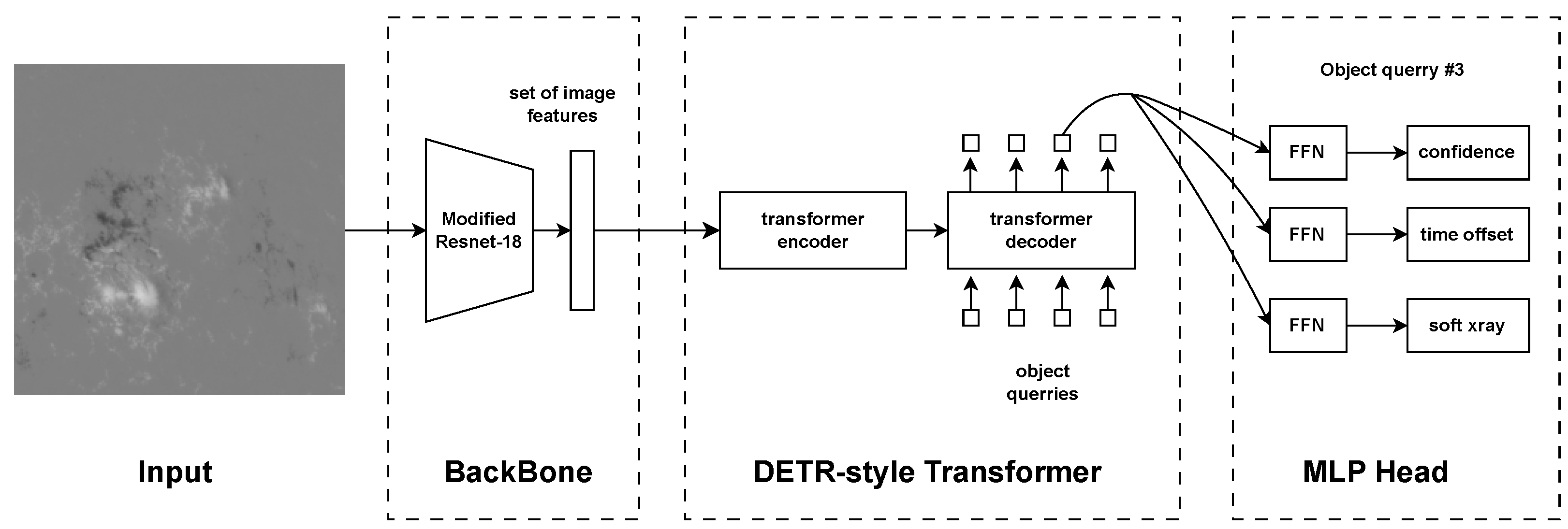
3.1. Model Architecture

The FSPT model architecture sequentially processes the input image through a convolutional backbone, a transformer network, and specialized prediction heads. A schematic overview of the architecture is provided in Figure 1. The key architectural hyperparameters are summarized in

Table 2. Key architectural hyperparameters for the FSPT model.

Hyperparameter Description	Value
Transformer hidden dimension	256
Number of multi-head attention heads	8
Number of transformer encoder layers	3
Number of transformer decoder layers	3
Dimension of transformer feed-forward networks	2048
Dropout rate within transformer layers	0.1
Number of object queries input to decoder	100
Confidence head output dimension	64
Time/X-ray head MLP hidden dimension	128
Time/X-ray head MLP layers	2

.

We employ a ResNet-18 architecture [23] as the backbone. Compared to deeper alternatives like ResNet-50, ResNet-18 offers a reduced parameter count, which helps mitigate the risk of overfitting given the specific characteristics and size of our dataset. Initial experiments indicated that deeper backbones like ResNet-50 did not yield significant performance gains and showed a higher tendency to overfit. To process the single-channel HMI magnetograms, the backbone’s initial convolutional layer is modified to accept a single-input channel. Pre-trained ImageNet weights are used for initialization where applicable. The final classification layer of the ResNet-18 is removed, and the feature map from the last residual block serves as input to the transformer. The backbone can be fine-tuned during training. Following the backbone, a DETR-style transformer architecture [19,24] with an encoder–decoder structure processes the extracted features. A 1 × 1 convolution reduces the feature dimension before feeding the features into the encoder. Fixed sinusoidal positional encodings are added to the features to provide spatial information. The encoder uses multi-head self-attention and feed-forward networks (FFNs) with ReLU activation, applying layer normalization before each sub-layer (pre-norm) to refine the image features, producing a context-aware memory.

The decoder then takes this memory as input. A crucial component of this DETR-style approach is the use of a fixed-size set of N (in our case, $N=100$) learnable embeddings known as object queries. These object queries are a central concept in DETR-like architectures [19]. They are not derived directly from the input image but are learned during training. Think of them as N independent "slots" or "probes". In the context of FSPT, each object query can be interpreted as representing a potential flare candidate. The model learns to specialize these queries during training to detect different types or aspects of potential flares.

The decoder processes these queries through multiple layers. Within each layer, masked self-attention allows the queries to interact and refine their understanding relative to each other (e.g., avoiding duplicate predictions). Critically, cross-attention layers allow each object query (each potential flare candidate) to attend to different parts of the encoder’s image feature memory. This enables each query to gather the specific visual evidence from the magnetogram needed to predict the characteristics (timing and intensity) of a potential flare or to determine that no significant flare corresponds to that query. After passing through the decoder layers and feed-forward networks (FFNs), each of the N object queries produces a final output embedding.

This mechanism is key to set prediction; although there are always N queries and thus N raw outputs, the model learns to associate a specific prediction (confidence scores, time offsets, and intensity) with each query. Queries that do not correspond to a real flare are effectively assigned a "no object" or background status (typically indicated by a low confidence score from the corresponding prediction head). This allows the model to output a variable number of detected flares (from 0 up to N), based on which “candidate slots” successfully find evidence, without needing post-processing steps like non-maximum suppression (NMS), which are common in other object detection methods.

Finally, the output embeddings from the decoder are fed into three separate prediction heads, adapted for the flare prediction task: a single linear layer for the confidence head (predicting the confidence score); two MLPs, each with one hidden layer, for the novel time offset head (predicting start, peak, and end time offsets relative to the image timestamp); and the novel X-ray intensity head (predicting the normalized base-10 logarithm of the peak X-ray intensity). This specific configuration of prediction heads differs from the original DETR, which uses a linear layer for class prediction but a deeper three-layer MLP for bounding-box regression, representing our adaptation for the flare forecasting task.

3.2. Matching Strategy

A key aspect of FSPT is matching the fixed-size set of N predictions to the variable-sized set of M ground-truth flares within an image. This bipartite matching, performed during training, replaces the need for complex post-processing like non-maximum suppression (NMS) used in traditional object detectors.

Following the original DETR methodology, we employ the Hungarian algorithm [25] to find the optimal one-to-one assignment $\widehat{\sigma }$ between the predictions and ground-truth flares that minimizes a total matching cost. The algorithm operates on a pairwise cost matrix $C\in {\mathbb{R}}^{N\times M}$, where each element $C_{i,j}$ represents the cost of matching the i-th prediction with the j-th ground-truth flare.

While the core mechanism of bipartite matching via the Hungarian algorithm is adopted from DETR, the definition of the matching cost $C_{i,j}$ is tailored specifically for our solar flare prediction task. Unlike DETR, which typically uses costs based on class probability and bounding-box Intersection over Union (IoU), our cost is a weighted sum of three components designed to measure the similarity between predicted and ground-truth flare characteristics: a confidence cost derived from the predicted confidence score; a time offset cost representing the L1 distance between the predicted and ground-truth time offsets; and an X-ray intensity cost reflecting the L1 distance between the predicted and ground-truth (normalized) base-10 logarithm of the X-ray intensities. Defining this physically meaningful, non-spatial cost metric is crucial for applying bipartite matching to temporal flare events. Distinct weights control the influence of each component in the matching cost.

The Hungarian algorithm finds the assignment minimizing the sum of costs for matched pairs. The resulting matches dictate which predictions are treated as positive examples (contributing to all loss terms) and which are negative/background examples (contributing only to the confidence loss) during the loss calculation (Section 3.3).

3.3. Loss Function

Once the optimal matching $\widehat{\sigma }$ between the predictions and ground-truth flares is established using the Hungarian algorithm (Section 3.2), the training of FSPT utilizes a set-based loss function characteristic of DETR models. This loss is computed globally by comparing the set of N predictions against the set of M ground-truth flares, informed by the matching outcome.

The total loss is calculated as a weighted sum of three components: a confidence loss and regression losses. For the confidence loss ${\mathcal{L}}_{\mathrm{conf}}$, we employ the focal loss [26] to effectively handle the class imbalance between the numerous background queries (unmatched predictions) and the fewer foreground queries (matched predictions) by down-weighting easily classified examples. It is calculated over all N query predictions.

The regression losses utilize the L1 loss (Mean Absolute Error) and are calculated solely for the matched prediction–ground-truth pairs identified by $\widehat{\sigma }$. These losses, specifically formulated for flare properties, encompass both a time offset loss (${\mathcal{L}}_{\mathrm{time}}$) applied to the predicted triplet of time offsets (${\widehat{t}}_{\widehat{\sigma }\left(i\right)}$ vs. $t_i$), and an X-ray intensity loss (${\mathcal{L}}_{\mathrm{xray}}$) applied to the predicted normalized log10 intensity (${\widehat{I}}_{\widehat{\sigma }\left(i\right)}^{\prime }$ vs. $I_i^{\prime }$).

The total loss ${\mathcal{L}}_{\mathrm{total}}$ is then computed as a weighted sum:

$${\mathcal{L}}_{\mathrm{total}}={\lambda }_{\mathrm{conf}}{\mathcal{L}}_{\mathrm{conf}}+{\lambda }_{\mathrm{time}}{\mathcal{L}}_{\mathrm{time}}+{\lambda }_{\mathrm{xray}}{\mathcal{L}}_{\mathrm{xray}}$$

where ${\lambda }_{\mathrm{conf}},{\lambda }_{\mathrm{time}},{\lambda }_{\mathrm{xray}}$ are the hyperparameters controlling the relative weight of each component. In this formulation, ${\mathcal{L}}_{\mathrm{conf}}$ represents the focal loss computed over all N predictions, while ${\mathcal{L}}_{\mathrm{time}}$ and ${\mathcal{L}}_{\mathrm{xray}}$ denote the L1 losses calculated only for the matched pairs, penalizing errors in predicted time offsets and normalized log10 X-ray intensity, respectively.

Hyperparameters (the $\lambda$ values) control the relative weight of each loss component. Auxiliary losses can be computed from intermediate decoder layers to aid convergence, with the final loss being an average across all layers.

3.4. Training Pipeline

The training process for FSPT closely follows the end-to-end methodology established by DETR, integrating the model architecture (Section 3.1), matching strategy (Section 3.2), and loss function (Section 3.3) described previously. The pipeline, implemented in the training script, proceeds for each training batch as outlined below.

During training, input magnetograms are processed in batches. Each individual magnetogram within a batch undergoes a forward pass through the FSPT model—encompassing the ResNet backbone, transformer encoder–decoder, and prediction heads—yielding a set of N predictions $({\widehat{z}}_i,{\widehat{t}}^{\left(i\right)},{\widehat{I}}^{\prime \left(i\right)})$ per image, where $\widehat{t}$ represents the predicted time offsets and ${\widehat{I}}^{\prime }$ represents the predicted base-10 logarithm of density with normalization.

Next, the Hungarian algorithm determines the optimal bipartite matching $\widehat{\sigma }$ between these N predictions and the M ground-truth flares for each image, utilizing the cost function defined in Section 3.2. Subsequently, the set-based loss (Section 3.3) is computed using these matches; this involves calculating the focal loss for confidence across all N predictions and the L1 regression losses for the time offsets and X-ray intensity exclusively for the matched pairs. Finally, the total loss is backpropagated through the network, and the model parameters are updated via the AdamW optimizer [27]. Weight decay (L2 regularization, set to 3 × 10⁻⁴) is applied to mitigate overfitting. Learning rate scheduling, using the OneCycleLR scheduler [28], is employed throughout training, and gradient clipping is used to prevent potential gradient explosion and enhance training stability.

To accelerate convergence and leverage knowledge learned from large-scale datasets, we initialize parts of our model with pre-trained weights. The ResNet-18 backbone is initialized using weights pre-trained on ImageNet [29], adapting the first layer for the single-channel input (as described in Section 3.1). Furthermore, the transformer encoder and decoder are initialized with weights from a DETR model pre-trained on object detection tasks (e.g., COCO dataset [30]). Although fine-tuning is essential for adapting to the solar flare prediction task, this initialization can potentially leverage general sequence-processing capabilities learned from large-scale object detection datasets, accelerating convergence on our specific task. The loading and potential modification of pre-trained weights are handled within the model initialization procedure. Data-augmentation techniques (Section 2.3) and early stopping based on the validation loss (monitored via cross-validation on the training set) are employed to mitigate overfitting and find the optimal model checkpoints.

4. Evaluation and Discussion

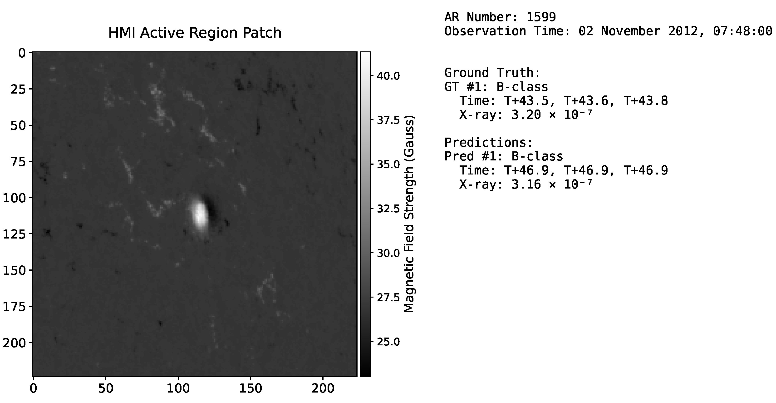
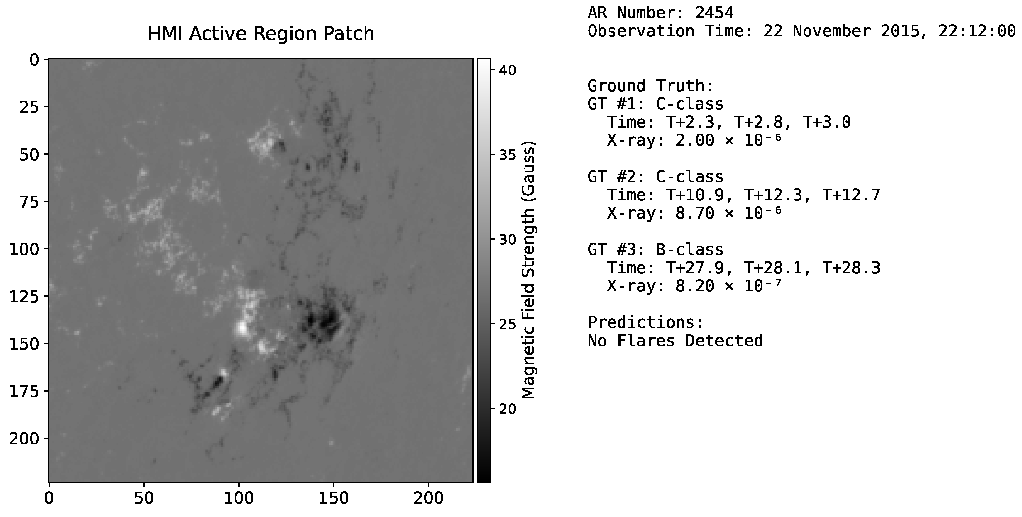
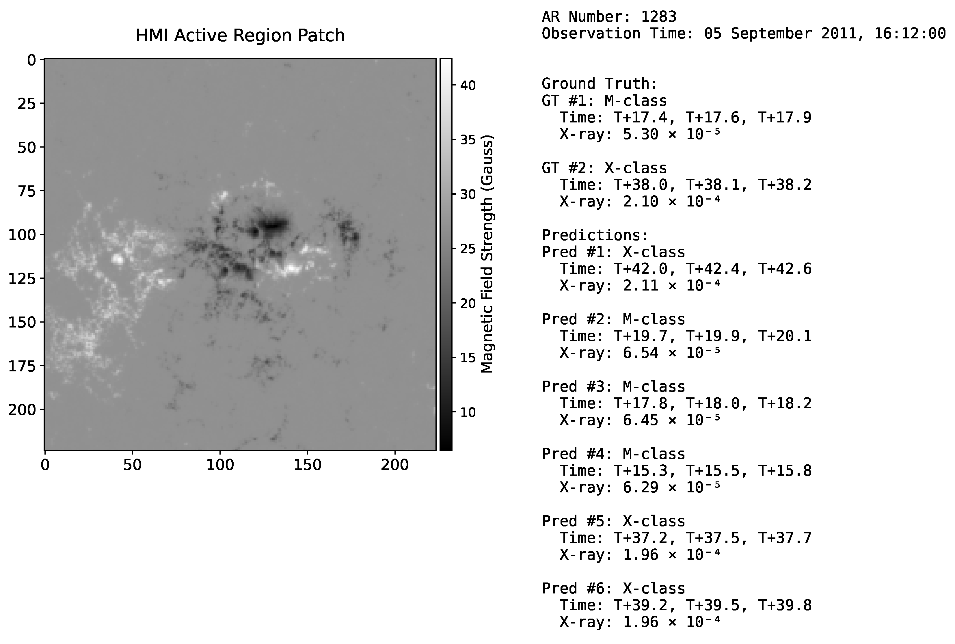
4.1. Inference Pipeline and Evaluation Matching

Obtaining and evaluating predictions from a trained FSPT model involves a dedicated inference pipeline. Given an input HMI magnetogram, the model (operating in evaluation mode) performs a forward pass, generating raw outputs (confidence scores, normalized time offsets, and base-10 logarithm of density with normalization) for all N object queries. These outputs are de-normalized to their physical scales (hours, W/m²).

Similar to typical object detection pipelines like DETR, candidate predictions are then obtained by filtering the raw outputs based on a confidence threshold (e.g., >0.05). However, the subsequent step—matching these candidates to ground-truth flares for performance evaluation—fundamentally differs from that of standard procedures.

To further evaluate the model’s practical applicability and provide concrete examples of its predictive performance, we present sample prediction cases. Figure 2, Figure 3 and Figure 4 showcase selected prediction instances, visually comparing the model’s outputs—including the X-ray intensity and time offset predictions—against the ground-truth solar flare events. These examples help illustrate how the model performs in different scenarios. For instance, Figure 2 (Sample A: AR 1283; 12 November 2012) displays an instance of a correct prediction; the input HMI active-region patch is shown on the left, and in the right panel, the single ground-truth flare is successfully identified by the model, resulting in one True Positive (TP). In contrast, Figure 3 (Sample B: AR 2454; 12 November 2015) demonstrates a case of missed detections. Here, three ground-truth flares occurred, but the model did not produce any corresponding predictions, leading to three False Negatives (FNs). Figure 4 (Sample C: AR 1283; 5 September 2011) exemplifies a scenario with two ground-truth flares, where the model generated six predictions. Two of these were correctly matched to the ground-truth flares (two TPs), while the remaining four were False Positives (FPs), indicating instances of over-prediction or false alarms. These visual case studies offer insights into the model’s behavior and the nature of True Positives, False Positives, and False Negatives that are quantified in our subsequent evaluation.

This evaluation matching, distinct from the Hungarian algorithm used during training (Section 3.2), serves solely to determine the True Positives (TPs), False Positives (FPs), and False Negatives (FNs) for metric calculation. It employs a confidence-driven greedy approach. Crucially, unlike standard object detection evaluation (e.g., COCO metrics relevant for DETR, which rely on Intersection-over-Union (IoU) thresholds between bounding boxes), FSPT’s evaluation matching uses domain-specific criteria based on the predicted flare characteristics. A candidate prediction is matched to an available ground-truth flare (one-to-one) only if it satisfies strict the criteria for both temporal proximity (all three predicted time offsets—start, peak, and end—must be within 6.0 h of their corresponding ground-truth times) and intensity similarity (the ratio of predicted to ground-truth peak intensity must be between $1/3$ and 3).

The resulting TP, FP, and FN counts across the evaluation dataset form the basis for calculating the performance metrics discussed next (Section 4.2).

4.2. Evaluation Metrics

Evaluating the performance of a set-prediction model like FSPT requires metrics that can assess the quality of the predicted set against the ground-truth set of flares. Traditional metrics used for binary classification tasks in solar flare forecasting are not directly applicable. Therefore, we adopt metrics commonly used in object detection and adapted for our specific task: F1-score and Average Precision (AP).

Metrics such as precision, recall, and F1-score are calculated based on the counts of True Positives (TPs), False Positives (FPs), and False Negatives (FNs) derived from the evaluation matching process described in Section 4.1. For a given confidence threshold $\tau$, TP($\tau$) is defined as the number of predictions with confidence $\ge \tau$ that are successfully matched to a ground-truth flare; FP($\tau$) is the number of predictions with confidence $\ge \tau$ that remain unmatched; and FN($\tau$) corresponds to the number of ground-truth flares not matched by any prediction with confidence $\ge \tau$. Precision and recall at threshold $\tau$ are then defined as

$$\mathrm{Precision}\left(\tau \right)={\displaystyle \frac{\mathrm{TP}\left(\tau \right)}{\mathrm{TP}\left(\tau \right)+\mathrm{FP}\left(\tau \right)}}$$

$$\mathrm{Recall}\left(\tau \right)={\displaystyle \frac{\mathrm{TP}\left(\tau \right)}{\mathrm{TP}\left(\tau \right)+\mathrm{FN}\left(\tau \right)}}$$

The F1-score, the harmonic mean of precision and recall, is

$$\mathrm{F}1\left(\tau \right)=2\times {\displaystyle \frac{\mathrm{Precision}\left(\tau \right)\times \mathrm{Recall}\left(\tau \right)}{\mathrm{Precision}\left(\tau \right)+\mathrm{Recall}\left(\tau \right)}}$$

In our evaluation procedure, we calculate these metrics at specific predefined confidence thresholds (e.g., [0.5, 0.7]), providing insights into performance at different operating points.

While F1-scores at fixed thresholds are informative, Average Precision (AP) provides a single-figure summary of the model’s performance across all possible confidence thresholds. It is calculated as the area under the precision–recall curve. The curve is generated by considering all predictions with confidence above a minimum threshold (0.05), sorting them by confidence, and plotting precision against recall as the confidence threshold is varied implicitly from high to low. The calculation follows standard methodologies, often similar to the COCO evaluation protocol [30], but with a crucial distinction regarding the definition of a True Positive. In standard object detection, a TP is typically determined by the Intersection over Union (IoU) between a predicted bounding box and a ground-truth box exceeding a certain threshold. For FSPT, as detailed in Section 4.1, a TP is determined by satisfying our custom-defined, domain-specific criteria based on temporal proximity (start, peak, and end time errors all below a threshold) and peak X-ray intensity similarity (ratio within a factor). This use of physically meaningful matching criteria, rather than spatial IoU, is fundamental to evaluating the set-prediction performance for this specific scientific application.

Furthermore, metrics widely used in traditional solar flare forecasting, like the True Skill Statistic (TSS), Heidke Skill Score (HSS), and Gilbert Skill Score (GSS), are generally inapplicable here. These metrics, often evaluated based on a $2\times 2$ contingency table [31], fundamentally rely on the concept of True Negatives (TNs), which represent correctly predicted negative instances (i.e., correctly forecasting no event). For a set-prediction model like FSPT, which outputs a variable-sized set of potential events rather than a single binary prediction for the forecast window, the concept of a TN is ill-defined. Unmatched queries with low confidence represent the absence of a detected object, not a global prediction of inactivity, making it impossible to derive the TN count required by these skill scores [31]. Consequently, skill scores heavily dependent on TN are unsuitable for evaluating set-prediction models in this context.

4.3. Evaluation Results

The quantitative performance of the FSPT model on the test set, evaluated using the metrics defined in Section 4.2 and the matching criteria specified in Section 4.1, is summarized below.

Table 3. Performance metrics of FSPT on the test set at different confidence thresholds.

Confidence Threshold ($\mathit{\tau }$)	Precision ($\mathit{\tau }$)	Recall ($\mathit{\tau }$)	F1-Score ($\mathit{\tau }$)
0.1	0.2209	0.9495	0.3584
0.3	0.2817	0.9299	0.4324
0.5	0.4609	0.7719	0.5772
0.7	0.8258	0.2474	0.3808
0.9	0.0000	0.0000	0.0000

presents the precision, recall, and F1-score at various confidence thresholds, illustrating the trade-offs at different operating points.

In addition to the threshold-specific metrics, the overall performance across all confidence levels was captured by the Average Precision (AP). The calculated AP for FSPT on the test set was 0.6565. Furthermore, the model’s accuracy in predicting the temporal evolution was assessed by the average Mean Absolute Error (MAE) across the predicted start, peak, and end time offsets and was found to be 2.2638 h.

The relationship between precision and recall across different confidence thresholds is visualized by the precision-recall curve shown in Figure 5. This curve illustrates the trade-off inherent in the model: achieving higher precision (fewer false positives among predicted flares) typically comes at the cost of lower recall (missing more true flares), and vice versa. The area under this curve represents the AP value reported above (0.6565), summarizing the overall performance across all thresholds.

These results warrant further discussion. The obtained AP of 0.6565 suggests that the model possesses a reasonable capability to rank correct flare predictions higher than incorrect ones across various confidence levels. While there is considerable room for improvement, this score provides initial validation for the feasibility of FSPT as a set-prediction model for this task.

However, it is important to contextualize this AP score and our F1-scores. While acknowledging that direct comparison is challenging due to vastly different task formulations and even F1-score definitions, it is true that some previous works focusing on binary flare forecasting have reported F1-scores in the 0.8–0.9 range for predicting flare occurrence [11,12,14,15,17]. Our model’s peak F1-score of 0.5772 (at a 0.5 confidence threshold), evaluated under the more demanding criteria of set prediction with specific characterization, admittedly does not represent a performance increase in the traditional, simpler classification sense. Direct comparison with metrics from traditional classification-based flare prediction models is generally inappropriate due to the fundamental difference in the tasks evaluated.

FSPT, however, predicts a set of flares, each with specific start times, peak times, end times, and intensities.

This capability for direct set prediction is fundamentally enabled by its architecture, which is inspired by the DETR framework [19]. Within FSPT, the transformer encoder–decoder is not merely a supplementary module but the core engine that processes object queries into a variable-sized set of predictions. These processed queries are then passed to relatively simple feed-forward networks (MLPs) acting as prediction heads; their "customization" lies in tailoring the output dimensions and activation functions to directly regress the specific characteristics of each flare event, rather than in complex, novel head architectures. The primary feature extraction and relational reasoning are performed by the ResNet backbone and the transformer, respectively. Given the integral nature of the transformer to this set-prediction paradigm—where its removal would dismantle the model’s core operational principles—the reported performance reflects the efficacy of this holistic architectural approach. This contrasts with assessing isolated contributions of such foundational components through traditional ablation studies, which are less straightforward in this context.

Our metrics (AP and F1@threshold) evaluate the model’s ability to correctly identify the number of flares and accurately predict the characteristics of each individual flare in the set.

Nevertheless, our research remains significant because it pioneers a more informative and challenging prediction paradigm. This difference in evaluation depth is particularly evident when considering temporal and intensity predictions. Traditional models are typically evaluated on whether any flare above a certain class threshold occurs within a broad window. In contrast, FSPT predicts specific start, peak, and end times for each individual flare. Our evaluation matching (Section 4.1) enforces a strict temporal constraint: a prediction is only considered a match if the predicted start, peak, and end times are all within 6.0 h of the true times.

Exploring the sensitivity of model performance to variations in this 6.0-h temporal tolerance could be a subject for future investigation, although it would require considerable computational resources for retraining and re-evaluation with each threshold.

This requirement for simultaneous temporal alignment across all three points represents a significantly higher bar and temporal resolution compared to the coarse window-based assessment of classification models. Similarly, for X-ray intensity, classification models predict broad logarithmic categories (A, B, C, M, and X), whereas FSPT predicts a specific peak intensity value, and our evaluation requires this prediction to be within a factor of 3 (i.e., between $1/3$ and 3 times the true value) of the ground-truth intensity. This reflects a finer granularity in evaluating the predicted physical properties.

This “factor of 3” criterion, which can be expressed as the ratio $I_{\mathrm{pred}}/I_{\mathrm{gt}}\in [1/3,3]$, was specifically chosen to effectively match intensities on a logarithmic scale. It is equivalent to requiring the absolute difference between their base-10 logarithms to be less than or equal to ${log}_{10}\left(3\right)\approx 0.477$. This approach is crucial for appropriately handling the wide dynamic range of flare intensities and their characteristic scale-free statistical distribution, which is a hallmark of phenomena like solar flares that exhibit Self-Organized Criticality (SOC).

Furthermore, it is important to acknowledge that the FSPT model’s DETR-based architecture relies on a Hungarian matching algorithm during evaluation, which holistically aligns the entire predicted set of parameters against the ground truth for each potential flare. While assessing the prediction accuracy for each output variable (e.g., start time or peak intensity) independently could offer further insights, cleanly disentangling such individual performances from this integrated matching framework is not straightforward, as a successful match is determined by the collective accuracy of all predicted characteristics meeting their respective criteria simultaneously. The stringency of these combined matching criteria should therefore be considered when interpreting the resulting AP scores, potentially explaining why they may appear modest compared to classification metrics evaluated under less stringent conditions.

The value of FSPT lies in its potential to provide these detailed, actionable predictions for multiple events, a capability largely absent in traditional approaches, rather than solely optimizing a single metric for a binary outcome.

Examining the threshold-specific metrics in Table 3 further reveals the precision–recall trade-off: lower thresholds (e.g., $0.1$ and $0.3$) yielded high recall (>0.9) at the cost of low precision, suggesting that the model identified most true flares but also generated many false positives. Conversely, a high threshold like 0.7 achieved high precision (0.8258) but low recall (0.2474), indicating that high-confidence predictions were likely correct but many true flares were missed. The balanced F1-score peaked around the 0.5 threshold (0.5772). The zero performance at the 0.9 threshold likely stemmed from a combination of factors, including the inherent imbalance between the number of object queries (N = 100) and the typically small number of ground-truth flares per sample, making it exceptionally challenging for the model to assign extremely high confidence while simultaneously meeting the strict matching criteria. This highlights the difficulty of achieving both high confidence and high regression accuracy concurrently in this sparse set-prediction task.

Despite the strict matching criteria, the average time MAE of 2.26 h reflects a reasonable accuracy in predicting temporal characteristics. Compared to the 6.0-h tolerance used for matching, this average error indicates that the model often predicted flare timings well within the acceptable range, representing a significant step toward providing temporally specific predictions, although further refinement is needed for operational precision, particularly for rapid events.

It is crucial to recognize the enhanced informational value offered by the set-prediction approach. Unlike classification models that yield only probabilities for broad categories, FSPT aims to predict the number, timing, and intensity of individual flares. This richer output, despite current accuracy limitations needing further development, offers the potential for more nuanced risk assessment and targeted mitigation strategies, demonstrating the promise of this forecasting paradigm.

5. Conclusions and Future Work

Traditional machine learning approaches to solar flare prediction have predominantly framed the problem as a classification task, predicting the likelihood of broadly categorized events within fixed time windows. While successful in improving forecast skill scores like TSS, this paradigm inherently limits the richness of the prediction, failing to provide details on the number, timing, and intensity of individual flare events. In this paper, we propose and demonstrate a fundamental paradigm shift by reformulating solar flare prediction as a set-prediction problem. This approach aims to directly predict a variable-sized set of flare events, each characterized by specific properties. The core contribution of this work lies in the proposal of this new framework that enables forecasts that are significantly more informative and physically relevant than those of prior approaches, as it is capable of predicting the multiplicity of flares along with their individual start, peak, and end times, as well as their peak soft X-ray intensities.

To realize this paradigm, we introduce FSPT, a transformer-based model inspired by the DETR architecture from object detection. We detail the necessary adaptations, including the modifications to the backbone’s input layer, the design of prediction heads for temporal offsets and intensity, and the implementation of a set-based loss function incorporating the focal loss and L1 regression terms. Crucial supporting work involves developing a novel dataset-labeling scheme to generate the required set-based targets from observational data and implementing a careful dataset-splitting strategy using AR grouping and simulated annealing to mitigate data leakage and ensure distributional balance. Our evaluation, utilizing metrics appropriate for set prediction (AP and F1-score based on stringent temporal and intensity matching criteria), demonstrates the viability of the FSPT model. The model achieves promising results (e.g., F1-score of 0.5772 at 0.5 confidence threshold, and AP of 0.6565), demonstrating its capability to predict the detailed characteristics of individual flares with reasonable accuracy (time MAE: 2.2638 h). Importantly, we establish an evaluation methodology tailored to this task, highlighting the inadequacy of traditional TN-dependent skill scores (TSS, HSS, and GSS) for set-prediction models and clarifying why direct comparison with classification-based model metrics is inappropriate due to the fundamental difference in the prediction task.

Despite these promising results, it is appropriate to view FSPT as a preliminary exploration—a rough start—within this new paradigm. Its current limitations also highlight avenues for future research. The achieved F1/AP scores indicate scope for improvement in predictive accuracy, and the average time MAE (2.26 h), while reasonable within the 6-h matching tolerance, suggests that achieving high temporal precision remains challenging, especially for fast-evolving events. Furthermore, the current model lacks spatial location prediction. Nonetheless, this work successfully demonstrates the potential of the set-prediction paradigm for providing richer, more detailed, and actionable solar flare forecasts.

This foundational work opens several promising avenues for future research, which can be broadly categorized. First, efforts should focus on enhancing the model’s predictive performance. This includes expanding the dataset to encompass longer time periods and diverse solar cycles to improve generalization and robustness, particularly addressing the effective sample size limitations discussed in Section 2. Exploring the scaling of both inputs and models, such as migrating to higher-resolution, multi-channel full-disk magnetograms alongside correspondingly larger architectures, could yield richer predictive signals, albeit at increased computational cost. Furthermore, leveraging temporal dynamics via sequences of magnetograms (i.e., video data) offers a promising direction for explicitly capturing evolutionary patterns, potentially boosting predictive performance. A significant further ambition involves incorporating spatial information to achieve comprehensive spatio-temporal forecasting, predicting not only when and how strong a flare will be but also where it will occur. However, it is precisely when aiming for such detailed predictions that we must confront the fundamental nature of solar flares as Self-Organized Criticality (SOC) phenomena. The inherent characteristic of SOC systems, particularly the scale-free distribution of event sizes where minor disturbances can potentially trigger events of any magnitude, raises profound questions about the ultimate feasibility of deterministic, high-precision spatio-temporal forecasting. While the quest to predict all these features remains an open scientific challenge, the pursuit itself is invaluable. Incremental advancements in predictive scope, probabilistic accuracy, or lead times offer significant practical benefits for space-weather mitigation, and critically, these research endeavors deepen our understanding of the underlying physical mechanisms, regardless of whether perfect prediction is ultimately attainable. Future iterations should therefore explore methodologies for integrating spatial coordinates and full-disk magnetograms while concurrently investigating the theoretical limits of predictability imposed by the SOC nature of flares.

Second, future work should aim to increase the model’s forecasting capabilities. A significant next step is incorporating spatial information; future iterations should aim to utilize full-disk magnetograms and integrate spatial coordinates into the labels for comprehensive spatio-temporal forecasting, predicting not only when and how strong a flare will be but also where it will occur.

Finally, bridging the gap toward operational utility is a key goal. This involves developing and potentially deploying a real-time version of FSPT, perhaps accessible via a web interface, to provide timely and actionable forecasts for space-weather stakeholders.

By focusing on these future directions in performance, capability, and utility, we can better realize the full potential of the set-prediction paradigm for advancing operational solar flare forecasting capabilities, with the expectation of significant metric improvements accompanying these developments.

References

1. Priest, E.R.; Forbes, T.G. Magnetic Reconnection. Astron. Astrophys. Rev. 2002, 10, 313–377. [Google Scholar] [CrossRef]
2. Bornmann, P.L.; Shaw, D. Flare Rates and the McIntosh Active-Region Classifications. Sol. Phys. 1994, 150, 127–146. [Google Scholar] [CrossRef]
3. Wheatland, M.S. A Bayesian Approach to Solar Flare Prediction. Astrophys. J. 2004, 609, 1134–1139. [Google Scholar] [CrossRef]
4. Bloomfield, D.S.; Higgins, P.A.; McAteer, R.T.J.; Gallagher, P.T. Toward Reliable Benchmarking of Solar Flare Forecasting Methods. Astrophys. J. Lett. 2012, 747, L41. [Google Scholar] [CrossRef]
5. Bobra, M.G.; Couvidat, S. Solar Flare Prediction Using SDO/HMI Vector Magnetic Field Data with a Machine-learning Algorithm. Astrophys. J. 2015, 798, 135. [Google Scholar] [CrossRef]
6. Liu, C.; Deng, N.; Wang, J.T.L.; Wang, H. Predicting Solar Flares Using SDO/HMI Vector Magnetic Data Products and a Random Forest Algorithm. Astrophys. J. 2017, 843, 104. [Google Scholar] [CrossRef]
7. Florios, K.; Kontogiannis, I.; Park, S.H.; Guerra, J.A.; Benvenuto, F.; Bloomfield, D.S.; Georgoulis, M.K. Forecasting Solar Flares Using Magnetogram-based Predictors and Machine Learning. Sol. Phys. 2018, 293, 28. [Google Scholar] [CrossRef]
8. Nishizuka, N.; Sugiura, K.; Kubo, Y.; Den, M.; Watari, S.; Ishii, M. Solar Flare Prediction Model with Three Machine-learning Algorithms using Ultraviolet Brightening and Vector Magnetograms. Astrophys. J. 2017, 835, 156. [Google Scholar] [CrossRef]
9. Nishizuka, N.; Sugiura, K.; Kubo, Y.; Den, M.; Ishii, M. Deep Flare Net (DeFN) for Stokes Profiles of Solar Flares. Astrophys. J. 2018, 858, 118. [Google Scholar] [CrossRef]
10. Zheng, J.; Xu, J.; Wang, W.; Zhang, H. Solar Flare Prediction Using Hybrid Deep Neural Networks. Sol. Phys. 2019, 294, 11. [Google Scholar] [CrossRef]
11. Huang, X.; Wang, H.; Xu, L.; Liu, J.; Li, R.; Dai, X. Deep Learning Based Solar Flare Forecasting Model. I. Results for Line-of-sight Magnetograms. Astrophys. J. 2018, 856, 7. [Google Scholar] [CrossRef]
12. Park, E.; Moon, Y.J.; Shin, S.; Yi, K.; Lim, D.; Lee, H.; Shin, G. Application of the Deep Convolutional Neural Network to the Forecast of Solar Flare Occurrence Using Full-disk Solar Magnetograms. Astrophys. J. 2018, 869, 91. [Google Scholar] [CrossRef]
13. Zhang, H.; Li, Q.; Yang, Y.; Jing, J.; Wang, J.T.L.; Wang, H.; Shang, Z. Solar flare index prediction using SDO/HMI vector magnetic data products with statistical and machine-learning methods. Astrophys. J. Suppl. Ser. 2022, 263, 28. [Google Scholar] [CrossRef]
14. Li, X.; Zheng, Y.; Wang, X.; Wang, L. Predicting Solar Flares Using a Novel Deep Convolutional Neural Network. Astrophys. J. 2020, 891, 10. [Google Scholar] [CrossRef]
15. Chen, Y.; Manchester, W.B.; Hero, A.O.; Toth, G.; DuFumier, B.; Zhou, T.; Wang, X.; Zhu, H.; Sun, Z.; Gombosi, T.I. Identifying Solar Flare Precursors Using Time Series of SDO/HMI Images and SHARP Parameters. Space Weather 2019, 17, 1404–1426. [Google Scholar] [CrossRef]
16. Wang, X.; Chen, Y.; Toth, G.; Manchester, W.B.; Gombosi, T.I.; Hero, A.O.; Jiao, Z.; Sun, H.; Jin, M.; Liu, Y. Predicting Solar Flares with Machine Learning: Investigating Solar Cycle Dependence. Astrophys. J. 2020, 895, 3. [Google Scholar] [CrossRef]
17. Pandey, C.; Adeyeha, T.; Hong, J.; Angryk, R.A.; Aydin, B. Advancing Solar Flare Prediction Using Deep Learning with Active Region Patches. In Proceedings of the Machine Learning and Knowledge Discovery in Databases. Applied Data Science Track (ECML PKDD 2024), Vilnius, Lithuania, 9–13 September 2024; Springer: Berlin/Heidelberg, Germany, 2024; pp. 50–65. [Google Scholar] [CrossRef]
18. Qin, G.; Zhang, M.; Rassoul, H.K. Transport of Solar Energetic Particles in Interplanetary Space. J. Geophys. Res. Space Phys. 2009, 114, A09104. [Google Scholar] [CrossRef]
19. Carion, N.; Massa, F.; Synnaeve, G.; Usunier, N.; Kirillov, A.; Zagoruyko, S. End-to-end object detection with transformers. In Proceedings of the Computer Vision—ECCV 2020: 16th European Conference, Glasgow, UK, 23–28 August 2020; Springer: Berlin/Heidelberg, Germany, 2020; pp. 213–229. [Google Scholar] [CrossRef]
20. Boucheron, L.E.; Vincent, T.; Grajeda, J.A.; Wuest, E. Solar active region magnetogram image dataset for studies of space weather. Sci. Data 2023, 10, 825. [Google Scholar] [CrossRef]
21. Schou, J.; Scherrer, P.H.; Bush, R.I.; Wachter, R.; Couvidat, S.; Rabello-Soares, M.C.; Bogart, R.S.; Hoeksema, J.T.; Liu, Y.; Duvall, T.L.; et al. Design and Ground Calibration of the Helioseismic and Magnetic Imager (HMI) Instrument on the Solar Dynamics Observatory (SDO). Sol. Phys. 2012, 275, 229–259. [Google Scholar] [CrossRef]
22. Bobra, M.G.; Sun, X.; Hoeksema, J.T.; Turmon, M.; Liu, Y.; Hayashi, K.; Barnes, G.; Leka, K.D. The Helioseismic and Magnetic Imager (HMI) Vector Magnetic Field Pipeline: SHARPs–Space-Weather HMI Active Region Patches. Sol. Phys. 2014, 289, 3549–3578. [Google Scholar] [CrossRef]
23. He, K.; Zhang, X.; Ren, S.; Sun, J. Deep Residual Learning for Image Recognition. In Proceedings of the 2016 IEEE Conference on Computer Vision and Pattern Recognition (CVPR), Las Vegas, NV, USA, 27–30 June 2016; pp. 770–778. [Google Scholar]
24. Vaswani, A.; Shazeer, N.; Parmar, N.; Uszkoreit, J.; Jones, L.; Gomez, A.N.; Kaiser, Ł.; Polosukhin, I. Attention is all you need. Advances in neural information processing systems. arXiv 2017, arXiv:1706.03762. [Google Scholar] [CrossRef]
25. Kuhn, H.W. The Hungarian method for the assignment problem. Nav. Res. Logist. Q. 1955, 2, 83–97. [Google Scholar] [CrossRef]
26. Lin, T.Y.; Goyal, P.; Girshick, R.; He, K.; Dollár, P. Focal Loss for Dense Object Detection. In Proceedings of the 2017 IEEE International Conference on Computer Vision (ICCV), Venice, Italy, 22–29 October 2017; pp. 2999–3007. [Google Scholar]
27. Loshchilov, I.; Hutter, F. Decoupled weight decay regularization. arXiv 2017, arXiv:1711.05101. [Google Scholar] [CrossRef]
28. Smith, L.N.; Topin, N. Super-convergence: Very fast training of neural networks using large learning rates. In Artificial Intelligence and Machine Learning for Multi-Domain Operations Applications; SPIE: Bellingham, WA, USA, 2019; Volume 11006, pp. 369–386. [Google Scholar]
29. Deng, J.; Dong, W.; Socher, R.; Li, L.J.; Li, K.; Li, F.F. ImageNet: A large-scale hierarchical image database. In Proceedings of the 2009 IEEE Conference on Computer Vision and Pattern Recognition, Miami, FL, USA, 20–26 June 2009; pp. 248–255. [Google Scholar]
30. Lin, T.Y.; Maire, M.; Belongie, S.; Hays, J.; Perona, P.; Ramanan, D.; Dollár, P.; Zitnick, C.L. Microsoft COCO: Common Objects in Context. In Proceedings of the Computer Vision–ECCV 2014, Zurich, Switzerland, 6–12 September 2014; Springer: Berlin/Heidelberg, Germany, 2014; pp. 740–755. [Google Scholar]
31. Barnes, G.; Leka, K.D.; Schrijver, C.J.; Colak, T.; Qahwaji, R.; Ashamari, O.W.; Yuan, Y.; Zhang, J.; McAteer, R.T.J.; Bloomfield, D.S.; et al. A Comparison of Flare Forecasting Methods. I. Results from the “All-Clear” Workshop. Astrophys. J. 2016, 829, 89. [Google Scholar] [CrossRef]
Figure 1. Overall architecture of the FSPT model. An input HMI magnetogram is processed by a ResNet-18 backbone, followed by a transformer encoder–decoder. Finally, prediction heads (MLPs) generate the set of flare predictions, including confidence scores, time offsets, and peak X-ray intensity for each potential flare represented by an object query.
Universe 11 00174 g001
Figure 2. Input for Sample A (AR 1283; 12 November 2012 16:12:00) and the corresponding model inference result, illustrating a True Positive (TP) case. The left panel shows the input HMI active-region patch, and the right panel compares the ground-truth flare with the model’s prediction.
Universe 11 00174 g002
Figure 3. Input for Sample B (AR 2454; 12 November 2015 22:12:00) and the corresponding model inference result, illustrating a case of three False Negatives (FNs) where ground-truth flares were missed.
Universe 11 00174 g003
Figure 4. Input for Sample C (AR 1283; 5 September 2011 16:12:00) and the corresponding model inference result, illustrating a case with two True Positives (TPs) and four False Positives (FPs).
Universe 11 00174 g004
Figure 5. Precision–recall curve for the FlareTR model evaluated on the test set. The curve shows the trade-off between precision and recall for different confidence thresholds. The area under this curve corresponds to the Average Precision (AP) metric.
Universe 11 00174 g005