Abstract
Viewing high-redshift sources at near-opposite directions on the sky can ensure, using light-travel-time arguments, acausality between their emitted photons. One utility would be true random-number generation through sensing these via two independent telescopes that each flip a switch based on the latest-arrived colours; for example, to autonomously control a quantum-mechanical (QM) experiment. Although demonstrated with distant quasars, those were not fully acausal pairs, which are restricted when simultaneously viewed from the ground at any single observatory. In optical light, such faint sources also require a large telescope aperture to avoid sampling assumptions when imaged at fast camera framerates: unsensed intrinsic correlations between them or equivalently correlated noise may ruin the expectation of pure randomness. One such case that could spoil a QM test is considered. Based on that, the allowed geometries and instrumental limits are modelled for any two ground-based sites, and their data are simulated. For comparison, an analysis of photometry from the Gemini twin 8 m telescopes is presented using the archival data of well-separated bright stars obtained with the instruments ‘Alopeke (on Gemini North in Hawai’i) and Zorro (on Gemini-South in Chile) simultaneously in two bands (centred at and ) with 17 Hz framerate. No flux correlation is found; these results were used to calibrate an analytic model predicting where a search with a signal-to-noise over 50 at 50 Hz can be made using the same instrumentation. Finally, the software PDQ (Predict Different Quasars) is presented, which searches a large catalogue of known quasars, reporting those with a brightness and visibility suitable to verify acausal, uncorrelated photons at these limits.
1. Introduction
That quantum mechanics (QM) must be incomplete, allowing “spooky” outcomes requiring either super-luminal signals or hidden variables—essentially, unsensed influences on the outcome—was posited by Einstein, Podolsky, and Rosen [1]. Bell showed, however, that correlations in a QM experiment could allow for tests to obtain evidence against such hidden-variable theories [2]. Repeated Bell-theorem tests have since routinely found that QM is correct through tightly and simultaneously restricting the necessary conditions on measurements (e.g., [3] and references therein), including the influence of experimenter interaction: the so-called “freedom-of-choice” loophole. One route to this has been to set experimental parameters via photons from astronomical sources [4,5], requiring that interference in such settings is somehow orchestrated between distant sources and the Earth-based observer. Proof-of-concept tests using stars within the Milky Way were achieved [6] forcing any collusion in the outcome back hundreds of years. Additionally, the extension to quasars [7,8,9] pushed this to , combining high redshift z with large angular separation on the sky to increasingly place these outside each others’ light cone; where apart would be complete if both sources have [4]. Smaller separations could be compensated by higher source redshifts, although possibly at the cost of the objects being fainter. The motivation to reach this limit is to achieve independence from the settings triggered via those photons, which are unspoiled by communication. However, that is true only if no correlated errors are introduced via scattered photons from the sky, or otherwise via optical inefficiencies and detector electronics, which corrupt their unsychronized fluxes just prior to detection.
To outline the timescales and error limits that need to be met so that the flux of two quasars is truly acausal and measured as sufficiently uncorrelated, consider the one quasar-based Bell test undertaken so far by Rauch et al. [9]. This followed the methodology of Clauser [10], where an entangled pair of photons emitted from a central source are split between two optical arms and their polarizations are detected at receivers. While those entangled photons were in flight, a switching mechanism at each receiver (also co-located with a telescope) selected between two polarization measurements at pre-fixed relative angles, which were chosen to test the maximum potentially observable difference from QM. This switch was set using the colour of the most recently detected quasar photon: a dichroic splitting flux into two broad colour-bands that did not systematically favour either selection. Bright pairs were viewed separately via two 4 m class telescopes from Observatorio del Roque de los Muchachos on La Palma. One quasar pair was separated by on the sky, with and ; another pair was apart with and . Both quasar fluxes (in ) were brighter than the sky background () and a relative polarization measurement was retained only if both quasar photons arrived within microseconds while the entangled photons were in flight. Fair sampling was assumed; that is, thousands of individual trials were obtained non-continuously (achieving a duty cycle up to several seconds apart; the cadence ) during runs lasted 12 and 17 min and so each quasar-photon sample initiating a switch was considered independent, providing no information that could be exploited to predict the next outcome. This meant that at least one in four correlated switching photons were needed to spoil a Bell test, although possibly as little as 14% is enough [11]. Thw analysis showed that neither the colours of the two quasars nor the background noise hindering their detection (i.e., sky-line fluctuations) were correlated among all trials beyond such measurement-error margins.
Optical or near-infrared (NIR) photometry from any single observatory site hinders a QM-test experimental cadence fast enough to remove the fair-sampling assumption for quasars separated by more than where both have . That is due to the two switching telescopes being, at most, kilometers apart, where is in light travel time, i.e., ∼1 MHz rates. However, a typical quasar has a V-band AB-magnitude of about 20 [12] (roughly the same as the dark sky in ) and similar to 1 micron, which, even for an idealized unobstructed 8 m class telescope with perfect throughput (that splits light into two bandpasses), provides a fluence of less than 18 photons in 10 milliseconds under photometric skies at low elevation when operating at a reasonable observing limit of extinction. Despite a good vision of , this would be against a background of below 2 photons, providing an individual exposure signal-to-noise ratio (SNR) of over 10 for each quasar. A sampling cadence of would then be the fastest possible means of retaining a sufficient SNR against the sky background flux for the simultaneous two-band photometry of both quasars while reaching a colour-discrimination per sample of uncertainty, and this would work less well for realistic efficiencies. Finding brighter sources or choosing broader passbands could double the SNR, but this would still be four orders of magnitude slower than the telescope-to-telescope signalling rate. That is a problem because millisecond and longer-lasting oscillatory correlations might naturally arise due to the self-similar Kolmogorov scaling of wavefront aberrations, particularly at smaller telescope angular separations, without any ability to discriminate those against fluctuations due to the sources themselves. Adaptive optics (AO) may help, as such systems routinely sense these phase errors at kilohertz rates at wavelengths of near and utilize their index-of-refraction behaviour to manipulate them longward of or so into the NIR: these photons can be redirected with a fast-moving optic. This results in a sharpened image that may be diffraction-limited at , more readily improving photometry by a factor of 2 or so and leaving an uncorrected fraction at lower frequencies (e.g., [13]). However, even with this assistance, the practical sampling cadence is too slow to exclude all higher-frequency intrinsic correlations (or correlated noise) that can provide a prediction for the next experimental outcome, whether the quasar switching-photon sample of either band at each telescope falls inside the seeing disk or not.
Instead, telescopes situated at two well-separated sites could rule out such correlations, because then both high-angular separations of up to (and, therefore, known acausal sources) and fluctuations in seeing (and, therefore, source versus background flux per sample) need only be monitored at timescales closer to the Earth light-crossing time, roughly less than or at , to measure and exclude any influence (or temporally correlated errors) in their simultaneous photometry. Interestingly, no such case has been reported so far, and no monitoring campaign simultaneously viewing quasars outside each observatory’s horizon seems to have been undertaken, at any wavelength. For -rays and X-rays, and through to far-ultraviolet rays, this would require a specially designed spaceborne mission, which is not yet planned. This difficulty extends to the radio as, when on the ground, dish elevations must remain above the horizon regardless of Sun position. From Earth’s nightside, optical/NIR telescopes are restricted to separations below two airmasses, incurring about twice the zenith extinction and instrumental zeropoint error for each. Even so, non-AO corrected photometry to within 10% accuracy can still be achieved for these sources. Therefore, the goal of achieving simultaneous photometry at 10 Hz for 100 Hz-framerates of acausal quasar pairs with two independent telescopes may be within reach. What should they see?
The first step to answering that is to define a plausible correlated signal to look for, sufficient to spoil a Bell test, in order to characterize what might be detected within the observational noise—at best, within just the instrumental zeropoints—without assuming instrinsic randomness. Second is the characterization of instrumental limits, and demonstration of simultaneous high-framerate optical photometry from two widely separated sites, setting a benchmark. An active galactic nucleus (AGN) need not be the source. So, at least one useful dataset to probe is already available at Gemini, providing data on Maunakea in Hawaii ( N, W, 4213 m) and Cerro Pachon in Chile ( S, W, 2722 m); when each viewing a target near zenith, these data place those apart on the sky. These twin 8.1 m telescopes have operated as near-identical high-framerate (up to ) optical imagers for several years, as ‘Alopeke and Zorro, and their public archive contains some serendipitous, simultaneous observations of bright stars. Although such data do not constitute a QM experiment, they do provide a baseline when devising a future one: at over 10,600 km apart, no collusion is possible on timescales less than this distance divided by the speed of light or , which, in the restframe at , corresponds to .
The next section describes how the geometry of an experiment allowing for the simultaneous photometry of quasar pairs restricts their best relative SNR, if not due simply to correlated errors, AGN-physics can, at the short timescales relevant here, cause such an intrinsic signal to arise. Simulated observational data are generated. A method of sensing the correlation of flux differences will be described for conditions where point-source photometry has sufficient sampling and sensitivity to reach the zeropoints of two identical instruments within about 2% error. This is then extended to any two observation sites on Earth, including paired antipodal ones, and to fainter pairs appropriate for quasars. Following that, the available Gemini dataset is described: four observational pairs of bright stars with separations up to nearly in the sky and at a peak SNR consistent with the model, providing a calibration at sampling rate towards tests with quasars. Software is described that can finds these for follow-up tests at a framerate over . The discussion concludes with a short list of potential quasar-pairs and their upcoming best nights for observation via simultaneous Gemini photometry with ‘Alopeke/Zorro, which reaches the necessary photometric accuracy to prove suitability in a Bell test.
2. Methods of Finding Uncorrelated, Acausal Quasars
The approach taken here is to first define what correlation between two sources, whether intrinsic or from correlated noise, could be sufficient to spoil a QM test that employed those sources. Although it seems an improbable scenario, positing that some acausal source pair might be perfectly correlated establishes a falsifiable signal that can be looked for. This allows for a well-defined estimate of the SNR for the measurement of the differences in flux of all photons (both causal and acausal), and the production of simulated data. In this way, a model of the observational noise of the two sites can be used to find, via a catalog of known quasars, useful targets for which to initiate a search, despite expecting a null result.
2.1. A Plausible Correlated Quasar-Pair Signal to Look For
Maybe nature does provide a pair of quasars (call them sources A and B) that could not have communicated but always have perfectly correlated fluxes within two colour-filter passbands (labelled “blue” and “red”). If they exist, such a correlation can be found even if the long-term average relative A-B colour is constant. For example, imagine that the flux of A at a particular emission wavelength (within either the blue or red passband) is always anti-correlated with B in a sinusoidal function at constant frequency low enough to be detectable; say, one from seconds to minutes long. That is at least a plausible scenario, because the rotational periods of the AGN accretion disks or related structures in their jets are the source of the emission line and continuum photons under study here, and reverberation mapping has established the characteristic sizes of these in the order of light days across; they are known to be variable over these timescales and longer ones [14,15]. However, if these two disks have identical rotational periods, common physical scales of smaller substructures should also be correlated over shorter timescales of less than hours. This would be analogous to soundwaves behaving as a “siren” with a constant cycle or pitch but fluctuating intensity. All this is necessary for their detection and use (and as utilized in the experiment by Rauch et al.) while reliably reaching a minimum threshold flux in the blue and red passbands, providing correlated photons to predictably trigger the switches. Ideally, there will always be a reliable-frequency signal (oscillating between blue and red) of fixed amplitude.
When that frequency increases to the highest possible framerate at the switching telescopes, this amounts to the signals acting as an on/off “toggle switch”, which is either blue for the observer of A (designated hereafter as Alice) or red for the observer of B (Bob), or vice versa, at a constant frequency. This limit is illustrated schematically in Figure 1, where the filled black circles indicate the colour of a received sample of photons being at least one standard deviation from the mean (long-term average) colour of the received photons at both switching-station detectors. It will become clear why this particular limit was chosen. However, in this scenario, it is obvious that neither Alice nor Bob need know what colour photons the other received, because when they observe one state (sample 1 is blue), they are confident to two standard deviations of their combined noise sources that the opposite is currently the case for the other (red), and, furthermore, that sample 3 will return to the same state (blue, while the other is red again). The longer-term, lower-frequency limit for the detectable siren-like signal (shown for a period of 16 samples) is indicated by a smooth curve; this lower frequency is comparable (for 100 Hz sampling) to the outer limit of the clock precision of either receiving telescope.
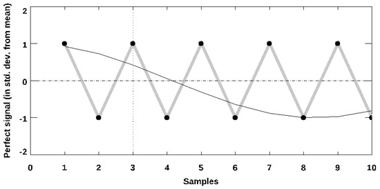
Figure 1.
A clear signal between two sources, A and B: a steady sinusoidal “siren” with a half-cycle of eight samples spanning two full standard-deviations of each receivers’ noise. Minimized to the fastest attainable framerate, this is a perfect “toggle switch” (filled circles, grey line segments).
2.2. Simulated Data with Correlated Signals and Gaussian Noise
Simulated data were generated for the A-B colour signal of Section 2.1, which are clearly exploitable to predict future settings, but degraded in such a way that they are only just sufficient at the receiver/switching stations to spoil a QM test. Figure 2 shows what would be observed if the signal as described in Figure 1 was mixed with white noise; that is, there is no correlation at all between the two sources. The IDL function RANDOMU was used for pseudo-random number generation. The intermediate case (shown in the top panel) occurs often enough to make the observers’ prediction of the next sample incorrect 25% of the time. To put this another way, Alice is still certain to receive a blue photon when Bob receives a red photon, on average, three out of four times, and similarly they reliably predict each other’s results. They need not know whether this is due to the intrinsic signal or correlated noise at detection. However, noise at the switching telescopes due to local sky conditions, detector noise, etc., if uncorrelated, must work randomly against the accuracy of the colour measurements at either station. Therefore, all noise at the telescopes is assumed, collectively, to be Gaussian, simulated using RANDOMN. The effects of adding one standard deviation of observational noise at each station are illustrated in the bottom two panels of Figure 2. It is notable that these two cases look very similar, but it will be seen that they are distinguishable.
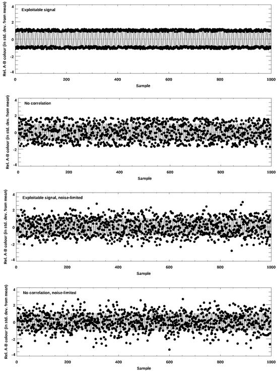
Figure 2.
Potential minimally “exploitable” A-B colour signal persisting for 1000 samples (top panel) and spanning the necessary one standard deviation from the median (shaded grey); a thin black curve indicates a perfect sinusoid or an equivalent distribution of pure white noise (second-to-top panel). The simulated observational sequences are as follows: just sufficient Gaussian noise to void its utility for exploitation in a QM test, or (bottom panel) no signal at all with the same amount of noise.
If the exploitable minimally correlated case does occur, it is important to note that this need not be detected in each individual difference; the underlying correlation is relative to the added and statistical noise. However, the correlation must persist for at least as long as an observation and have a frequency comparable to the sampling period. That is because the distribution of these A-B colours is measurably distinct, as illustrated in Figure 3. The top two panels are the distributions generated from the sequences shown in the top two panels of Figure 2. The grey-shaded band is the same one-standard-deviation range over which the colours must deviate in order to minimally detect the correlation. Notice that, in the perfect case of a toggle-switch, every sample at each receiver/switching station would be either blue (one std. dev. up from the mean) or red (one std. dev. down) exactly 50% of the time, even if not sequentially. In the top left-hand panel, it can be seen that this exploitable-signal case (thick black histogram) is no longer perfect, but shares the same attributes of the simple sinusoid (thin black curve). When degraded to one standard deviation of noise at each observing station, it now offers only a 50:50 prediction of the next outcome (losing its utility to spoil an experiment), but is noticeably not Guassian in distribution. On the contrary, for the cases with no underlying correlation, which are shown in the right-hand panels, the distribution of the detected colours is clearly Gaussian.
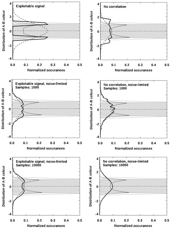
Figure 3.
Distributions of simulated samples, corresponding to the cases in Figure 2 as thick black curves. The top panels are for 1000 samples without observational noise, either assuming there is an exploitable signal (upper-left panel) or only white-noise, i.e., with no detectable correlation (upper-right panel); the case of a pure sinusoid is indicated as a thin black curve, and the ideal “toggle switch” is shown in thin light grey; a span of two standard deviations is shaded in grey. Below these top panels are those same cases, limited by observational noise, either for 1000 samples (middle panels) or 10,000 samples (bottom panels). Notice that a signal that just sufficient to exploit in defeating a QM experiment would remain discernibly different from an associated Gaussian-noise distribution, as indicated in each panel by a dashed-grey curve; even so, these have the same added observational noise.
Another way of establishing that there is no exploitable information is the auto-correlation of the signal shown in Figure 4, obtained by shifting each sample B sequence relative to the A sequence incrementally sample-by-sample and finding the colour difference. If some particular offset in time between the two signals does increase the correlation, this would cause a change relative to the mean colour difference. In this case, there is none, as expected. Note that the absolute difference in colours (in units of std. dev. from the mean) is always greater than 0.75 within a margin of about 0.02 (2% error); this corresponds to a correlation under 0.50 (again, imperfect by the same error margin), equivalent to even odds of predicting the colour in any sample for either A or B. To help compare, a vertical dotted line indicates the first eight samples, with the sinusoidal curve of Section 2.1 being overplotted. The upward-pointing and downward-pointing triangles are the first high and last low results within that span. This illustrates that, despite the seeming correlation (these do appear to agree with the trend), these samples are random; a signal is not present. It is helpful to look back to Figure 2; notice that this result corresponds to the lower right panel, with a Gaussian distribution. The case in the lower left panel is a distinctly bimodal distribution, with sufficient noise to render its signal insufficient to defeat a Bell test.
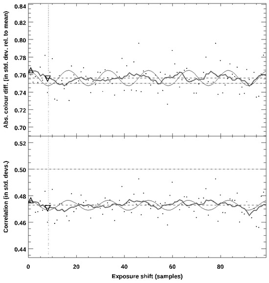
Figure 4.
Auto-correlation of a 1000-sample simulated sequence, limited by noise; each point is the result of taking the difference after shifting by that number of samples. No correlation is detectable.
2.3. Incorporating Site Conditions into a Model of Measureable Signal-to-Noise Ratio
Whatever the observable A-B colour signal of two point sources at a high angular separation, and acausal, where unseparated, it must be in the best possible conditions, with both telescopes pointed at a single source. In that case, the probability P of those two telescopes sensing a perfect correlation among the emitted photons (without noise) reaches exact unity,
where is the colour (in magnitude) per sample of the source: the perfectly correlated difference in photon flux between the blue and red filters, that is, the amplitude of the sinusoid in Figure 1. The probability of those photons being acausal is exactly zero; they are coming from the same location (and source). This situation is shown in Figure 5, where 100% of photons are acausal when both sources are higher than the redshift (right of the vertical red line), separated by . Smaller angles (left of the vertical green line) are sources that do not meet this limit, but are visible from two well-separated sites. A separation of about is a practical limit of a single observing site (left of the vertical blue line). In the lower panel, the probabilities of any sample sensing a pair of acausal photons are shown: for exponential decay,
for separation in degrees, and is the e-folding rate for fraction f of acausal-pair photons. This functional form is convenient and smooth and, as will be shown, falls off faster than the observational errors grow. It is correct at the extreme limits of no-separation and ; for example, for an e-folding factor of 5, it is just sufficient to approach 50:50 at . This is a conservative requirement [4], especially for , that is adopted hereafter.
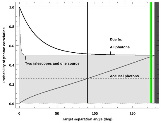
Figure 5.
Boundary conditions for the probability that detected photons are correlated in Equation (2), demanding that the fraction of acausal-pair photons is 100% at ; median situation shaded in grey.
Three different scenarios for viewing two quasars in a QM experiment can now be compared. A single site cannot effectively view quasar pairs with separations larger than about because extinction and observation quickly worsen (although less than exponentially) for each telescope with zenith airmass [16] and so incur an error that increases with separation up to some limiting observable airmass, typically under 2, as
for two telescopes at one site. These errors are assumed to be symmetric, without colour bias; thus, the absolute value is taken. The combined observational noise increases as
where is extinction, is the brightness of sky beyond the darkest possible brightness, is seeing (all at zenith); is the photometric error per n samples, and is the instrumental zeropoint error. Two sites separated by allow for larger viewable separations, because the zenith angle now has the form . In the third scenario, there are two telescopes at antipodal sites on the Earth, with the form , which might be in Hawai’i and southern Africa, for example. Such mid-latitude locations have 8 m class telescopes but do not allow for the simultaneous viewing of the same location on the sky, and there for must incur a penalty of at least in zeropoint calibration.
Imagine the smallest detectable correlation between two sources; that is, when , and the A-B colour difference per sample is twice the zeropoint limit of each instrument, ideally identical. Signal-per-exposure as a function (with parameters as shown in Table 1) is plotted in Figure 6: signal per exposure (top panel) is set by requiring that the on-axis (unseparated) sources cannot differ by more than this smallest measureable signal, which is provided here in magnitude units. The total observational noise, including zeropoint, background, and seeing for two sites separated by 90 degrees on the Earth, is also shown (bottom panel); the other geometries are shown as shaded regions, i.e., two telescopes at one site or two sites at antipodes (white curve) incurring twice the zeropoint noise, as they cannot be directly cross-calibrated. No observational scenario could do better than about noise per sample due to the zeropoint of real systems (roughly 1% photometry), even at a single site. A tradeoff (not shown) is required for sites with a separation of larger than 90 degrees, leading to a compromise between these two previous scenarios. This last scenario is that of the Gemini Observatory, with twin telescopes situated at a separation of about in great-circle distance.

Table 1.
Values of Parameters Used in Model.
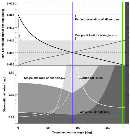
Figure 6.
Minimally detectable correlated signal per sample (top panel) for identical instruments and total observational noise (bottom panel), including zeropoint, photometric error per sample, seeing, and sky background, for two telescopes at one site and two sites separated by 90 degrees on the Earth (single exposure: light grey; 3000 samples: dark grey) or two sites at antipodes (thick white curve).
3. Observations
Gemini provides a suitable dataset for the demonstration of the search, as it operates identical high-framerate (up to ), low-noise, 1024 by 1024, Electron-Multiplying, Charge-Coupled Device (EMCCD) optical imagers ‘Alopeke and Zorro: dual-channel photometers, splitting flux into a blue (centred at , wide) and red (, ) passbands [17]. Installed in 2018, these are normally utilized (independently) in speckle interferometry, although the recorded limited-vision raw images are uncorrected. A typical set of four images is shown in Figure 7. The observations made using either instrument are normally a long sequence of 1000 exposures; the fast readout electronics allow for nearly integrations to be achieved, each timestamped to within microseconds. The absolute accuracy of the sequences is better than . The public archive was searched for serendipitous, simultaneous observations when both ‘Alopeke and Zorro obtained sequences starting within 5 s of each other. Four cases of three sets of observations of two bright stars (a total of twelve observations, listed by start time in Table 2) were found that met these timing restrictions, with the assurance that a loss of no more than 10% of the combined dataset was obtained. Equivalently, each has more than a 90% overlapping period of simultaneous observations.
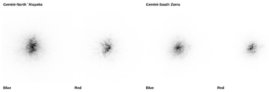
Figure 7.
Sample images from the Gemini ‘Alopoke/Zorro dataset with blue and red filters. These are the simultaneous integrations of two bright stars, one from the North and one from the South.
Table 2.
Stars imaged simultaneously for three minutes, each with Gemini ‘Alopeke and Zorro.
4. Analysis and Results
Aperture photometry was carried out on all images; a 5 arcsec synthetic aperture was applied, with a 1 arcsec-wide annulus surrounding it to obtain a sky estimate. A custom IDL code was written to perform this, which also generated the statistics for the combined data over the full 60 s of each sequence. The difference in flux for blue-red is the colour; this was converted to an AB magnitude via the published bandpasses and throughputs for the instruments, with close to 90% for blue and 70% for red.
This photometry was then converted to a difference relative to the standard deviation of the colour for the whole sequence; hence, it was reported as the std. dev. from the mean, as defined in Section 2.1. The results for one sequence are shown in Figure 8; that is, the A-B colour of the two stars in each frame. The chosen convention was that the object labelled A was that observed with ‘Alopeke and object B was that observed with Zorro. A linear fit for colour over the sequence was also subtracted to ensure that no trend was due to airmass changes, although this was found to have a negligible effect, well under 1%. The grey band in Figure 8 delineates 1 std. dev. above and below the slope-corrected mean. The resulting distributions are shown in Figure 9; both show one individual sequence of 60 s (left shows those from the same sequence as shown in Figure 8), and the combination of all 12 available observations is shown on the right; both of these are indistinguishable from the Gaussian (dashed curve) normalized to the same peak.
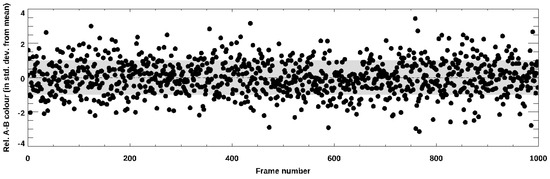
Figure 8.
Sample A-B colour photometry for one 1000-sample sequence of ‘Alopeke/Zorro data. This is the first sequence from the data of 9 October 2019.
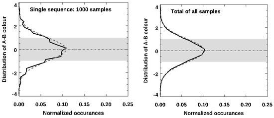
Figure 9.
Colour distributions for ‘Alopeke/Zorro data; for the 1000-frame sequence in Figure 8 (left panel) and for all 12 available archival observations (right panel) for a total of 12,000 samples.
An auto-correlation analysis identical to that described in Section 2.2 was also carried out, which confirms the random nature of the observed colours, as shown in Figure 10. Shifts of up to 5 s were allowed; the vertical dotted line indicates the time period during which the two local instrument clocks could be out of sync; there is no evidence of an improved correlation within that window. It is perhaps no surprise that the simultaneous colours of these stars are random, but it is still a useful excercise. That is because although these observations were undertaken at 0.06 s cadence, ‘Alopeke/Zorro are capable of 0.01 s exposures—shorter than the telescope-to-telescope light-travel time—as will be shown in the next section, which can allow for a test to be conducted for two quasars, which are both much fainter, but still provide sufficient photons to obtain an image at the highest framerate.
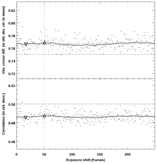
Figure 10.
Auto-correlation of ‘Alopeke/Zorro data in Figure 8. No detectable correlation is seen, allowing for shifts of up to for different start times (Zorro precedes ‘Alopeke) and ensuring the accuracy of the clock.
Finding Quasar Pairs to Complete a True Acausal–Photons Correlations Test
A software tool was developed to predict where pairs of quasars with the potentially observable and exploitable A-B colour signal of Section 2.1 might be found. It incorporates the expected noise limitations imposed at different sites and instrument properties (telescope aperture, framerate, and throughputs), as in Section 2.3, and then reports an SNR for those selected quasar pairs, based on catalogued brightnesses. The code can be set for Gemini (8.1 m apertures, geographic coordinates) and calculates the visibility of sources for the upcoming year and outputs a target list indicating the best night during that time. It can also restrict the allowed sky-offsets from a single object (for example, a calibration star) to be simultaneously visible at both sites on that night. The best time in the night is when both targets are at the lowest combined airmass for both sites, where both sources reach their highest ascension in both the North and South skies. The outputs are the target names for each of the two selected telescope sites, appending A and B with the convention that target A is rising and B is setting on the best night. This program is called PDQ (Predict Different Quasars), written in IDL, and is freely available via GitHub. The target list remains unvetted in this version of the code: neither the brightness of the quasars nor their redshifts are verified. A sample is listed in Table 3. Manual checking with slightly relaxed settings does find some suitable pairs that are bright enough to image with ‘Alopeke/Zorro.
Table 3.
Potential acausal quasar pairs that are visible for over two weeks with Gemini ‘Alopeke and Zorro.
Using the results from Section 4 on bright stars for comparison, the tool’s output is plotted in Figure 11: A-B observed-colour SNR for 3000 samples at 50 Hz. Alopeke/Zorro results are indicated by black-outlined stars; all others show the 18.5 R-mag and brighter quasars selected from the MILLIQUAS sample [12]; either (the mean sample reshift) separated by , or each has a (possibly photometric) redshift of ; those with a separation of are indicated by open down-pointing triangles. At all smaller separation angles, these are indicated by the minimal fraction of acausal photons per sample (dark grey filled circles) and causal (black). Where these would be visible to both telescopes, they are outlined by a grey circle; a black square indicates when it is, in fact, the same source, with zero separation. Coloured and shaded regions indicate the expected model-SNR limits for fair-sampling at other telescope site choices (Equation (2), with ): light grey is a limiting case if a single telescope has a field of view over the whole sky; blue denotes a single site with two telescopes; green indicates two sites with exactly separation on Earth; yellow indicates antipodal sites. There is an upper limit (for separation) from the model at 50 Hz, but the flux matches that of the observed stars (dashed curve).
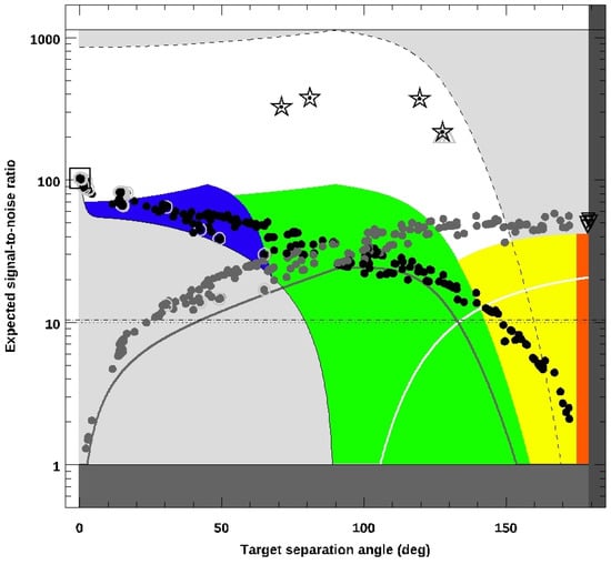
Figure 11.
Predicted A-B colour SNR for acausal photons (filled grey circles) from quasar pairs with Gemini ‘Alopeke and Zorro, as found with the PDQ software, plotted for instances when objects are visible for at least two weeks; the same is also shown for the causal fraction of photons (filled black circles), where the down-pointing triangles are for , acausal quasar pairs. For comparison, up-pointing triangles are a transitional case at peak SNR photons (but not fully acausal) near separation for 10,000 samples of , quasars; open circles flag those cases that could be observed by either site; an open square indicates both telescopes are observing one source (causal, with the same brightness as the acausal pairs); open stars denote the stellar sources that were previously observed by Gemini with 3000 samples each. The outer grey-shaded boundary shows the model results for fair-sampling (indistinguishable between causal and acausal photons; equation 2 shows ) and -separated sites and sources; sources (green), a single site (blue), and two antipodal sites (yellow) were obtained via the model presented in Section 2. Notice that, on optimal nights, Gemini provides the necessary conditions for viewing fully acausal sources (red), with an SNR similar to that of the antipodal sites.
Two further outputs help to visualize the orientation of the potential targets on the sky, and possible scheduling of observations: Figure 12 is a plot of right ascension and a declination of the targets displayed in Figure 11 as being visible in the coming year. Note the East–West alignment of acausal quasar pairs that are separated by (down-pointing tringles, with red filled circles). For comparison, the previously observed stars are shown; a black central dot indicates those viewed from Gemini South. In Figure 13, the polar projections of the visibility of the targets are shown for Gemini South (left) and Gemini North (right); again, it is clear that suitable acasual quasar pairs are visible towards the low eastern horizon (Gemini South) and western sky (Gemini North) simultaneously.
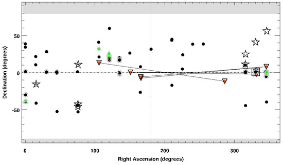
Figure 12.
Source pairs on the sky; symbols are those shown in Figure 11; here, the acausal quasar pairs are connected by a thin black line segmment; the South (B) star of the pair is indicated by a central black dot.
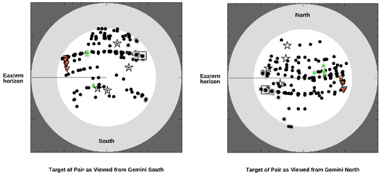
Figure 13.
Same as Figure 12, in polar projection from the zenith, as each is best viewed from either Gemini North or South at the lowest combined airmasses: a preferential East–West alignment is evident.
5. Summary and Conclusions
True random-number generation can be demonstrated via high-framerate photometric observations of quasar pairs that are separated by angles on the sky that make them inaccessible to any single ground-based observatory site. When apart, and each at , their emitted photons are acausal: no signalling between the sources could have spoiled the independence of a Bell-test setting procedure. So far, no such observations have been undertaken, and thus this is not proved. An analysis was carried out that sets boundaries on how observably correlated those two sources might be and the statistical signature of detecting that correlation relative to local noise sources. Simulated data were generated, and then an analytic model was used to compare among telescopes in three potential observing scenarios for any two observatory sites. It was found that two 8 m class telescopes at good sites at over separation on Earth are able, at reasonable observational limits and choices of optical bandpasses, and at high but practical camera framerates of , to to achieve a suitable SNR to overcome the seeing and sky-noise conditions, and therefore to rule out correlated noise ruining observations of suitable quasar pairs in QM tests. Details of the experimental procedures are left for other work.
To demonstrate the observational method and the utility of Gemini for the task, archival observations of four sets of bright star pairs obtained simultaneously (and serendipitously) in two bandpasses with ‘Alopeke/Zorro were presented. These do not meet the required framerate, obtained at only , but the necessary sampling speed is obtainable with this instrumental setup at its highest setting, . This also provides a calibration of the achievable SNR; the described model can extrapolate to fainter quasars observed at that framerate: typical sky conditions at the Gemini sites suggest that acausal 18.5 mag quasars can achieve an SNR of 50 in 3000 samples, ruling out correlations that are sufficient to spoil a QM test lasting minutes. Finally, a tool for finding suitable quasars to carry out such an observation and confirm there is no detectable correlation at the required framerate was presented, with example results obtained after running this PDQ code set for observations with Gemini ‘Alopeke/Zorro. It was found that several potential quasar pairs could be visible in the coming semesters, and so actual observations with Gemini may be considered. In the meantime, that code is freely provided via GitHub for the community, for example, when planning further QM tests.
Funding
This research received no external funding.
Data Availability Statement
All data discussed herein are freely available via public archives using the links indicated in the text, and their references. The data are also all downloadable from https://github.com/ericsteinbring/PDQ (accessed on 1 April 2025) in formatted data tables, together with the analysis code, written in IDL. In its default settings, that code generates the figures shown here.
Acknowledgments
I gratefully acknowledge the helpful comments from the anonymous referees, which improved the manuscript. This research used the facilities of the Canadian Astronomy Data Centre operated by the National Research Council of Canada with the support of the Canadian Space Agency. Archival observations employed the High-Resolution Imaging instruments ‘Alopeke and Zorro, funded by the NASA Exoplanet Exploration Program and built at the NASA Ames Research Center by Steve B. Howell, Nic Scott, Elliott P. Horch, and Emmett Quigley. ‘Alopeke and Zorro were mounted on the Gemini North and South telescopes of the international Gemini Observatory, a program of NSF NOIRLab, which is managed by the Association of Universities for Research in Astronomy (AURA) under a cooperative agreement with the U.S. National Science Foundation on behalf of the Gemini partnership: the U.S. National Science Foundation (United States), National Research Council (Canada), Agencia Nacional de Investigación y Desarrollo (Chile), Ministerio de Ciencia, Tecnología e Innovación (Argentina), Ministério da Ciência, Tecnologia, Inovações e Comunicações (Brazil), and Korea Astronomy and Space Science Institute (Republic of Korea).
Conflicts of Interest
The author declares no conflicts of interest.
Abbreviations
The following abbreviations are used in this manuscript:
| AGN | Active Galactic Nucleus |
| AO | Adaptive Optics |
| IDL | Interactive Data Language |
| NIR | Near Infrared |
| QM | Quantum Mechanics |
| SNR | Signal-to-Noise Ratio |
References
- Einstein, A.; Podolsky, B.; Rosen, N. Can Quantum-Mechanical Description of Physical Reality Be Considered Complete? Phys. Rev. 1935, 47, 777. [Google Scholar] [CrossRef]
- Bell, J.S. On the Einstein Podolsky Rosen Paradox. Physics 1964, 1, 195. [Google Scholar] [CrossRef]
- Rosenfeld, W.; Burchardt, D.; Garthoff, R.; Redeker, K.; Ortegel, N.; Rau, M.; Weinfurter, H. Event-Ready Bell Test Using Entangled Atoms Simultaneously Closing Detection and Locality Loopholes. Phys. Rev. Lett. 2017, 119, 010402. [Google Scholar] [CrossRef] [PubMed]
- Friedman, A.S.; Kaiser, D.I.; Gallicchio, J. The Shared Causal Pasts and Futures of Cosmological Events. Phys. Rev. D 2013, 88, 044038. [Google Scholar] [CrossRef]
- Gallicchio, J.; Friedman, A.S.; Kaiser, D.I. Testing Bell’s Inequality with Cosmic Photons: Closing the Setting-Independence Loophole. Phys. Rev. Lett. 2014, 112, 110405. [Google Scholar] [CrossRef] [PubMed]
- Handsteiner, J.; Friedman, A.S.; Rauch, D.; Gallicchio, J.; Liu, B.; Hosp, H.; Kofler, J.; Bricher, D.; Fink, M.; Leung, C.; et al. Cosmic Bell Test: Measurement Settings from Milky Way Stars. Phys. Rev. Lett. 2017, 118, 060401. [Google Scholar] [CrossRef] [PubMed]
- Wu, C.; Bai, B.; Liu, Y.; Zhang, X.; Yang, M.; Cao, Y.; Wang, J.; Zhang, S.; Zhou, H.; Shi, X.; et al. Random Number Generation with Cosmic Photons. Phys. Rev. Lett. 2017, 118, 140402. [Google Scholar] [CrossRef] [PubMed]
- Leung, C.; Brown, A.; Nguyen, H.; Friedman, A.S.; Kaiser, D.I.; Gallicchio, J. Astronomical Random Numbers for Quantum Foundations Experiments. Phys. Rev. A 2018, 97, 042120. [Google Scholar] [CrossRef]
- Rauch, D.; Handsteiner, J.; Hochrainer, A.; Gallicchio, J.; Friedman, A.S.; Leung, C.; Liu, B.; Bulla, L.; Ecker, S.; Steinlechner, F.; et al. Cosmic Bell Test Using Random Measurement Settings from High-Redshift Quasars. Phys. Rev. Lett. 2018, 121, 080403. [Google Scholar] [CrossRef] [PubMed]
- Clauser, J.F.; Horne, M.A.; Shimony, A.; Holt, R.A. Proposed Experiment to Test Local Hidden-Variable Theories. Phys. Rev. Lett. 1969, 23, 880. [Google Scholar] [CrossRef]
- Friedman, A.S.; Guth, A.H.; Hall, M.J.W.; Kaiser, D.I.; Gallichio, J. Relaxed Bell Inequalities with Arbitrary Measurement Dependence for Each Observer. Phys. Rev. A 2019, 99, 012121. [Google Scholar] [CrossRef]
- Flesch, E.V. The Million Quasars (Milliquas) Catalogue, V8. Open J. Astrophys. 2023, 6, 49. [Google Scholar] [CrossRef]
- Steinbring, E. A Star-Forming Shock Front in Radio Galaxy 4C+ 41.17 Resolved with Laser-Assisted Adaptive Optics Spectroscopy. Astron. J. 2014, 148, 10. [Google Scholar] [CrossRef]
- Li, M.-H.; Wu, C.; Zhang, Y.; Liu, W.-Z.; Bai, B.; Liu, Y.; Zhang, W.; Zhao, Q.; Li, H.; Wang, Z. Test of Local Realism into the Past without Detection and Locality Loopholes. Phys. Rev. Lett. 2018, 121, 080404. [Google Scholar] [CrossRef] [PubMed]
- Mudd, D.; Martini, P.; Zu, Y.; Kochanek, C.; Peterson, B.M.; Kessler, R.; Davis, T.M.; Hoormann, J.K.; King, A.; Lidman, C.; et al. Quasar Accretion Disk Sizes from Continuum Reverberation Mapping from the Dark Energy Survey. Astrophs. J. 2018, 862, 123. [Google Scholar] [CrossRef]
- Kasten, F. A New Table and Approximation Formula for the Relative Optical Air Mass. Arch. Meteorol. Geophys. Bioklimatol. Ser. B 1965, 14, 206. [Google Scholar] [CrossRef]
- Scott, N.J.; Howell, S.B.; Gnilka, C.L.; Stephens, A.W.; Salinas, R.; Matson, R.A.; Furlan, E.; Horch, E.P.; Everett, M.E.; Ciardi, D.R.; et al. Twin High-Resolution, High-Speed Imagers for the Gemini Telescopes: Instrument Description and Science Verification Results. Front. Astron. Space Sci. 2021, 8, 716560. [Google Scholar] [CrossRef]
Disclaimer/Publisher’s Note: The statements, opinions and data contained in all publications are solely those of the individual author(s) and contributor(s) and not of MDPI and/or the editor(s). MDPI and/or the editor(s) disclaim responsibility for any injury to people or property resulting from any ideas, methods, instructions or products referred to in the content. |
© 2025 by the author. Licensee MDPI, Basel, Switzerland. This article is an open access article distributed under the terms and conditions of the Creative Commons Attribution (CC BY) license (https://creativecommons.org/licenses/by/4.0/).