Machine Learning to Simulate Quantum Computing System Errors from Physical Observations

Abstract

In the context of quantum computing, error correction remains a pivotal challenge, primarily due to imperfect gate operations and environmental interactions. This study introduces a machine learning-based method to simulate and analyze these errors. Utilizing a minimal scalable 2-Majorana-zero-mode (2-MZM) island model within a one-dimensional p-wave topological superconductor, this research employs a detailed Hamiltonian approach combined with a bosonic thermal bath interaction. The analysis is conducted using the Pauli master equation and Monte Carlo simulations. This work’s novel contribution lies in applying Boosted Decision Tree with Gradient boosting (BDTG) and Multi-Layer Perceptron (MLP) machine learning techniques. These methods, trained on Monte Carlo simulation data, showed proficiency in predicting the evolution of error probabilities in the quantum system. The results indicate a significant potential for machine learning to offer a more efficient alternative for simulating quantum computing errors, thereby contributing to developing more robust quantum computing systems.

1. Introduction

Since the experimental demonstration of early quantum computing prototypes [1,2,3], quantum computation has garnered significant attention as a disruptive computational paradigm. Among the foremost challenges in realizing practical quantum computation lays error correction [4]. Three principal error mechanisms plague quantum systems:

(i)

Imperfect quantum gate operations.

(ii)

Environmental decoherence through system–bath interactions.

(iii)

Discrepancies between theoretical designs and physical implementations.

These fundamental limitations necessitate the development of robust error correction protocols for future fault-tolerant quantum computers.

Topological quantum computing architectures [5] offer a promising approach to error mitigation through intrinsic topological protection. Of particular interest are Majorana zero modes (MZMs) in topological superconductor (TS) nanowires [6,7,8,9,10,11,12], which exhibit non-Abelian exchange statistics [13,14,15]. While MZM-based qubits benefit from topological protection via nonlocal encoding, they remain susceptible to quasiparticle poisoning [16], a decoherence mechanism inducing two distinct error types:

• Dephasing errors (X/Y Pauli errors) through computational subspace leakage.
• Phase errors (Z Pauli errors) via parity-violating transitions [17].

The Pauli master equation provides a robust framework for modeling open quantum systems in thermal environments [18,19], typically implemented through Monte Carlo (MC) simulations. However, such simulations incur substantial computational overhead, particularly for multi-qubit systems, motivating the exploration of alternative methodologies.

Recent advances in quantum error mitigation leverage machine learning techniques across diverse applications: Recurrent neural networks demonstrate capability in predicting quantum trajectories and reconstructing Hamiltonian parameters from real-time superconducting qubit measurements [20], while noise-aware circuit learning (NACL) frameworks optimize quantum circuit architectures against device-specific noise profiles derived from gate set tomography [21]. Deep learning approaches further enable the precise spectral characterization of qubit noise environments by analyzing two-pulse echo decay data [22], outperforming conventional spectral estimation methods. Neural network-enhanced Bayesian estimation protocols significantly improve quantum metrology precision under dephasing noise through adaptive experiment design [23]. Most notably, machine learning quantum error mitigation (ML-QEM) [24] achieves scalable noise suppression in 100-qubit systems through hybrid graph neural network architectures, reducing computational overhead compared to traditional zero-noise extrapolation techniques.

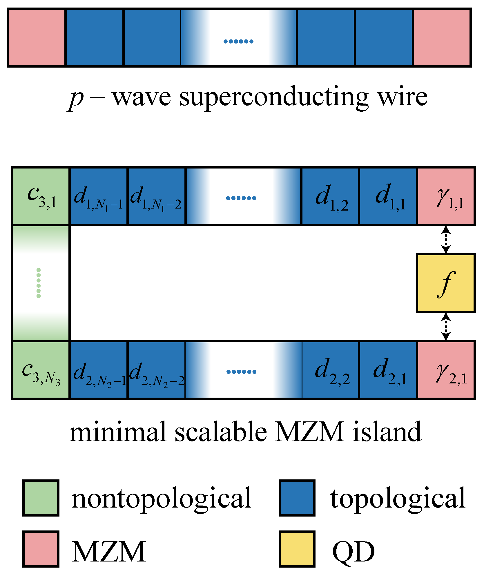
2. Minimal Scalable 2-MZM Island

Our model is a modified spinless variant of the standard 1D Kitaev chain, which is a canonical p-wave topological superconductor framework widely adopted in BDI symmetry studies. The Hamiltonian in real space is given by

$$H=-\mu \sum _{i=1}^N{c}_i^{†}{c}_i+\sum _{i=1}^{N-1}(-t{c}_i^{†}{c}_{i+1}+\Delta c_i{c}_{i+1}+\mathrm{h}.\mathrm{c}.),$$

(1)

where $c_i^{†}$ ($c_i$) is the spinless electron creation (annihilation) operators at site i. Here, $\mu$ is the chemical potential potential, t is the tunnelling strength, and $\Delta$ is the superconducting pairing potential. The model is topologically non-trivial when $\left|\mu \right|<2t$. In particular, the wire supports two MZMs at both ends in the case of $t=\Delta$ and $\mu =0$, which can be written in a compact form as

$$H_{\mathrm{top}}=i\Delta \sum _{i=1}^{N-1}{\gamma }_{2i}{\gamma }_{2i+1}=\Delta \sum _{i=1}^{N-1}(2d_j^{†}{d}_j-1),$$

(2)

where we use the Majorana operators ${\gamma }_{2i}=-i(c_i-c_i^{†})$ and ${\gamma }_{2i+1}=c_{i+1}+c_{i+1}^{†}$. The decoupled Majorana operators ${\gamma }_1$ and ${\gamma }_{2N}$ which satisfy $[H_{\mathrm{top}},{\gamma }_{j=1,2N}]=0$ are the MZMs at the ends of the wire. The quasiparticle operators are $d_j=({\gamma }_{2j}+i{\gamma }_{2j+1})/2$. The diagonal form of Equation (2) can be represented visually in a box form, as shown in Figure 1.

Scalable designs for quantum computation have been proposed by T. Karzig [25].

The key configuration of these designs is the MZM island, consisting of p-wave topological superconducting wires and quantum dots (QDs). MZMs in these designs are quasiparticle-poisoning-protected since the relatively large charging energy protects the fermion parity of the islands. However, the parity-preserving quasiparticle excitation can still lead to the dephasing of MZMs.

Let us consider a minimal scalable MZM island, which can also be represented in a box form, shown in Figure 1. The island can be decomposed into four parts: two topological bulk segments (colored blue) with two MZMs (colored red), a nontopological backbone (colored green), and a quantum dot (colored yellow). The grounded Hamiltonian of the island is given by

$$H_{\mathrm{island}}=H_1+H_2+H_3+H_{\mathrm{QD}}+H_T,$$

(3)

with

$$\begin{array}{cc}\hfill H_1& ={\Delta }_1\sum _{i=1}^{N_1-1}(2d_{1,i}^{†}{d}_{1,i}-1)\hfill \end{array}$$

(4)

$$\begin{array}{cc}\hfill H_2& ={\Delta }_2\sum _{i=1}^{N_2-1}(2d_{2,i}^{†}{d}_{2,i}-1)\hfill \end{array}$$

(5)

$$\begin{array}{cc}\hfill H_3& =\mu \sum _{i=1}^{N_3}{c}_{3,i}^{†}{c}_{3,i}+\sum _{i=1}^{N_3-1}(t{c}_{3,i}^{†}{c}_{3,i+1}+\mathrm{h}.\mathrm{c}.)\hfill \end{array}$$

(6)

$$\begin{array}{cc}\hfill H_{\mathrm{QD}}& ={\epsilon }_0{f}^{†}f\hfill \\ \hfill H_{\mathrm{T}}& =H_{\mathrm{T},13}+H_{\mathrm{T},23}+H_{\mathrm{T},\mathrm{QD}1}+H_{\mathrm{T},\mathrm{QD}2}\hfill \end{array}$$

(7)

$$\begin{array}{cc}\hfill & =t_{13}{d}_{1,N_1-1}^{†}{c}_1+t_{23}{d}_{2,N_2-1}^{†}{c}_1\hfill \end{array}$$

(8)

$$\begin{array}{cc}\hfill & +t_{\mathrm{QD}1}{\gamma }_{1,1}^{†}f+t_{\mathrm{QD}2}{\gamma }_{2,1}^{†}f+\mathrm{h}.\mathrm{c}.\hfill \end{array}$$

(9)

where $H_1$ and $H_2$ are the Hamiltonians of the topological bulk segments. Two topological bulk segments support four MZMs. However, an ingenious design of the island is that the two MZMs near the backbone side are hybridized, which requires that the width of the island (i.e., the size of the backbone) is shorter than the superconducting coherence length. Only two MZMs, ${\gamma }_{1,1}$ and ${\gamma }_{2,1}$, remain. The hybridization gives rise to an ordinary finite-energy Dirac fermion, which is regarded as one of the green boxes in Figure 1. The Hamiltonian $H_3$ contains the tunneling terms (with tunneling amplitude t), which means the quasiparticle can tunnel on the backbone. The spin freedom of the noninteracting QD Hamiltoonian $H_{\mathrm{QD}}$ can be neglected since the bulk segments coupling to the QD are spinless (or polarized). In the tunneling Hamiltonian $H_T$, the parameters $t_{13}$ and $t_{23}$ are the tunneling amplitudes between the bulk segments and the backbone. $t_{\mathrm{QD}1}$ and $t_{\mathrm{QD}2}$ are unbinding amplitudes between the bulk segments and the QD. The overall charging energy $H_C$ of the island is relatively large and would not be changed if only the parity-preserving quasiparticle excitation is under consideration here. Hence, the change in the island’s energy is only determined by the island’s grounded Hamiltonian.

We introduce a bosonic thermal bath interaction,

$$H_I=\sum _{\alpha =1,2}\sum _i^{N_{\alpha }}\lambda b_{\alpha ,i}\otimes (2c_{\alpha ,i}^{†}{c}_{\alpha ,i}-1),$$

(10)

where $\lambda$ is the coupling strength and $c_{\alpha ,j}^{†}$ are the spinless electron operators in the bulk segment $\alpha$ at site j. The bosonic operators $b_{\alpha ,j}$ locally interact with the electron at site j. This interaction can be regarded as quantum fluctuations of the chemical potential. The bosonic bath is trivial on the nontopological backbone but leads to the parity-preserving quasiparticle excitation on the bulk segments $(\alpha =1,2)$. The state of the open system depending on the time t is described by the Pauli master equation,

$${\displaystyle \frac{\mathrm{d}}{\mathrm{d}t}}P(n,t)=\sum _m\left[W\left(n\right|m\left)P\right(m,t)-W(m\left|n\right)P(n,t)\right],$$

(11)

where $P(n,t)$ is the population of a state, $\left|n\right.〉$, which is defined as the occupation state of the box representation in Figure 1. Each box is either an occupied or an unoccupied fermionic state. $W\left(n\right|m)$ is the transition rate from the state $\left|m\right.〉$ to $\left|n\right.〉$ and given by

$$W\left(n\right|m)=\gamma (\Delta ϵ){\left|\left.〈m\right|A_{\eta }^{\sigma }(\Delta ϵ)\left|n\right.〉\right|}^2,$$

(12)

where $\Delta ϵ={ϵ}_m-{ϵ}_n$ is the energy difference between the states $\left|m\right.〉$ and $\left|n\right.〉$. The jump operators $A_{\eta }^{\sigma }(\Delta ϵ)$ describe the behaviors of the quasiparticle excitations in the cases of $\sigma$ which are provided in Appendix A, with $\eta =\{\mathrm{hopping},\mathrm{creation},\mathrm{annihilation}\}$. Noting that the MZMs near the backbone are hybridized, the jump operators $A_{\eta }^{\alpha ,N_{\alpha }}$ are excluded in our discussion. The bath spetral function $\gamma \left(\omega \right)$ is given by

$$\gamma \left(\omega \right)=\kappa \left|{\displaystyle \frac{\omega }{1-exp(-\beta \omega )}}\right|,$$

where $\kappa$ is the couping constant and $\beta =1/\left(k_{\mathrm{B}}T\right)$ is the reciprocal of the thermodynamic temperature with $k_{\mathrm{B}}$, the Boltzmann constant.

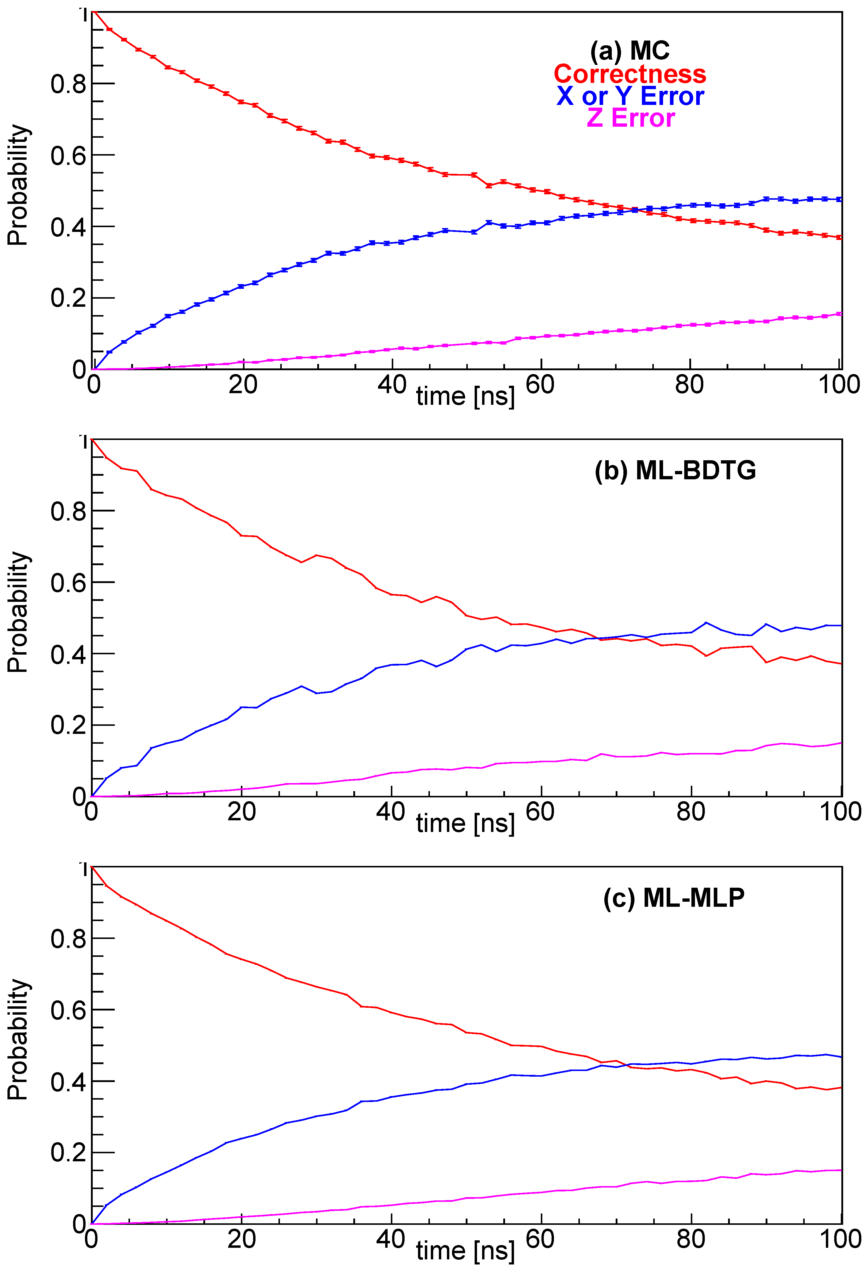
Monte Carlo Study of 2-MZM Island

In this section, we discuss the lifetime of the MZMs on the 2-MZM island. We use the standard residence time Monte Carlo algorithm to study the Pauli master Equation (11) with the following steps:

1.

Initialize the relevant parameters and initialize the system to the state $\left|m\right.〉$.

2.

Determine the time $\delta t=-ln\left(u\right)/\left[{\sum }_{n}W\left(n\right|m)\right]$, where u is a random number uniformly distributed in the interval $(0,1)$.

3.

Update the simulation time to $t=t+\delta t$ and if $t+\delta t<t_{\mathrm{sim}}$, go to step 4, or go directly to step 5.

4.

Implement the jump operators at random in the system according to the transition rate $W\left(n\right|m)$.

5.

Record the states of the two MZMs.

We can repeat the Monte Carlo algorithm above enough times so that we can obtain the probabilities of different errors. For simplicity, we consider a symmetrical island whose upper part is the same as the lower part with ${\Delta }_1={\Delta }_2=\Delta$; $N_1=N_2=N$; $t_{13}=t_{23}=t_{\mathrm{B}}$; and $t_{\mathrm{QD}1}=t_{\mathrm{QD}2}=t_{\mathrm{QD}}$.

The parameters we take here are shown in

Table 1. Key simulation parameters (units of $\Delta$; $\beta =3/\Delta$).

t	${\mathit{t}}_{\mathit{B}}$	${\mathit{t}}_{\mathit{QD}}$	$\mathit{\mu }$	${\mathit{\epsilon }}_0$	$\mathit{\kappa }$	N (Site)	${\mathit{N}}_3$ (Site)
2	5	2	10	2	$2\times {10}^{-4}$	3009	6

.

The system is defined by the following quantities:

• The length of the bulk segments, $L_{bulk}$;
• The chemical potential of the backbone, $\mu$;
• The induced superconducting gap, $|\Delta |$;
• The effective orbital energy of the quantum dot, h;
• The charging energy of the quantum dot, ${ϵ}_c$;
• The induced charge on the island, $n_g$;
• The transition amplitude in the Pauli master equation, $A_j$;
• The inverse temperature in the thermal bath, $\beta$.

The quality of the MZM system can be characterized by the probability of obtaining a final status with no error, i.e., the correct status, $P_C$. The probabilities of the X/Y and Z error in the final status are $P_{XY}$ and $P_Z$ respectively. Obviously, $P_C+P_{XY}+P_Z=1$.

To simulate the impact of the parameter values on the final probability, one can generate many Monte Carlo (MC) events [26] for each set of parameters. The uncertainty of the error probability, which is calculated by the 68.3% confidence interval in the multinomial distribution, is anti-correlated to the Monte Carlo statistics [27]. To bring down the uncertainty to the percentage level for each set of parameters, the Monte Carlo statistics should be ${10}^4$. For instance, there should be ${10}^4$ results with no error out of $2\times {10}^4$ total simulations, and $P_C$ is 0.5 with the relative uncertainty ∼$\sqrt{{10}^4}/{10}^4=1\%$. If one wants to study a parameter range to obtain a high $P_C$, it requires a lot of computation power. In our case, nine parameters will affect the error probability. When we scan the parameter space and take 10 values for each parameter, we have ${10}^9$ sets of parameters. This requires ∼${10}^{13}$ simulations.

This section may be divided by subheadings. It should provide a concise and precise description of the experimental results, their interpretation as well as the experimental conclusions that can be drawn.

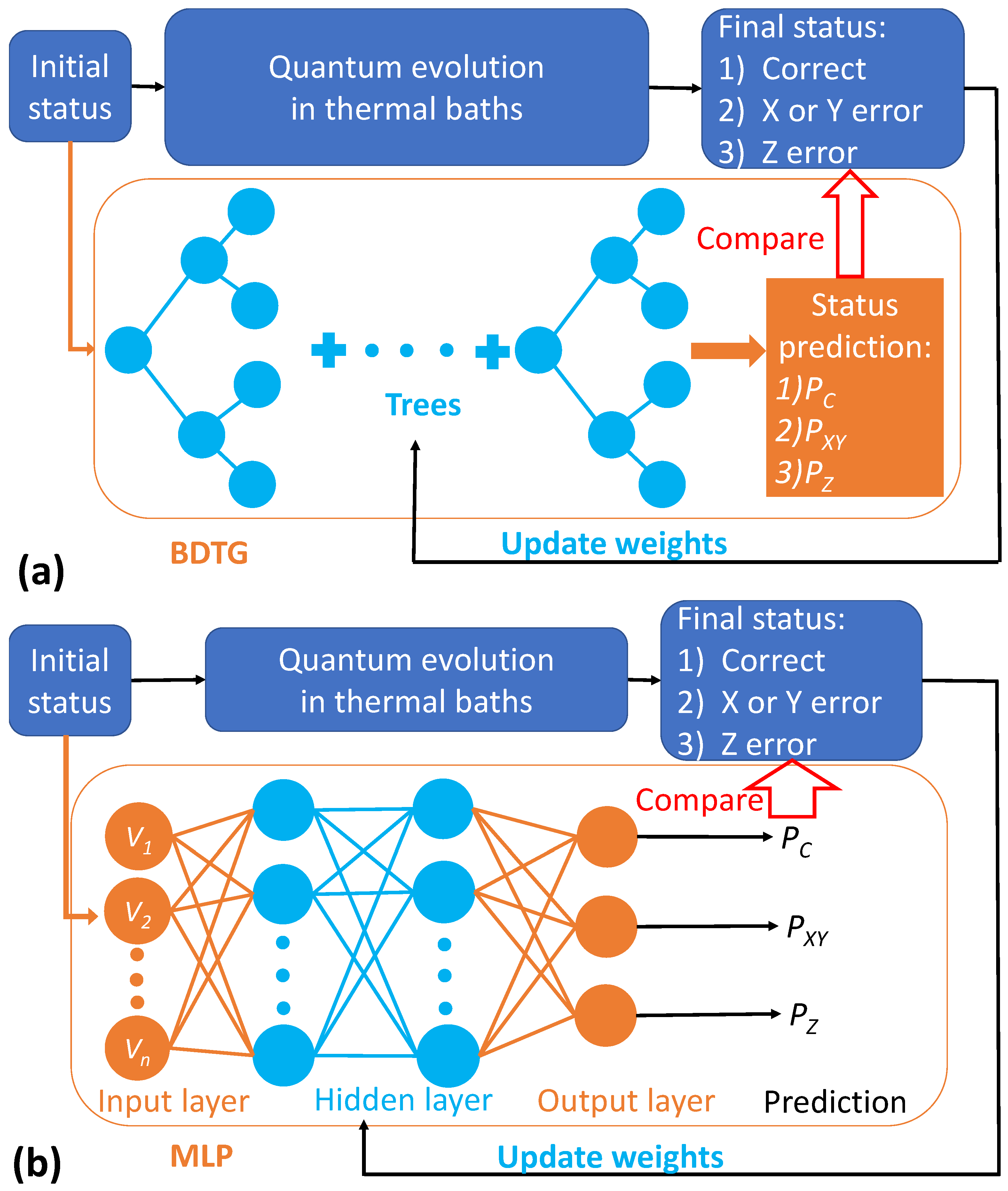
3. Machine Learning Methods

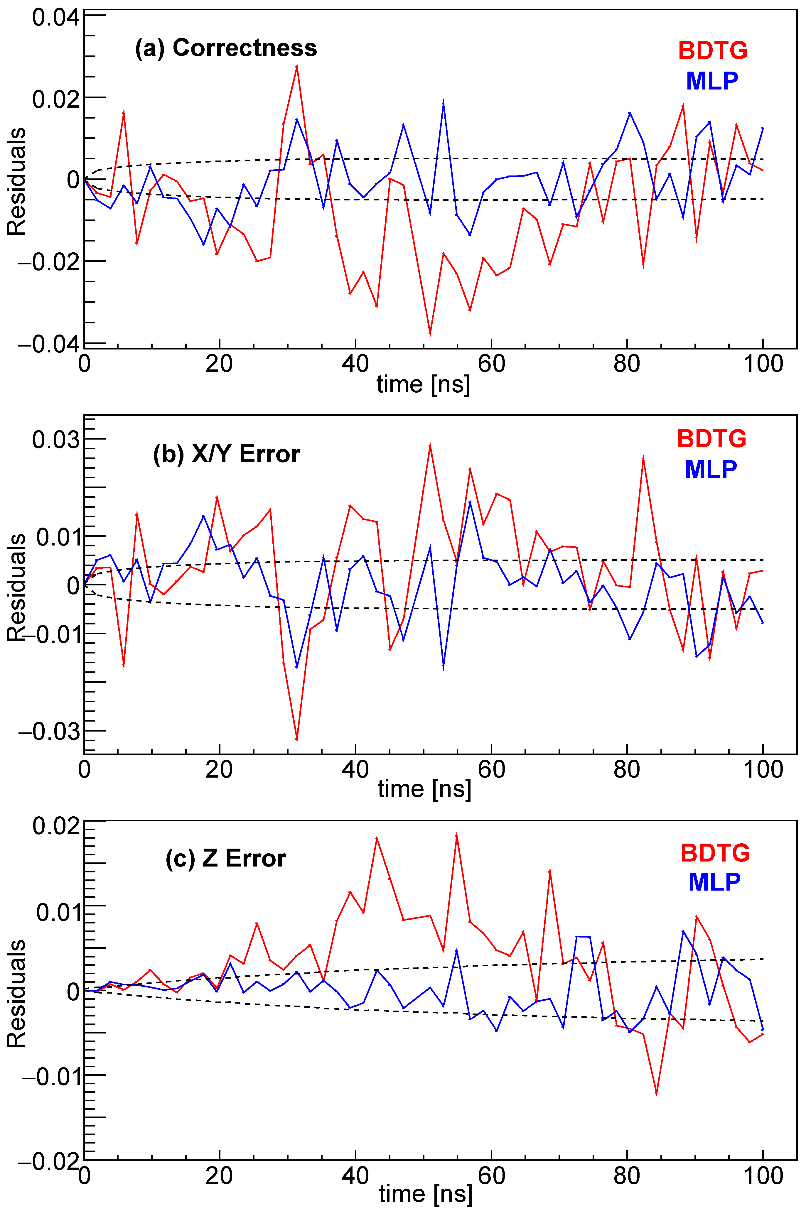
In the same system, different sets of parameters are correlated with each other. It is helpful to model this correlation for reducing computation load. Machine learning (ML) methods can provide us with these models. Probing the probability of quantum computing system error can be described as a typical classification problem.

The Boosted Decision Tree with Gradient boosting (BDTG) [28] and the Multi-Layer Perceptron (MLP) [29] techniques in the Toolkit for Multivariate Data Analysis (TMVA) package [30] were implemented in the study.

Before using this model, we needed to train these models with MC events. Figure 2 shows the flow charts of the model training of the BDTG and MLP methods. The ith MC event with the set of parameters $\mathit{V}$ went through quantum evolution after the time $\tau$ and error correction procedures. The final status ${\mathit{Stat}}_{\mathit{i}}$ could be presented by one of the three vectors:

$${\mathit{Stat}}_{\mathit{i}}=\left\{\begin{array}{cc}(1,0,0),\hfill & \mathrm{Correctness}.\hfill \\ (0,1,0),\hfill & \mathrm{X}\mathrm{or}\mathrm{Y}\mathrm{Error}.\hfill \\ (0,0,1),\hfill & Z\mathrm{Error}.\hfill \end{array}\right.$$

(13)

On the other hand, the model predicted the ith MC event with the set of parameters $\mathit{V}$ to have a final status probability:

$$P_{Sta{t}_i}=(P_C,P_{XY},P_Z).$$

(14)

In general, the loss function could be defined as

$$\mathcal{L}=\sum _i^N{(P_{Sta{t}_i}-Sta{t}_i)}^2.$$

(15)

A total of $2.5\times {10}^7$ MC events were generated for training and testing of the ML methods. The training process used half of the total events, i.e., $N=1.25\times {10}^7$, while the other half of the events were used for testing the models. The parameter ranges in the Monte Carlo simulations are provided in

Table 2. Parameter ranges in the Monte Carlo simulations.

Parameter	Minimum Value	Maximum Value
$L_{\mathrm{bulk}}$ (nm)	40	2504
$\mu$ ($\mathsf{\mu }$eV)	−900	−400
$|\Delta |$ ($\mathsf{\mu }$eV)	80	500
h ($\mathsf{\mu }$eV)	80	1200
${ϵ}_c$ ($\mathsf{\mu }$eV)	1200	18,000
$n_g$	0.02	0.3
$A_j$	0.1	1.5
$\beta$	0.002	0.03

.

In this study, two machine learning algorithms were implemented with systematically tuned hyperparameters to address quantum computing data classification. For MLP, hyperbolic tangent activation functions (NeuronType = tanh) were employed to capture nonlinearity, and input variables were standardized via normal transformation (VarTransform = N). The hidden layer dimensionality was dynamically defined as $N+5$ (where $N=9$ represents the number of input features), balancing representational capacity and architectural efficiency. Model training proceeded for 500 iterations (NCycles = 500), with validation metrics assessed every 10 epochs (TestRate = 10) to facilitate convergence monitoring (EpochMonitoring) and mitigate overfitting. Meanwhile, BDTG ensembles integrated 120 trees in the forest through gradient boosting (BoostType = Grad), regulated by a learning rate of 0.30 (Shrinkage = 0.30) for stable residual correction. Stochastic robustness was enhanced by a bootstrap aggregation scheme, sampling 60% of the training data in each boosting iteration (GradBaggingFraction = 0.6). The model’s complexity was controlled by cost-complexity pruning (PruneMethod = CostComplexity) with a pruning strength of 60 (PruneStrength = 60) and a maximum of five nodes per tree (NNodesMax = 5). Furthermore, Gini impurity minimization (SeparationType = GiniIndex) guided the splitting criterion, with 25 grid points in the variable range used in finding the optimal cut in node splitting to ensure effective yet discriminative partitions.

4. Discussion

To validate the ML methods, we compared the predictions of the ML methods to results calculated using MC simulation. Figure 3 shows that both the BDTG and MLP methods could correctly predict the trends of the time evolution of the error probabilities of the 2-MZM island system. Figure 3a includes the statistical uncertainties of MC events which follow multinomial distributions. The result from the MLP method is smoother compared to that from BDTG.

As shown in Figure 4, the residuals between BDTG (red curves) and MLP (blue curves) predictions relative to Monte Carlo simulations are presented for three observables: (a) correctness residuals, (b) X/Y positional error residuals, and (c) Z-direction error residuals. Both ML methods exhibit deviations within the Monte Carlo $1\sigma$ uncertainty band (black dashed lines) across the 0–100 ns time range. In general, MLP shows better performance than BDTG.

5. Conclusions

In this concise summary, we highlight the primary findings and implications of our study on simulating quantum computing errors using machine learning. Our approach, utilizing BDTG and MLP models trained on Monte Carlo simulation data, effectively predicted error probabilities in a minimal scalable 2-MZM island model. This method demonstrates a significant improvement in efficiency over traditional simulation techniques.

Our results underscore the potential of machine learning in enhancing quantum computing error analysis, offering a pathway to more robust quantum computing systems by addressing key challenges in error correction. This study lays a foundation for further exploration in applying machine learning to complex quantum systems, marking a step forward in the field of quantum computing.

References

1. Jones, J.A.; Mosca, M. Implementation of a quantum algorithm to solve Deutsch’s problem on a nuclear magnetic resonance quantum computer. J. Chem. Phys. 1998, 109, 1648–1653. [Google Scholar] [CrossRef]
2. Chuang, I.; Gershenfeld, N.; Kubinec, M. Experimental Implementation of Fast Quantum Searching. Phys. Rev. Lett. 1998, 80, 3408–3411. [Google Scholar]
3. Vandersypen, L.M.K.; Steffen, M.; Breyta, G.; Yannoni, C.S.; Sherwood, M.H.; Chuang, I.L. Experimental realization of Shor’s quantum factoring algorithm using nuclear magnetic resonance. Nature 2001, 414, 883–887. [Google Scholar] [CrossRef] [PubMed]
4. Stolze, J.; Suter, D. Quantum Computing—A Short Course from Theory to Experiment, 2nd ed.; Wiley: Hoboken, NJ, USA, 2008. [Google Scholar]
5. Kitaev, A.Y. Fault-Tolerant Quantum Computation by Anyons. Ann. Phys. 2003, 303, 2–30. [Google Scholar] [CrossRef]
6. Kitaev, A.Y. Unpaired Majorana fermions in quantum wires. Physics-Uspekhi 2001, 44, 131–136. [Google Scholar] [CrossRef]
7. Lutchyn, R.M.; Sau, J.D.; Das Sarma, S. Majorana Fermions and a Topological Phase Transition in Semiconductor-Superconductor Heterostructures. Phys. Rev. Lett. 2010, 105, 077001. [Google Scholar] [CrossRef] [PubMed]
8. Oreg, Y.; Refael, G.; von Oppen, F. Helical Liquids and Majorana Bound States in Quantum Wires. Phys. Rev. Lett. 2010, 105, 177002. [Google Scholar] [CrossRef]
9. Sarma, S.D.; Freedman, M.; Nayak, C. Majorana zero modes and topological quantum computation. NPJ Quantum Inf. 2015, 1, 15001. [Google Scholar] [CrossRef]
10. Nayak, C.; Simon, S.H.; Stern, A.; Freedman, M.; Das Sarma, S. Non-Abelian anyons and topological quantum computation. Rev. Mod. Phys. 2008, 80, 1083–1159. [Google Scholar] [CrossRef]
11. Sau, J.D.; Lutchyn, R.M.; Tewari, S.; Das Sarma, S. Generic New Platform for Topological Quantum Computation Using Semiconductor Heterostructures. Phys. Rev. Lett. 2010, 104, 040502. [Google Scholar] [CrossRef]
12. Lutchyn, R.M.; Bakkers, E.P.A.M.; Kouwenhoven, L.P.; Krogstrup, P.; Marcus, C.M.; Oreg, Y. Majorana zero modes in superconductor–semiconductor heterostructures. Nat. Rev. Mater. 2018, 3, 52–68. [Google Scholar] [CrossRef]
13. Alicea, J.; Oreg, Y.; Refael, G.; von Oppen, F.; Fisher, M.P.A. Non-Abelian statistics and topological quantum information processing in 1D wire networks. Nat. Phys. 2011, 7, 412. [Google Scholar] [CrossRef]
14. Ivanov, D.A. Non-Abelian Statistics of Half-Quantum Vortices in p-Wave Superconductors. Phys. Rev. Lett. 2001, 86, 268–271. [Google Scholar] [CrossRef]
15. Stone, M.; Chung, S.B. Fusion rules and vortices in px+ipy superconductors. Phys. Rev. B 2006, 73, 014505. [Google Scholar] [CrossRef]
16. Karzig, T.; Cole, W.S.; Pikulin, D.I. Quasiparticle Poisoning of Majorana Qubits. Phys. Rev. Lett. 2021, 126, 057702. [Google Scholar] [CrossRef] [PubMed]
17. Knapp, C.; Karzig, T.; Lutchyn, R.M.; Nayak, C. Dephasing of Majorana-based qubits. Phys. Rev. B 2018, 97, 125404. [Google Scholar] [CrossRef]
18. Pedrocchi, F.L.; Bonesteel, N.E.; DiVincenzo, D.P. Monte Carlo studies of the self-correcting properties of the Majorana quantum error correction code under braiding. Phys. Rev. B 2015, 92, 115441. [Google Scholar] [CrossRef]
19. Breuer, H.P.; Petruccione, F. The Theory of Open Quantum Systems; Oxford University Press: Oxford, UK, 2002. [Google Scholar]
20. Flurin, E.; Martin, L.S.; Hacohen-Gourgy, S.; Siddiqi, I. Using a Recurrent Neural Network to Reconstruct Quantum Dynamics of a Superconducting Qubit from Physical Observations. Phys. Rev. X 2020, 10, 011006. [Google Scholar] [CrossRef]
21. Cincio, L.; Rudinger, K.; Sarovar, M.; Coles, P.J. Machine Learning of Noise-Resilient Quantum Circuits. PRX Quantum 2021, 2, 010324. [Google Scholar] [CrossRef]
22. Wise, D.F.; Morton, J.J.; Dhomkar, S. Using Deep Learning to Understand and Mitigate the Qubit Noise Environment. PRX Quantum 2021, 2, 010316. [Google Scholar] [CrossRef]
23. Fiderer, L.J.; Schuff, J.; Braun, D. Neural-Network Heuristics for Adaptive Bayesian Quantum Estimation. PRX Quantum 2021, 2, 020303. [Google Scholar] [CrossRef]
24. Liao, H.; Wang, D.S.; Sitdikov, I.; Salcedo, C.; Seif, A.; Minev, Z.K. Machine learning for practical quantum error mitigation. Nat. Mach. Intell. 2024, 6, 1478–1486. [Google Scholar] [CrossRef]
25. Karzig, T.; Knapp, C.; Lutchyn, R.M.; Bonderson, P.; Hastings, M.B.; Nayak, C.; Alicea, J.; Flensberg, K.; Plugge, S.; Oreg, Y.; et al. Scalable designs for quasiparticle-poisoning-protected topological quantum computation with Majorana zero modes. Phys. Rev. B 2017, 95, 235305. [Google Scholar] [CrossRef]
26. Feng, G.H.; Chen, J.; Zhang, H.H. Monte Carlo studies of modified scalable designs for quantum computation. arXiv 2019, arXiv:1911.06755. [Google Scholar]
27. Tanabashi, M.; Hagiwara, K.; Hikasa, K.; Nakamura, K.; Sumino, Y.; Takahashi, F.; Tanaka, J.; Agashe, K.; Aielli, G.; Particle Data Group; et al. Review of Particle Physics. Phys. Rev. D 2018, 98, 030001. [Google Scholar] [CrossRef]
28. Friedman, J.H. Greedy Function Approximation: A Gradient Boosting Machine. Ann. Stat. 2001, 29, 1189–1232. [Google Scholar] [CrossRef]
29. Fukushima, K. Training multi-layered neural network Neocognitron. Neural Netw. 2013, 40, 18–31. [Google Scholar] [CrossRef]
30. Hoecker, A.; Speckmayer, P.; Stelzer, J.; Therhaag, J.; von Toerne, E.; Voss, H.; Backes, M.; Carli, T.; Cohen, O.; Christov, A.; et al. TMVA—Toolkit for Multivariate Data Analysis. arXiv 2009, arXiv:physics/0703039. [Google Scholar]
Figure 1. A box representation of the p-wave topological superconducting wire and the minimal scalable MZM island. The red boxes correspond to the MZMs γ 1 , 1 and γ 2 , 1 . The upper (lower) blue boxes correspond to the quasiparticles d 1 , i ( d 2 , i ) . The green boxes correspond to the electrons c 3 , i . The yellow box corresponds to the QD f.
Universe 11 00120 g001
Figure 2. Flow charts of quantum–classical hybrid computation frameworks. (a) Boosted Decision Tree with Gradient boosting (BDTG) architecture showing quantum error correction workflow. (b) Multi-Layer Perceptron (MLP) architecture demonstrating neural network parameter optimization. Dark blue elements represent quantum evolution and error correction processes (traditional Monte Carlo modules). Orange modules denote machine learning components with light-blue adjustable weight matrices.
Universe 11 00120 g002
Figure 3. Comparative analysis of error probability dynamics. (a) Monte Carlo (MC) simulation with traditional error propagation. (b) Machine learning–Boosted Decision Tree with Gradient boosting (ML-BDTG) prediction. (c) Machine learning–Multilayer Perceptron (ML-MLP) neural network estimation. Time evolution profiles were computed under identical quantum circuit conditions.
Universe 11 00120 g003
Figure 4. Residual comparisons of (a) correctness and (b) X/Y and (c) Z error probabilities between BDTG (red curves) and MLP (blue curves) predictions against Monte Carlo reference values. Black dashed lines indicate statistical uncertainties derived from MC simulations.
Universe 11 00120 g004