Abstract
We determine the interaction energy of electric monopole pairs, sources and sinks of a Coulombic field. These charges are represented by topological solitons of finite size and mass, described by a field of SO(3) rotations without any divergences. Such monopoles feel, at large distances, a pure Coulombic interaction. A crucial test for the physical interpretation of these monopoles is a classical running of the charge at small distances, expected from the finite soliton size. We investigate in detail a first observation of the increase in the effective charge at distances of a few soliton radii in this purely Coulombic system and compare it with the running of the coupling in perturbative QED.
1. Introduction
In Refs. [1,2], we proposed a dynamical model with only three degrees of freedom (dofs) for the dynamics of electrically charged monopoles represented by topological solitons, the model of topological particles (MTP). This model does not suffer from any singularities as Dirac’s magnetic monopoles and other classical field models do. Particles are identified by topological quantum numbers. One of them is the charge, topologically quantised in units of an elementary charge. Depending on the interpretation, the charges can be either electrical or magnetic after a dual transformation. They are referred to as charges because they exhibit Coulombic behavior. Masses of particles originate in field energy and opposite charges can cause annihilation. The model and its many predictions were extensively discussed in Ref. [2].
Magnetic monopoles were defined by Dirac in 1931 [3,4] as quantised singularities in the electromagnetic field. He found that their existence would explain the quantisation of electric charge, proven in Millikan’s experiments [5] but not explained by Maxwell theory [6]. Dirac monopoles have two types of singularities: the Dirac string, a line-like singularity connecting monopoles and antimonopoles, and the singularity in the centre of the monopole, a singularity analogous to the singularity of point-like electrons. Wu and Yang succeeded to formulate magnetic monopoles without the line-like singularities of the Dirac strings by using either a fibre-bundle construction with two different gauge fields [7], one for the northern and one for the southern hemisphere of the monopole, or by a non-abelian SU(2) gauge field in 3+1D [8,9]. The non-abelian Wu–Yang monopoles still suffer from the point-like singularities in the centre. There are monopole solutions without any singularity in the Georgi–Glashow model [10]: the ’t Hooft–Polyakov monopoles [11,12]. The Georgi–Glashow model, formulated in 3+1D, has 15 dofs, an adjoint Higgs field with three dofs and an SU(2) gauge field with field components. Only one dof is needed for the Sine–Gordon model [13], a model in 1+1D. It is most interesting that in addition to waves, it has kink and anti-kink solutions which interact with each other. The kink–antikink configurations are attracting and the kink–kink configurations are repelling. Obviously, the simplicity of the Sine–Gordon model inspired Skyrme [14,15,16,17,18] to create a model in 3+1D with a scalar SU(2)-valued field. Stable topological solitons (Skyrmions) emerge in that model with the properties of particles, interacting at short range. Because of the drastic difference between the short-range strong interaction and the long-range Coulomb interaction, the solitons of the Skyrme model have a completely different structure than the solitons of our model and the mathematical fields have a completely different interpretation despite their algebraic similarity. MTP was also inspired by the simplicity and physical content of the Sine–Gordon model; it was first formulated in [1]. It uses SO(3) degrees of freedom (dofs). SU(2) is the double covering group of SO(3) and is isomorphic to an S3. The dofs of SO(3) can therefore be related to a hemisphere of S3. The calculation with the matrices of SU(2) is simpler than the equivalent calculation with the matrices of SO(3). The only difference between the field configurations of SU(2) and SO(3) is that field configurations of SU(2) that differ only by a center element describe the same field configuration of SO(3). The hemisphere of S3 mentioned above is bounded by an , which is referred to as the equatorial sphere . The MTP vacuum has a twofold degeneracy on this equatorial sphere in order to describe the long-range Coulombic interaction. The relations of MTP to electrodynamics and symmetry breaking were discussed in [2,19].
In this article, we want to concentrate on numerical determinations of the interaction energy for a pair of charges, represented by soliton–antisoliton pairs and especially on the tiny deviations from pure Coulombic behaviour. Due to the non-existence of magnetic monopoles, comparisons to nature—the main duty of physics—are possible only for electric charges and the predictions of QED.
In Section 2, we repeat the formulation and some basic properties of the model; in Section 4, we show first results of the calculations and compare the results to perturbative QED. We find astonishing analogies of the short-distance behaviour of the interaction. In the Appendix A, we present the numerical formulation in cylindrical coordinates and show some informative diagrams.
2. Summary of MTP
As explained in Ref. [2], we use the SO(3) degrees of freedom (dofs) to describe electromagnetic phenomena. The calculations become simpler when using SU(2) matrices,
in Minkowski spacetime as field variables, where the arrows indicate vectors in the 3D algebra of su(2) and the basis vectors are represented by the Pauli matrices . The Lagrangian of MTP is
with
chosen so that topological solitons with a long-range Coulomb field are stable and lead to finite energy; see Ref. [2]. With the vector sign above the letters and , we indicate that these quantities are algebra elements of su(2), i.e., vectors in a three-dimensional Euclidean space, the tangential space of SU(2) at unity. This type of notation simplifies the calculations because the rules of vector algebra can be used. According to Equation (3), the curvature tensor is defined as an su(2)-valued area density, as the ratio of an infinitesimal area in the SU(2) target space to the corresponding area in Minkowski space.
Since the field strengths in electrodynamics refer to areas in spacetime, we come into contact with charges and their electromagnetic field by relating the electromagnetic field strength tensor to the dual of the curvature tensor ,
By using the dual curvature tensor, static electrons are described by the space–space components of the field strength tensor. For hypothetical magnetic monopoles, we would have to omit the dual transformation.
The twofold differentiability of the Q-field leads to the Maurer–Cartan equation
We can therefore write in the more general form
as it is known from differential geometry and its applications. The simpler expression (3) corresponds to a favorable choice of the local coordinate systems in the su(2) algebra.
3. Fields of Single Charges
The Q-field configurations of isolated charges are fundamental for understanding the Coulomb interaction. We choose these fields so that they define topologically stable solitons by the definition (2) of the Lagrangian. To simplify the formulation, we place the center of a soliton at the origin of our spatial coordinate system. The corresponding field value at the origin is formed by one of the two center elements of SU(2). To the far field of the solitons on the infinitely distant , we assign Q-values on the above-mentioned , for which the second term of the Lagrangian density vanishes. This term does not contain any derivatives, so it has the function of a potential energy density and defines the vacuum states of the model. This choice of field defines a homotopy group , a mapping of the onto the . As can be seen in (32) [2], the minimization of the effect for the real part of the soliton field Q results in a very simple relation
where r is the radial coordinate. The values therefore approach the doubly degenerate vacuum asymptotically with . We can align the imaginary part of the soliton field with the coordinate axes for simple representation by
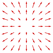
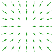
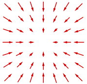
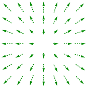
The four spherically symmetrical fields defined by the signs in the Equations (7) and (8) are shown graphically with vector arrows in the figures in Table 1. They are characterized by their simple hedgehog shape. The signs of the values are symbolized by the colors and dotted shafts of the arrows.

In the limiting case , all arrows have a length of 1 and the Q-field is essentially reduced to the -field. In the center, the singularity characteristic of point charges arises, which immediately shows that the integral Gauss law is exactly fulfilled. Each area enclosing the soliton center results in a full coverage of . The electric field strength defined as a non-Abelian field according to Equation (4) only has a non-vanishing component that points in the direction and becomes the Abelian field strength . This allows a charge number to be defined for the charge enclosed in the volume V with the surface
The hedgehog solutions (7) and (8) are characterised by a further quantum number, the number of coverings of the SU(2) manifold, the topological charge, well known from QCD and non-Abelian gauge theories:
Here, is the Jacobi determinant for the map of the three-dimensional space to . is the volume of ; therefore, describes a full covering. The hedgehog configurations cover only half of with different chirality resulting in . The magnitude of the topological charge can be defined as the spin quantum number
of any regular field configuration of the model.
The deviations from the behavior in Equation (7) provide a geometric explanation of why deviations from the Coulomb law of point charges are to be expected for finite at distances of some multiples of . For isolated solitons, the deviations can be determined analytically and show the internal non-Abelian structure. From the definition (3) follows in spherical coordinates
where and , are spherical unit vectors in the su(2) algebra. The non-Abelian electrical field strength results in
At this point, it is appropriate to mention the relationship to other investigations. In the limiting case , these expressions agree with the expressions given by Wu and Yang [8,9] for their non-Abelian description of point-like magnetic Dirac monopoles, except for the different charge. The value of the radial electric field strength also agrees with the regularization of the electric field strength of an electron proposed by Schwinger [20], which leads to an easily calculated rest mass of the regularized electron of . As is also relatively easy to calculate, the non-Abelian field strengths and and the potential energy density double this value to
the rest energy of isolated topologically stable solitons; see also Ref. [2] with more detailed calculations. The only known fundamental stable monopoles are electrons with a self-energy of MeV. A comparison leads to
a scale which is of the order of the classical electron radius . The four parameters and correspond to the natural scales of the four quantities of length, time, mass and charge of the SI, of the Système international d’unités, which are involved in this model. If the value ℏ is calculated from quantum mechanical effects, Equation (14) can be interpreted as a relation between and ℏ.
We know from electron–positron scattering experiments that the fine structure constant depends on the strength of the collisions between the particles. So far, there is only one theory that explains such an effect in agreement with the experiment. In QED, this effect is called “running coupling” and is calculated with the help of perturbation theory. The present work shows that there is also the possibility to explain such a dependence of the effective charge by a geometrical effect, by the geometric size of topological solitons. In order to substantiate this assumption with calculations, such a calculation is presented in the next chapter and its results are compared with the predictions of QED.
As already mentioned, the regularization and stabilization of the solitons and the inner non-Abelian structure of the solitons required for this leads to deviations from the Coulomb potential, which is noticeable in the interaction of solitons. In this non-linear model, interactions between solitons can so far only be determined numerically. From the construction of the solitons, it is understandable that for distances d between the soliton centers that are large compared to , a behavior of the interaction energy is found. The deviations from this behavior are small and difficult to determine for two reasons. First, the deviations from the behavior are small against the approximation value of the total energy given by . Secondly, configurations with two solitons are not stable, but tend to evolve dynamically. The soliton centers must therefore be fixed by constraints on the energy minimization. The minimization program therefore tries to circumvent the constraints. For the case of opposite charges of the two solitons, for the modeling of a classical positronium state in the spin 0 state, whose calculation we describe in the next section, we expect a strong attraction at small distances and therefore a strong tendency towards annihilation.
4. The Coulomb Potential and Its Numerical Determination
Two solitons with different charges can be combined to form two topological different field configurations. Schematic diagrams for such configurations are shown in Figure 1. An example of their modifications by the minimisation procedure is shown in Appendix A in Figure A2.
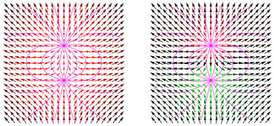
Figure 1.
Schematic diagrams depicting the imaginary part of the Q-field of two opposite unit charges by arrows. The lines represent some electric flux lines. We observe that they coincide with the lines of a constant -field. The configurations are rotational-symmetric about the axis through the two charge centres. In the red/green arrows, we encrypt also the positive/negative values of . For , the arrows are getting darker or black. The left configuration belongs to the topological quantum numbers and the right one to , where S is the total spin quantum number of the configuration. The numerical calculations are presented for the case of the spin singlet.
From the analytical calculations in Ref. [19], we know that MTP observes the inhomogeneous Maxwell equations. Therefore, we expect the classical Coulombic behaviour for point-like charges at large distances d between the charges of the dipole. After adjusting the asymptotic energies, this means
In Figure 2, we compare to the numerical results for the energy ; see Equation (A9), of the dipole in the spin singlet state. The diagram on the left shows the comparison in the range in steps for fm. For large distances d compared to the soliton radius parameter , the magnitude of the Coulomb attraction can be determined relatively easily. However, deviations from Coulombic behaviour, as shown in the right-hand diagram of Figure 2, are tiny and require high-precision calculations. There is no data for distances smaller than , as the soliton pair cannot be stabilised simply by fixing the soliton field to at the positions of the soliton centres.
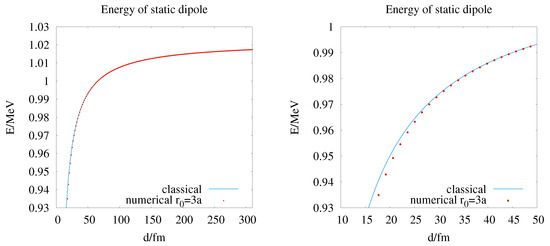
Figure 2.
Comparison between the classical Coulomb potential and the numerical values of the energy according to Equation (A9) of a static electron–positron pair as a function of the distance d between the two charges. Due to the finite size of solitons, we observe deviations of the energy of the static dipole (red circles) from the classical value for point sources (full blue line).
We describe these small deviations by a d-dependence of the fine structure constant
In Figure 3, we can easily observe whether the asymptotic energy is well chosen, as tiny variations in destroy the asymptotic behaviour of at large d. The running of the coupling already determined in Figure 2 can be clearly seen in Figure 3 below distances of 50 fm.
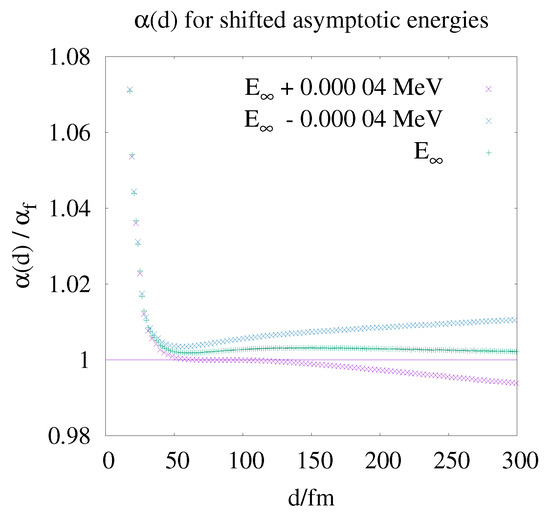
Figure 3.
Influence of the choice of on the asymptotic behaviour of according to Equation (17). Note that tiny variations in lead to incorrect asymptotic behaviour for large charge separations.
To be able to reach smaller values of d before the attraction becomes too strong and the dipole collapses, Ref. [21] suggested minimizing the energy functional of Equation (A10), which suppresses photonic excitations. In the calculations, see Figure 4; it turns out that it helps to approach shorter distances, but at distances of about 30 fm it can lead to an unphysical stiffness of the fields and to a strong reduction in .
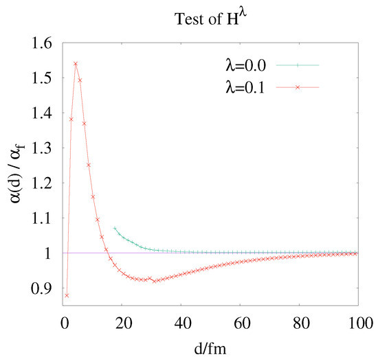
Figure 4.
The suppression of photonic excitations by the -dependent term in Equation (A10) allows shorter distances to be approached, but leads to an unphysical reduction of by distances of 30 fm, as can be clearly observed for .
This unphysical behavior can be observed from . On closer inspection of Figure 3, we see a similar but very tiny additional stiffness also in the results. It is not yet clear whether the minimum of at fm is a physical effect or an error of approximation, e.g., of the boundary conditions. Due to its small size, this effect is not really visible in Figure 4 at .
For tiny , we can move on to smaller distances d. The corresponding data are plotted in Figure 5. With the careful and elaborate determination of the interaction potential described above, we observe a nice Coulombic behaviour with constant coupling strength at distances above 50 fm and a strong increase in the effective charge at distances below 40 fm. This is the first observation of a running of the charge at the classical level in a purely Coulombic system.
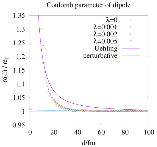
Figure 5.
The increase in at short distance d of the monopole pair is clearly visible in the data points for different values. These numerical results are compared with the analytical formulae of first-order perturbation theory (18) in QED and its long-range approximation (19). The strong attraction at short distances d does not allow the positions of the charges to be stabilised by fixing the centres of the solitons with the energy functional (A9). For shorter distances, the functional of the Equation (A10) can be used for the minimisation procedure. For small values of , the potential is only weakly distorted.
The only physical effect reasonable to be compared with is the rise in the coupling in perturbative QED as described in Ref. [22]. For comparison, we show the prediction of first-order perturbation theory and its long-distance approximation, which is well known as Uehling potential.
In QED, the interaction between charges is described by photon exchange. The algebraic form of the photon propagator therefore determines the strength of the interaction. The perturbation corrections for the photon propagator on the tree level are divergent. Even the first-order contribution, which is shown by the electron loop diagram in Figure 6, is divergent and requires regularisation and renormalisation.
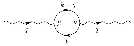
Figure 6.
Electron loop diagram as a contribution to the photon propagator at four-momentum q in first-order perturbation theory.
A perfect regularisation method is dimensional regularisation. Its success results from the preservation of symmetries, except for scale invariance. In the renormalisation process, an infinite photon self-energy is subtracted. It is set in such a way that the divergence of the photon propagator is cancelled. The invariance under a change in the finite terms subtracted in this process requires a change in the electric charge at large momentum transfers and small distances. This is usually interpreted as a change in photon structure due to virtual electron–positron pairs. This prediction of perturbation theory leads to a radially dependent fine structure constant
where is the reduced Compton wavelength of the electrons and is the relativistic factor for the mass of a moving particle. The correction can be determined by numerical integration and leads to the “perturbative‘’ curve in Figure 5. The approximation for large is [22]
For comparison, it is shown in Figure 5 as an approximation to the “Uehling” potential. This large-distance approximation reflects the numerical results of running the charge in the expected order of magnitude.
5. Conclusions
In the model of topological particles, we can describe electric or magnetic monopoles and their interaction without divergences. If we compare the finite masses of the stable soliton states with the electron mass, the finite size of the solitons is of the same order of magnitude as the classical electron radius. Since analytical solutions of this model are only known for one-particle systems, we have to analyse the interacting systems of two monopoles numerically with high precision. In this first calculation, we analyse the classical monopole–antimonopole potential in the spin-zero state. For large distances d between the charges, the potential has a pure behaviour. For the first time, we observe the running of the charge at the classical level in a purely Coulombic system, a running that can be explained by the geometric size of the solitons. It is a natural question how this running compares with the running of the coupling in QED. As an important result of the calculations, we would like to emphasise that the increase in the coupling occurs at the same length scale as predicted by the long-distance approximation of perturbative QED; see Figure 5.
In further calculations, the accuracy of the calculation should be increased through the use of adaptive lattices. This would make it possible to reduce the influence of boundary effects. As these first numerical calculations were carried out in the static limit, major changes can be expected for more realistic dynamic scenarios. It would be particularly interesting to insert the potential resulting from such a more detailed calculation into the Schrödinger and Dirac equation [23]. This would lead to shifts in the Dirac energy levels that could be compared with the Lamb shift. Further calculations should be performed for the spin-one state and for the repulsive system with two equal charges, where the cylindrical symmetry is lost.
The comparison with QED leads to important conclusions. The dynamical term of the Lagrangian (2) differs little from the term of electrodynamics. The difference between the two descriptions lies in the non-Abelian nature of the field and the potential term , which had to be introduced to stabilize solitons as extended particles in a field and replaces the fermionic part of the Lagrangian of QED. Solitons are in this sense a bosonized version of massive spin-1/2 fermions, similar to the Sine–Gordon solitons [24] being a bosonized version of the Thirring model fermions. Further interesting conclusions can be drawn from the potential term. For electrons, it is a quarter of the mass and contributes with this amount to the energy density in the universe. It has the form of a cosmological function , which could result in Einstein’s cosmological constant as an average value. If this ratio is also assumed for nucleons, an average density of 14.5 nucleons per m3 is needed to explain the average energy density in the universe. In their results from 2018, the Planck Collaboration [25] gives an average energy density of 0.69 , whereby the critical energy density is . Due to the large number of quantum fluctuations, the standard model cannot really explain this value. All predictions are very many orders of magnitude too large or zero. This is known as the “cosmological constant problem”.
The potential term could also be the basis of a cosmic inflation mechanism. According to Equation (2), the transition from a state to a state with releases an energy density of . In addition, the potential term leads to a non-vanishing trace of the energy–momentum tensor
Since its canonical form is already symmetrical, it correctly reflects the internal stresses. In QFT, one speaks of an anomaly if a symmetry that is present in classical theory is violated in quantum theory. In classical Maxwell–Dirac electrodynamics, in the tree approximation of QED, a scale transformation results in the trace of the energy–momentum tensor, as explained in Section 19.5 of Ref. [22]. This trace vanishes if the electrons have no (bare) mass. In the quantum description of QED, however, the trace does not vanish for massless electrons, which is referred to as a “trace anomaly”. Ref. [22] comments on this on page 686: “...the trace anomaly can be found in many different ways. For each possible method of regulating a quantum field theory, there is a derivation of the trace anomaly that exploits the possible pathology of that particular regulator.” and “...each derivation of the anomaly with a different regulator, taken individually, seems artificial, as if there were a problem with the field theory that we are not quite clever enough to fix. Eventually, though, we are forced to conclude that the quantum field theory is trying to tell us something”.
If we insert the Lagrangian (2) into the expression for the trace of the energy–momentum tensor (20), we immediately see that the terms in the trace that depend on the curvature tensor and thus on the electric and magnetic field strengths cancel each other out. What remains is the quadruple of the potential energy,
i.e., an expression that is composed only of the consistently positive (non-negative) contributions of the potential energy densities of the solitons. The potential term in the Lagrangian (2), which was introduced to stabilize solitons, obviously violates the scale invariance explicitly. Therefore, already in this classical description, the trace of the energy–momentum tensor has the same behavior as the quantum version of electrodynamics, QED, and thus provides an indication of the answer to the question in Ref. [22]. The quantum formulation could indicate the necessity of a potential term in the classical formulation. Instead of the anomaly, there would be explicit symmetry breaking.
Author Contributions
Conceptualization, M.F.; software, J.W., J.R., D.T. and F.A.; data curation, D.T.; visualization, F.A.; writing original draft preparation, F.A. and M.F.; writing review and editing, F.A. and M.F. All authors have read and agreed to the published version of the manuscript.
Funding
This research received no external funding.
Data Availability Statement
The original contributions presented in this study are included in the article. Further inquiries can be directed to the corresponding author.
Acknowledgments
The authors acknowledge TU Wien for its financial support through its Open Access Funding Programme.
Conflicts of Interest
The authors declare no conflicts of interest.
Appendix A. Dipoles on a Cylindrical Lattice
According to the Lagrangian (2) there are two contributions to the energy density of a static dipole,
the electric part of the curvature energy and the potential energy. A detailed derivation of these energy contributions of the field in cylindrical coordinates was given in [21]. The curvature energy in these coordinates is
Due to the cylindrical symmetry of the field configurations in Figure 1, it is sufficient to restrict the numerical integrations to a lattice in the -plane; see Figure A1. Inside the lattice, we minimise the energy according to the numerical formulation of the MTP Lagrangian. Outside the lattice, we use Maxwell’s electrodynamics [6] to calculate the energy. The numerical calculations of dipole field configurations were based on the algorithms discussed in [26,27,28] and their accuracy was tested in [21] by applying them to the analytically solvable monopole configuration. The coordinates in radial and z-direction are denoted by and , respectively. The radius of a soliton, , determines the length scale and thus the lattice spacing,
A numerical gradient minimisation algorithm is used to find the dipole configurations that minimise the total energy according to Equation (A1) for a given distance between the opposite charges.
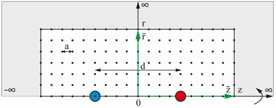
Figure A1.
Two solitons with opposite charges are separated by a distance d on a discrete lattice in the plane . The total number of points is and the lattice constant in both directions is a.
A good estimate of the initial configuration helps to reduce the runtime of the calculation. We obtain the real part of the initial Q-field from the profile function of a single monopole,
The modulus of the vector part of the Q-field is
We obtain a suitable initial direction of the field from the coincidence between electric field lines and lines of the constant field, which we observe in Figure 1. The field lines are defined by the differential equation,
with
After solving the differential Equation (A6), an analytical expression is found for the initial polar angle of the field,
So far, only points on the lattice have been included in the energy calculation. Outside the lattice, we use Maxwell’s electrodynamics to account for the curvature energy. The error due to neglecting the potential and tangential energy components outside the lattice is shown to be tiny (<0.2%) for a single monopole when the distance between the soliton core and the lattice boundaries is larger than [21]. Therefore, we find the energy outside the lattice by , which is numerically integrated using a trapezoidal summation, where the electric field strength is given by Equation (A7).
The principle of energy minimisation is used to find the dipole field configuration and the associated energy. The minimisation algorithm is adopted from https://de.mathworks.com/matlabcentral/fileexchange/75546-conjugate-gradient-minimisation, accessed on 1 June 2020. It is a multidimensional conjugate gradient method to find a local minimum of an energy functional that depends on the Q-field components at each lattice point, with ,
where is the lattice version of of Equation (A1).
However, if the centre of the solitons is only fixed for small dipole distances d, the annihilation of the two solitons is observed. To suppress this behaviour, it was proposed in Ref. [21] to smooth the soliton field by adding to the energy functional the term
in the minimisation process, where . During the calculations, it turned out that this additional term tends to suppress the interaction between the solitons. Therefore, we could only use tiny values of . This was sufficient to approach smaller distances.
The parameters used for the minimisation process are listed in Table A1.
Table A1.
Input parameters for the energy minimisation algorithm.
Table A1.
Input parameters for the energy minimisation algorithm.
| Parameter | Description | Used Value |
|---|---|---|
| Max. number of iterations | 5000 | |
| Min. gradient difference for two consecutive iterations | 1 | |
| Min. energy difference for two consecutive iterations | 1 | |
| Lower bound on the step size of the norm of the Q field | 1 |
We set the lattice spacing to fm. This a is small enough to obtain a reasonable approximation of the rest energy of the electrons.
It is not possible to use periodic boundary conditions for a dipole. When minimising the energy, we fix the soliton field Q at the edge of the lattice according to the initial configuration discussed after Equation (A4). This implies the assumption outside the lattice and leads to a small error in the potential energy, which is difficult to avoid.
Nevertheless, the boundary conditions have a major influence on the numerical results. With fixed lattice sizes and varying size d of the dipole, we are not able to achieve large d values due to boundary effects. It turns out that it is much better to increase the lattice size with increasing d while keeping the distance to the boundary constant. The lattice sizes we use for our calculations are 45 lattice spacings larger in the r and z directions than the relative distance d between the charges. We use and and all even distances .
Due to the finite size of the lattice, there remains a deviation of the asymptotic energy of the dipole from the mass of two non-interacting solitons, MeV. Since we fix the centres of the solitons at lattice sites, we obtain a weak even–odd effect for the lattice sizes for . For the asymptotic values of the calculated energies, we obtain MeV for even and MeV for odd r.
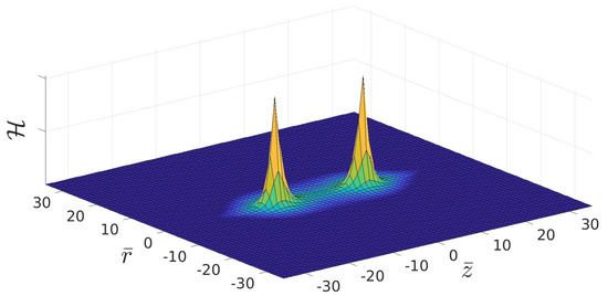
For the distance , we show some results of the minimisation process for the spin singlet configuration. In Figure A2, we compare the -field in the initial and final configuration in a restricted region. In particular, the minimisation changes the field in the region between the charges. The final values of the real part of the soliton field are shown in Figure A3. We note that the distribution of the values appears to be much broader than the distribution of the energy density in Figure A4 with very pronounced peaks reflecting the finite self-energy of charges according to Equation (A1).
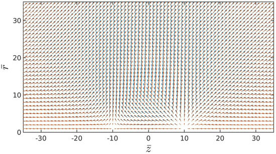
Figure A2.
The change in the imaginary part of the soliton field is shown by arrows. The initial configuration is shown in blue and the result of the minimisation process in red. Only a partial area of the lattice is shown. Due to the finite size of the solitons, , the centres of the charges approach the length of the arrows, as described by Equation (8).
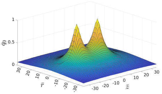
Figure A3.
distribution after minimisation for the configuration of Figure A2.
References
- Faber, M. A model for topological fermions. Few Body Syst. 2001, 30, 149–186. [Google Scholar] [CrossRef]
- Faber, M. A Geometric Model in 3+1D Space-Time for Electrodynamic Phenomena. Universe 2022, 8, 73. [Google Scholar] [CrossRef]
- Dirac, P.A.M. Quantised singularities in the electromagnetic field. Proc. R. Soc. Lond. 1931, A133, 60–72. [Google Scholar]
- Dirac, P.A.M. The Theory of magnetic poles. Phys. Rev. 1948, 74, 817–830. [Google Scholar]
- Millikan, R.A. On the Elementary Electrical Charge and the Avogadro Constant. Phys. Rev. 1913, 2, 109–143. [Google Scholar] [CrossRef]
- Jackson, J. Classical Electrodynamics; Wiley: Hoboken, NJ, USA, 1999. [Google Scholar]
- Wu, T.T.; Yang, C.N. Concept of nonintegrable phase factors and global formulation of gauge fields. Phys. Rev. D 1975, 12, 3845–3857. [Google Scholar] [CrossRef]
- Wu, T.T.; Yang, C.N. Some Solutions of the Classical Isotopic Gauge Field Equations. In Properties of Matter Under Unusual Conditions; Mark, H., Fernbach, S., Eds.; John Wiley & Sons, Inc.: New York, NY, USA, 1969; pp. 349–354. [Google Scholar]
- Wu, T.T.; Yang, C.N. Some remarks about unquantized non-Abelian gauge fields. Phys. Rev. D 1975, 12, 3843–3844. [Google Scholar] [CrossRef]
- Georgi, H.; Glashow, S.L. Unified weak and electromagnetic interactions without neutral currents. Phys. Rev. Lett. 1972, 28, 1494. [Google Scholar] [CrossRef]
- ’t Hooft, G. Magnetic Monopoles in Unified Gauge Theories. Nucl. Phys. 1974, B79, 276–284. [Google Scholar] [CrossRef]
- Polyakov, A.M. Particle spectrum in quantum field theory. JETP Lett. 1974, 20, 194–195. [Google Scholar]
- Remoissenet, M. Waves Called Solitons: Concepts and Experiments/M. Remoissenet; Springer: Berlin, Germany, 1999. [Google Scholar]
- Skyrme, T.H.R. A Nonlinear theory of strong interactions. Proc. R. Soc. Lond. A 1958, 247, 260–278. [Google Scholar] [CrossRef]
- Skyrme, T.H.R. A Nonlinear field theory. Proc. R. Soc. Lond. A 1961, 260, 127–138. [Google Scholar] [CrossRef]
- Skyrme, T.H.R. A Unified Field Theory of Mesons and Baryons. Nucl. Phys. 1962, 31, 556–569. [Google Scholar] [CrossRef]
- Makhankov, V.G.; Rybakov, Y.P.; Sanyuk, V.I. The Skyrme Model; Springer Series in Nuclear and Particle Physics; Springer: Berlin/Heidelberg, Germany, 1993; p. 265. [Google Scholar] [CrossRef]
- Adam, C.; Wereszczynski, A. Topological energy bounds in generalized Skyrme models. Phys. Rev. D 2014, 89, 065010. [Google Scholar] [CrossRef]
- Faber, M.; Kobushkin, A.P. Electrodynamic limit in a model for charged solitons. Phys. Rev. 2004, D69, 116002. [Google Scholar] [CrossRef]
- Schwinger, J. Electromagnetic mass revisited. Found. Phys. 1983, 13, 373–383. [Google Scholar] [CrossRef]
- Anmasser Fabian, T.D.; Manfried, F. About the Solution of the Numerical Instability for Topological Solitons with Long Range Interaction. Few-Body Syst. 2021, 62, 84. [Google Scholar]
- Peskin, M.E.; Schroeder, D.V. An Introduction to Quantum Field Theory, 1st ed.; Perseus Books Publishing, LLC.: New York, NY, USA, 1995; p. 842. [Google Scholar]
- Faber, M. From Soft Dirac Monopoles to the Dirac Equation. Universe 2022, 8, 387. [Google Scholar] [CrossRef]
- Gómez Nicola, A.; Steer, D. Thermal bosonisation in the sine-Gordon and massive Thirring models. Nucl. Phys. B 1999, 549, 409–449. [Google Scholar] [CrossRef]
- Aghanim, N.; Akrami, Y.; Arroja, F.; Ashdown, M.; Aumont, J.; Baccigalupi, C.; Ballardini, M.; Banday, A.J.; Barreiro, R.B.; Bartolo, N.; et al. Planck2018 results. Astron. Astrophys. 2020, 641, A1. [Google Scholar] [CrossRef]
- Wabnig, J. Interaction in the Model of Topological Fermions. Diploma Thesis, Technische Universität Wien, Vienna, Austria, 2001. [Google Scholar]
- Theuerkauf, D. Charged Particles in the Model of Topological Fermions. Diploma Thesis, Technische Universität Wien, Vienna, Austria, 2016. [Google Scholar]
- Anmasser, F. Running Coupling Constant in the Model of Topological Fermions. Diploma Thesis, Technische Universität Wien, Vienna, Austria, 2021. [Google Scholar]
Disclaimer/Publisher’s Note: The statements, opinions and data contained in all publications are solely those of the individual author(s) and contributor(s) and not of MDPI and/or the editor(s). MDPI and/or the editor(s) disclaim responsibility for any injury to people or property resulting from any ideas, methods, instructions or products referred to in the content. |
© 2025 by the authors. Licensee MDPI, Basel, Switzerland. This article is an open access article distributed under the terms and conditions of the Creative Commons Attribution (CC BY) license (https://creativecommons.org/licenses/by/4.0/).