Scaling Behavior and Phases of Nonlinear Sigma Model on Real Stiefel Manifolds Near Two Dimensions

Abstract

For a quasi-two-dimensional nonlinear sigma model on the real Stiefel manifolds with a generalized (anisotropic) metric, the equations of a two-charge renormalization group (RG) for the homothety and anisotropy of the metric as effective couplings are obtained in a one-loop approximation. Normal coordinates and the curvature tensor are exploited for the renormalization of the metric. The RG trajectories are investigated and the presence of a fixed point common to four critical lines or four phases (tetracritical point) in the general case, or its absence in the case of an Abelian structure group, is established. For the tetracritical point, the critical exponents are evaluated and compared with those known earlier for a simpler particular case.

1. Introduction

The nonlinear sigma model (NLSM), first introduced in [1] for a description of pion properties, has found generalizations which have become a very efficient tool in exploring diverse phenomena in quantum physics, including, e.g., magnetic systems [2,3,4] as well as the conductivity of disordered systems [5]. Soon after [1], the importance of using (differential) geometric methods in the construction and study of general phenomenological Lagrangians (NLSMs) was recognized (see [6,7,8]). Moreover, the importance of symmetric homogeneous (or coset) spaces was emphasized in [8] as well as in [5,9]. On the other hand, a few works [10,11,12] paid some attention to the potential role of nonsymmetric coset spaces as target spaces for the respective nonlinear sigma models.

Closely related to the well-known real Grassmann manifolds ${\mathrm{Gr}}_k\left({\mathbb{R}}^N\right)$ are their well-known extensions [13], such as the real Stiefel manifolds $V_k\left({\mathbb{R}}^N\right)$. The latter are nothing but principal fiber bundles with a base being the Grassmannian ${\mathrm{Gr}}_k\left({\mathbb{R}}^N\right)$ and the structure group $SO\left(k\right)$. We are interested in (quasi) two-dimensional sigma models—nonlinear field models with values in the Stiefel (or, in particular, Grassmann) manifolds. We note that the quantum properties of Grassmannian sigma models are quite well studied: in the two-dimensional case, such nonlinear models are characterized by asymptotic freedom [2,14], and if we extend to the dimension $d=2+\epsilon$, the models have a two-phase structure with a bicritical point [15]. This behavior, together with the use of the replica method and replica limit, allowed the description (see, e.g., [5]) of the (de)localization of electrons in disordered systems (or random potential) [16]. As for the classical two-dimensional Grassmannian models, their integrability was proven for these nonlinear field models [17].

Nonlinear sigma models on real Stiefel manifolds have radically different properties, both in the classical and especially quantum consideration [11,18], both for $d=2$ and $d=2+\epsilon$. In particular, in contrast to the single-charge RG (scaling) behavior of Grassmannian sigma models, the class of $V_k\left({\mathbb{R}}^N\right)$ sigma models is characterized by a two-charge behavior, and the question of the presence of asymptotic freedom in them at $d=2$ becomes quite nontrivial [11,18].

The extension of the ${\mathrm{Gr}}_k\left({\mathbb{R}}^N\right)$ sigma model to the $d=(2+\epsilon )$-dimensional nonlinear $V_k\left({\mathbb{R}}^N\right)$-model (of the fields defined on real Stiefel manifolds) is also very desirable in view of the following important reasons. First, since Grassmannians are Einstein manifolds, the single (effective) charge or coupling in the associated quantum sigma model is of pure geometrical origin—it is the homothety of metrics, i.e., uniform (or isotropic) scaling of a fixed metric. On the contrary, in the extended models on the spaces $V_k\left({\mathbb{R}}^N\right)$ the latter in general are not Einstein manifolds, and we come inevitably to the enriched set of couplings: besides homothety, a certain anisotropy of metrics comes into play. Then, the Einsteinian property may occur only very randomly (for one or two special values of the anisotropy). Second, because of such nontrivial geometry of $V_k\left({\mathbb{R}}^N\right)$, the related nonlinear sigma models in $d=2+\epsilon$ do manifest more complicated critical behavior: besides/instead of bicritical point, a tetracritical point may also appear. The third property is very important from the viewpoint of possible physical applications. Namely, we have in mind applying $V_k\left({\mathbb{R}}^N\right)$ sigma models to a more complex situation when the system manifesting (de)localization of electrons may also participate in superconductivity. It is clear that the involvement of an additional order parameter could then be related to the presence of a second coupling in the Stiefel model. Finally, the electron-hole symmetry that finds its natural reflection in the $k\leftrightarrow N-k$ symmetry of Grassmannian sigma models (see, e.g., [15]) is known to be inevitably broken within the superconductivity context as noted, e.g., in [19,20]. However, just the absence of $k\leftrightarrow N-k$ symmetry is an intrinsic feature of the Stiefel $V_k\left({\mathbb{R}}^N\right)$ sigma models.

Because of this, and also in connection with the recent return of interest [21,22] to the geometry and other properties of Stiefel manifolds, we will focus on the special properties of the nonlinear sigma model in $d=2+\epsilon$ Euclidean dimensions with the action functional $\mathcal{A}$ and the Lagrangian $\mathcal{L}$:

$$\mathcal{A}\left[U\right]={\displaystyle \frac{1}{2T}}\int \mathcal{L}{\mathrm{d}}^{d}x,\mathcal{L}\left[U\right]=\mathrm{Tr}\left[\nabla U^{\top }\nabla U+(\lambda -1)\nabla U^{\top }U{U}^{\top }\nabla U\right],$$

(1)

where we have introduced the temperature T, field $U\left(x\right)$ valued in the Stiefel manifold $V_k\left({\mathbb{R}}^N\right)=SO\left(N\right)/SO(N-k)$, gradient $\nabla =(\partial /\partial x_1,...,\partial /\partial x_d)$, and parameter (of the metric anisotropy) $\lambda >0$.

2. Some Characteristics of Stiefel Manifold

A real Stiefel manifold $V_k\left({\mathbb{R}}^N\right)$ is the set of all k-frames formed by sets of orthonormal vectors in the space ${\mathbb{R}}^N$. Any element $U\in V_k\left({\mathbb{R}}^N\right)$, given by an $N\times k$-matrix, satisfies the orthogonality condition $U^{\top }U=I_k$, where $I_k$ is the identity $k\times k$-matrix and ⊤ denotes the transpose. On such manifolds, the group $SO\left(N\right)$ acts transitively as the isometry group. The isotropy group corresponding to the “origin” $\mathcal{O}=\{{\mathbf{e}}_1,{\mathbf{e}}_2,...,{\mathbf{e}}_k\}$ consists of matrices of the form $\mathrm{diag}(I_k,H)$, where $H\in SO(N-k)$. This allows us to identify the manifold $V_k\left({\mathbb{R}}^N\right)$ with the quotient space $SO\left(N\right)/SO(N-k)$ with $\dim V_k\left({\mathbb{R}}^N\right)=Nk-k(k+1)/2$. Thus, $V_k\left({\mathbb{R}}^N\right)$ is defined as a submanifold of the space ${\mathbb{R}}^{N\times k}$. In particular, $V_1\left(\mathbb{R}\right)=\{1,-1\}$; $V_1\left({\mathbb{R}}^N\right)=S^{N-1}$ is an $(N-1)$-dimensional sphere; $V_N\left({\mathbb{R}}^N\right)=O\left(N\right)$; $V_{N-1}\left({\mathbb{R}}^N\right)=SO\left(N\right)$; and $V_2\left({\mathbb{R}}^4\right)$ is the first nontrivial case.

Tangent space. Let $\mathcal{TM}$ be the tangent space for $\mathcal{M}=V_k\left({\mathbb{R}}^N\right)$. We require that each tangent vector $\xi \in {\mathcal{T}}_U\mathcal{M}$ at a point $U\in \mathcal{M}$ belongs to the horizontal subspace, i.e., it has the following structure [21,22,23]:

$$\begin{array}{ccc}& & \xi =U{\omega }_{\xi }+F_{\xi },\hfill \\ & & {\omega }_{\xi }={\displaystyle \frac{1}{2}}(U^{\top }\xi -{\xi }^{\top }U)\in \mathfrak{o}\left(k\right),F_{\xi }=\mathrm{\Pi }\xi ,\hfill \end{array}$$

(2)

where the projector $\mathrm{\Pi }=I_N-U{U}^{\top }$, and ${\omega }_{\xi }^{\top }=-{\omega }_{\xi }$. Since ${\omega }_{\xi }$ consists of $k(k-1)/2$ independent matrix components and $F_{\xi }$ contains $(N-k)k$ components, their total sum restores $\dim V_k\left({\mathbb{R}}^N\right)$. Conversely, the symmetric component $(U^{\top }\xi +{\xi }^{\top }U)/2$ belongs to the vertical subspace.

Tangent vectors can be defined in the respective Lie algebra $\mathfrak{so}\left(N\right)$, the basis of which is formed by $N(N-1)/2$ skew-symmetric $N\times N$-matrices $X_A$:

$$X_A=∥{\left(X_A\right)}_{b,c}∥=∥{\delta }_{b,a_1}{\delta }_{c,a_2}-{\delta }_{b,a_2}{\delta }_{c,a_1}∥,$$

(3)

where the multi-index $A=(a_1,a_2)$ consists of the two subsets such that $1\le a_1,a_2\le N$. The matrix $X_A$ has only two nonzero elements, 1 and $-1$, at positions $(a_1,a_2)$ and $(a_2,a_1)$, so that $X_A^{\top }=-X_A$ and $\mathrm{Tr}\left(X_A^{\top }{X}_A\right)=2$. The basis elements of the algebra $\mathfrak{so}\left(N\right)$ satisfy the commutation relations:

$$\begin{array}{ccc}& [X_A,X_B]=f_{AB}^C{X}_C,& \hfill \\ & f_{AB}^C={\delta }_{a_1,b_1}{\delta }_{a_2}^{c_1}{\delta }_{b_2}^{c_2}+{\delta }_{a_2,b_2}{\delta }_{a_1}^{c_1}{\delta }_{b_1}^{c_2}-{\delta }_{a_2,b_1}{\delta }_{a_1}^{c_1}{\delta }_{b_2}^{c_2}-{\delta }_{a_1,b_2}{\delta }_{a_2}^{c_1}{\delta }_{b_1}^{c_2}.& \hfill \end{array}$$

(4)

In this basis, the orthonormal metric $g(X,Y)=-\mathcal{B}(X,Y)/\left[2\right(N-2\left)\right]$ based on the bi-invariant Killing form $\mathcal{B}(X,Y)$, when $\mathcal{B}(X_A,X_B)=f_{AC}^D{f}_{BD}^C$, coincides with the Frobenius metric, which is natural in the description of the $\sigma$-model (1):

$${\langle X_A,X_B\rangle }_F={\displaystyle \frac{1}{2}}\mathrm{Tr}\left(X_A^{\top }{X}_B\right)={\delta }_{AB}.$$

(5)

Then, the norm of the vector $\xi \in \mathcal{TM}$ is written as ${\parallel \xi \parallel }_F^2=(1/2)\mathrm{Tr}\left({\xi }^{\top }\xi \right)$.

To write the $\omega$- and F-components of tangent vectors in the basis introduced, we define $X_P$ and $X_Q$ with $P=(p,q)$ and $Q=(j,p)$, where $1\le p,q\le k$ and $k+1\le j\le N$. Although $F\in {\mathbb{R}}^{N\times k}$ in (2), it has $(N-k)k$ independent components and is usually included in meaningful expressions as a combination $F^{\top }F$.

Metric. The covariant metric $\mathrm{g}(U;\lambda )$ (metric operator) of model (1) and its action on the tangent vector $\xi \in {\mathcal{T}}_U\mathcal{M}$ are defined as

$$\mathrm{g}\xi =\xi +(\lambda -1)U{U}^{\top }\xi ,{\mathrm{g}}^{-1}\xi =\xi +({\lambda }^{-1}-1)U{U}^{\top }\xi ,\det \mathrm{g}={\lambda }^k.$$

(6)

Note that the case $\lambda =1/2$ is called canonical in the literature [22,23].

Then the inner (scalar) product of two tangent vectors $\xi ,\eta \in {\mathcal{T}}_U\mathcal{M}$ is given as

$${\langle \xi ,\eta \rangle }_{\mathrm{g}}=\mathrm{Tr}\left[{\xi }^{\top }\eta +(\lambda -1){\xi }^{\top }U{U}^{\top }\eta \right].$$

(7)

Since ${\langle \xi ,\xi \rangle }_{\mathrm{g}}=\mathrm{Tr}(\lambda {\omega }_{\xi }^{\top }{\omega }_{\xi }+F_{\xi }^{\top }{F}_{\xi })$, according to (2), the Lagrangian in (1) becomes

$$\mathcal{L}=\mathrm{Tr}(\lambda {\omega }_u^{\top }{\omega }_u+{\mathbf{F}}_u^{\top }{\mathbf{F}}_u).$$

(8)

Here we use the following decomposition of the tangent vector $\nabla U$:

$$\begin{array}{ccc}& \nabla U=U{\omega }_u+{\mathbf{F}}_u,& \hfill \\ & {\omega }_u=U^{\top }\nabla U,{\mathbf{F}}_u=\mathrm{\Pi }\nabla U,& \hfill \end{array}$$

(9)

because $\nabla U^{\top }U+U^{\top }\nabla U=0$ due to the constraint $U^{\top }U=I_k$.

Expression (8) indicates the presence of two $\omega$- and F-subsystems. The condition $U^{\top }U=I_k$ can be easily satisfied by reducing the system to an $O\left(k\right)$-model with ${\omega }_u\ne 0$ and ${\mathbf{F}}_u=0$. If ${\omega }_u$ is expressed through ${\mathbf{F}}_u\ne 0$, then a model on the Grassmannian ${\mathrm{Gr}}_k\left({\mathbb{R}}^N\right)=SO\left(N\right)⁄[SO(N-k)\times SO\left(k\right)]$ is obtained. However, our focus here is on incorporating both subsystems, utilizing the full number of degrees of freedom, $\dim V_k\left({\mathbb{R}}^N\right)$.

Linear connection and normal coordinates. Consider the auxiliary problem of one-dimensional evolution, which is generated by the action functional:

$$S=\int \mathrm{d}t\left\{\mathrm{Tr}\left[{\dot{U}}^{\top }\dot{U}-(\lambda -1){\left(U^{\top }\dot{U}\right)}^2\right]+\mathrm{Tr}\left[H(U^{\top }U-I_k)\right]\right\},$$

(10)

where $H^{\top }=H\in {\mathbb{R}}^{k\times k}$ is a Lagrange multiplier; $\dot{U}=\mathrm{d}U/\mathrm{d}t$.

By varying $U\left(t\right)$ and H and using certain identities, one can obtain the multiplier $H=-{\dot{U}}^{\top }\dot{U}+2(\lambda -1){\left(U^{\top }\dot{U}\right)}^2$ and the equation of the geodesic [21]:

$$\ddot{U}+\mathrm{\Gamma }(\dot{U},\dot{U})=0.$$

(11)

To write the latter, we used the expression for the Christoffel function (symbol of the second kind), which defines the linear connection at the point $U\in \mathcal{M}$:

$$\mathrm{\Gamma }(\xi ,\eta )={\displaystyle \frac{1}{2}}U\left({\xi }^{\top }\eta +{\eta }^{\top }\xi \right)+(1-\lambda )\mathrm{\Pi }\left(\xi {\eta }^{\top }+\eta {\xi }^{\top }\right)U.$$

(12)

Now, we present the solution of Equation (11) as a series in t in terms of the initial data $U\left(0\right)=U_0$ and $\dot{U}\left(0\right)=V$, which are related by $U_0^{\top }V+V^{\top }{U}_0=0$. One has

$$U\left(t\right)=U_0+tV-{\displaystyle \frac{t^2}{2!}}{\mathrm{\Gamma }}_0(V,V)-{\displaystyle \frac{t^3}{3!}}{\mathrm{\Gamma }}_0(V,V,V)-\dots ,$$

(13)

where ${\mathrm{\Gamma }}_0(V,V)={\left.\mathrm{\Gamma }(V,V)\right|}_{U=U_0}$, and ${\mathrm{\Gamma }}_0(V,V,V)={\left.{\mathrm{D}}_V\mathrm{\Gamma }(V,V)-2\mathrm{\Gamma }(V,\mathrm{\Gamma }(V,V))\right|}_{U=U_0}$ involves the derivative ${\mathrm{D}}_V$ at the point $U\in \mathcal{M}$ in the direction $V\in \mathcal{TM}$, which acts, in particular, as

$$\begin{array}{ccc}\hfill {\mathrm{D}}_{\varphi }\mathrm{\Gamma }(\xi ,\eta )& =& {\displaystyle \frac{1}{2}}\varphi \left({\xi }^{\top }\eta +{\eta }^{\top }\xi \right)-(1-\lambda )\left(\varphi U^{\top }+U{\varphi }^{\top }\right)\left(\xi {\eta }^{\top }+\eta {\xi }^{\top }\right)U\hfill \\ & & +(1-\lambda )\mathrm{\Pi }\left(\xi {\eta }^{\top }+\eta {\xi }^{\top }\right)\varphi .\hfill \end{array}$$

(14)

Note that the expansions (2) and (9) can be applied after calculating such a derivative.

It is easy to verify in the approximation $t^2$ that $I_k=U^{\top }U=U_0^{\top }{U}_0$. Thus, setting $t=1$, the two points $U,U_0\in \mathcal{M}$ are related by (13). Restoring the dependence of U and V on the coordinates x, formula (13) generalizes the “field shift” $U=U_0+V$ in Euclidean space when $U,U_0,V\in {\mathbb{R}}^{\dim \mathcal{M}}$. Thus, fixing $U_0$, the variables V are called normal coordinates, which further describe quantum fluctuations in the $\sigma$-model.

Curvature. We define the curvature tensor $R(\xi ,\eta )\varphi$ in $(1,3)$-form for $\xi ,\eta ,\varphi \in \mathcal{TM}$ as (see [22])

$$R(\xi ,\eta )\varphi ={\mathrm{D}}_{\eta }\mathrm{\Gamma }(\xi ,\varphi )-{\mathrm{D}}_{\xi }\mathrm{\Gamma }(\eta ,\varphi )+\mathrm{\Gamma }(\eta ,\mathrm{\Gamma }(\xi ,\varphi ))-\mathrm{\Gamma }(\xi ,\mathrm{\Gamma }(\eta ,\varphi )).$$

(15)

Let us calculate the components of $R(\xi ,\eta )\xi =U\left(U^{\top }R(\xi ,\eta )\xi \right)+\mathrm{\Pi }R(\xi ,\eta )\xi$:

$$\begin{array}{cc}\hfill U^{\top }R(\xi ,\eta )\xi =& -{\displaystyle \frac{1}{4}}({\omega }_{\eta }{\omega }_{\xi }^2-2{\omega }_{\xi }{\omega }_{\eta }{\omega }_{\xi }+{\omega }_{\xi }^2{\omega }_{\eta })+{\displaystyle \frac{\lambda }{2}}({\omega }_{\eta }{F}_{\xi }^{\top }{F}_{\xi }+F_{\xi }^{\top }{F}_{\xi }{\omega }_{\eta })\hfill \\ & +{\displaystyle \frac{3-4\lambda }{4}}({\omega }_{\xi }{F}_{\xi }^{\top }{F}_{\eta }+F_{\eta }^{\top }{F}_{\xi }{\omega }_{\xi })-{\displaystyle \frac{3-2\lambda }{4}}({\omega }_{\xi }{F}_{\eta }^{\top }{F}_{\xi }+F_{\xi }^{\top }{F}_{\eta }{\omega }_{\xi }),\hfill \end{array}$$

(16)

$$\begin{array}{cc}\hfill \mathrm{\Pi }R(\xi ,\eta )\xi =& -\lambda {\displaystyle \frac{3-4\lambda }{2}}{F}_{\xi }{\omega }_{\xi }{\omega }_{\eta }+\lambda {\displaystyle \frac{3-2\lambda }{2}}{F}_{\xi }{\omega }_{\eta }{\omega }_{\xi }-{\lambda }^2{F}_{\eta }{\omega }_{\xi }^2+F_{\eta }{F}_{\xi }^{\top }{F}_{\xi }\hfill \\ & +{\displaystyle \frac{2-3\lambda }{2}}{F}_{\xi }{F}_{\xi }^{\top }{F}_{\eta }-{\displaystyle \frac{4-3\lambda }{2}}{F}_{\xi }{F}_{\eta }^{\top }{F}_{\xi }.\hfill \end{array}$$

(17)

The bi-quadratic form $\tilde{K}(\xi ,\eta )={\langle R(\xi ,\eta )\xi ,\eta \rangle }_{\mathrm{g}}$, which characterizes the sectional curvature [24], can be expressed, after substituting expressions (16) and (17), as follows:

$$\begin{array}{ccc}\hfill \tilde{K}(\xi ,\eta )& =& {\displaystyle \frac{\lambda }{2}}{∥[{\omega }_{\xi },{\omega }_{\eta }]∥}_F^2+{∥F_{\eta }{F}_{\xi }^{\top }-F_{\xi }{F}_{\eta }^{\top }∥}_F^2+{\displaystyle \frac{2-3\lambda }{2}}{∥F_{\eta }^{\top }{F}_{\xi }-F_{\xi }^{\top }{F}_{\eta }∥}_F^2\hfill \\ & & +2{\lambda }^2\left({∥F_{\eta }{\omega }_{\xi }∥}_F^2+{∥F_{\xi }{\omega }_{\eta }∥}_F^2\right)+2\lambda (3-4\lambda ){\langle F_{\xi }{\omega }_{\xi },F_{\eta }{\omega }_{\eta }\rangle }_F\hfill \\ & & -2\lambda (3-2\lambda ){\langle F_{\xi }{\omega }_{\eta },F_{\eta }{\omega }_{\xi }\rangle }_F.\hfill \end{array}$$

(18)

A similar formula is derived in the work ([25], p. 405) in terms of rectangular $(N-k)\times k$-matrices, say M, instead of $F\in {\mathbb{R}}^{N\times k}$. However, it does not matter, because M and F are entered as combinations $M^{\top }M$ and $F^{\top }F$, which both belong to ${\mathbb{R}}^{k\times k}$.

Using (16) and (17) and contracting the $(1,3)$-curvature (see Appendix A.1), the diagonal components of the Ricci $(0,2)$-tensor are obtained [22]:

$$\mathrm{Ric}(\xi ,\xi )=\left[{\lambda }^2(N-k)+{\displaystyle \frac{k-2}{4}}\right]\mathrm{Tr}\left({\omega }_{\xi }^{\top }{\omega }_{\xi }\right)+\left[N-2-\lambda (k-1)\right]\mathrm{Tr}\left(F_{\xi }^{\top }{F}_{\xi }\right).$$

(19)

It is seen that the curvature coefficients are constant due to the homogeneity of the Stiefel manifold (see [18]). We are discussing the relation between $\tilde{K}$ and $\mathrm{Ric}$ when renormalizing the $\sigma$-model.

3. Background Field Formalism

We assume that the Lagrangian $\mathcal{L}\left[U_0\right]=\mathrm{Tr}(\nabla U_0^{\top }{\mathrm{g}}_0\nabla U_0)$ is determined by the bare metric $\mathrm{g}=\mathrm{g}(U;\lambda )$, which differs from ${\mathrm{g}}_0=\mathrm{g}(U_0;\lambda )$ by the covariant counterterms $\mathrm{h}$:

$$\mathrm{g}={\mu }^{\epsilon }{\mathrm{g}}_0+\mathrm{h},$$

(20)

where $\epsilon =d-2$ is the renormalization parameter; $\mu$ is the renormalization scale.

This renormalization constitutes our primary concern, though the fields themselves are also subject to renormalization. To address this, we adapt a well-known procedure (see [26,27]) to the model defined on the Stiefel manifold. Initially, we present a covariant description utilizing normal coordinates.

Effective Lagrangian. Let us introduce the interpolating field $\mathrm{\Phi }(x,s)$ and quantities similar to those defined earlier:

$$\mathrm{\Phi }(x,0)=U_0\left(x\right),{\left.{\displaystyle \frac{\partial \mathrm{\Phi }(x,s)}{\partial s}}\right|}_{s=0}=V,\mathrm{\Phi }(x,1)=U\left(x\right).$$

(21)

Let us expand the Lagrangian $\mathcal{L}\left[U\right]$ in a series with respect to the parameter s:

$$\mathcal{L}\left[U\right]\equiv \mathcal{L}\left[\mathrm{\Phi }(x,1)\right]=\sum _{n=0}^{\infty }{\displaystyle \frac{1}{n!}}{\left.{\displaystyle \frac{{\partial }^n\mathcal{L}\left[\mathrm{\Phi }(x,s)\right]}{\partial s^n}}\right|}_{s=0},$$

(22)

using the covariant derivative ${\widehat{\nabla }}_s$ along the geodesic $\mathrm{\Phi }(x,s)$, as well as $\widehat{\nabla }$:

$${\widehat{\nabla }}_s\xi \equiv {\displaystyle \frac{\partial \xi }{\partial s}}+\mathrm{\Gamma }\left({\displaystyle \frac{\partial \mathrm{\Phi }(x,s)}{\partial s}},\xi \right),\widehat{\nabla }\xi \equiv \nabla \xi +\mathrm{\Gamma }\left(\nabla \mathrm{\Phi }(x,s),\xi \right),$$

(23)

where the Christoffel function $\mathrm{\Gamma }(\xi ,\eta )$ from (12) is taken at $U=\mathrm{\Phi }(x,s)$.

Applying the decomposition of tangent vectors into $\omega$- and F-components, we obtain

$$\begin{array}{ccc}\hfill {\displaystyle \frac{\partial \mathcal{L}\left[\mathrm{\Phi }\right(x,s\left)\right]}{\partial s}}& =& 2\mathrm{Tr}\left(\nabla {\mathrm{\Phi }}^{\top }\mathrm{g}\widehat{\nabla }{\displaystyle \frac{\partial \mathrm{\Phi }}{\partial s}}\right),\hfill \end{array}$$

(24)

$$\begin{array}{ccc}\hfill {\displaystyle \frac{1}{2}}{\displaystyle \frac{{\partial }^2\mathcal{L}\left[\mathrm{\Phi }(x,s)\right]}{\partial s^2}}& =& \mathrm{Tr}\left[{\left(\widehat{\nabla }{\displaystyle \frac{\partial \mathrm{\Phi }}{\partial s}}\right)}^{\top }\mathrm{g}\widehat{\nabla }{\displaystyle \frac{\partial \mathrm{\Phi }}{\partial s}}\right]+\mathrm{Tr}\left(\nabla {\mathrm{\Phi }}^{\top }\mathrm{g}\left[{\widehat{\nabla }}_s,\widehat{\nabla }\right]{\displaystyle \frac{\partial \mathrm{\Phi }}{\partial s}}\right),\hfill \end{array}$$

(25)

taking into account that

$$\begin{array}{cc}{\widehat{\nabla }}_s{\displaystyle \frac{\partial \mathrm{\Phi }(x,s)}{\partial s}}=\hfill & 0,\hfill \end{array}$$

(26)

$$\begin{array}{cc}{\widehat{\nabla }}_s\nabla \mathrm{\Phi }(x,s)=\hfill & \widehat{\nabla }{\displaystyle \frac{\partial \mathrm{\Phi }(x,s)}{\partial s}}\equiv \nabla {\displaystyle \frac{\partial \mathrm{\Phi }(x,s)}{\partial s}}+\mathrm{\Gamma }\left({\displaystyle \frac{\partial \mathrm{\Phi }(x,s)}{\partial s}},\nabla \mathrm{\Phi }(x,s)\right),\hfill \end{array}$$

(27)

$$\begin{array}{cc}\left[{\widehat{\nabla }}_s,\widehat{\nabla }\right]\xi =\hfill & R\left(\nabla \mathrm{\Phi }(x,s),{\displaystyle \frac{\partial \mathrm{\Phi }(x,s)}{\partial s}}\right)\xi ,\hfill \end{array}$$

(28)

where the curvature $R(\xi ,\eta )\varphi$ is given by (15).

In the one-loop approximation, we restrict ourselves to the Lagrangian quadratic in V:

$$\mathcal{L}\left[U\right]=\mathcal{L}\left[U_0\right]+2{\langle \nabla U_0,\widehat{\nabla }V\rangle }_{{\mathrm{g}}_0}+{\langle \widehat{\nabla }V,\widehat{\nabla }V\rangle }_{{\mathrm{g}}_0}+{\langle \nabla U_0,R(\nabla U_0,V)V\rangle }_{{\mathrm{g}}_0},$$

(29)

where $\widehat{\nabla }V=\nabla V+{\mathrm{\Gamma }}_0(V,\nabla U_0)$, and ${\langle \nabla U_0,R(\nabla U_0,V)V\rangle }_{{\mathrm{g}}_0}=-\tilde{K}(\nabla U_0,V)$ by definition. If $U_0\left(x\right)$ is a solution of the equation of motion, the term ${\langle \nabla U_0,\widehat{\nabla }V\rangle }_{{\mathrm{g}}_0}$ does not contribute to the action integral. Since expression (29) is general for $\sigma$-models within this approximation, we proceed to the next step, which is standard for such models.

We replace V by $\mathcal{V}$ to transform $\mathrm{Tr}(\nabla V^{\top }{\mathrm{g}}_0\nabla V)$ into $\mathrm{Tr}(\nabla {\mathcal{V}}^{\top }\nabla \mathcal{V})$. To do this, we set $V=\tilde{e}\mathcal{V}$, where $\tilde{e}=\mathrm{g}(U_0;{\lambda }^{-1/2})$. Then ${\tilde{e}}^2={\mathrm{g}}_0^{-1}$ and ${\tilde{e}}^{\top }{\mathrm{g}}_0\tilde{e}=I_N$, and the relation between the components of the tangent vectors V and $\mathcal{V}$ is given by

$$V=U_0{\omega }_V+F_V,\mathcal{V}=U_0{\omega }_{\mathcal{V}}+F_V,{\omega }_{\mathcal{V}}={\lambda }^{1/2}{\omega }_V.$$

(30)

After introducing ${\omega }_{\mathcal{V}}$ instead of ${\omega }_V$, the quadratic part of the Lagrangian with respect to V takes on the form

$$\begin{array}{ccc}& {\mathcal{L}}_{\mathrm{eff}}={\langle \widehat{\nabla }V,\widehat{\nabla }V\rangle }_{{\mathrm{g}}_0}-\tilde{K}(\nabla U_0,\tilde{e}\mathcal{V}),& \end{array}$$

(31)

$$\begin{array}{ccc}& {\langle \widehat{\nabla }V,\widehat{\nabla }V\rangle }_{{\mathrm{g}}_0}=\mathrm{Tr}\left(\nabla {\omega }_{\mathcal{V}}^{\top }\nabla {\omega }_{\mathcal{V}}+\nabla F_V^{\top }\nabla F_V\right)+{\mathcal{L}}_{\mathrm{int}},& \hfill \end{array}$$

(32)

where the first term in (32) corresponds to the free evolution of fluctuations and determines the Green’s functions. In this free Lagrangian, we retain only the $F_V^Q$ components of $F_V\in {\mathbb{R}}^{N\times k}$ as independent, since the $F_V^P$ components merely represent the interaction of $F_V^Q$ with $U_0$ (see Appendix B.1).

Quantization. In fact, quantization here means calculating the partition function and average values using the methods of quantum theory, when the imaginary Planck constant $-\mathrm{i}\hslash$ is replaced by the real temperature T. We consider $U_0\left(x\right)$ as the background field, and ${\omega }_{\mathcal{V}}$ and $F_V$ as fluctuating quantities. Simultaneously, the components of the metric $\mathrm{g}$, including the positive parameters T and $\lambda$ (see (1)), play the role of coupling constants. In physical applications of $\sigma$-models for describing Anderson localization, the temperature T is often associated with the conductivity coefficient, which undergoes renormalization. On the other hand, the parameter $\lambda$ (anisotropy) appears in the Lagrangian (8) as a running (scale-dependent) factor.

Quantizing, one should introduce a path integral over the rapidly varying fields ${\omega }_{\mathcal{V}}$ and $F_V$ (with a source), which is calculated as a series using Feynman diagrams. In the case under consideration, all expressions correspond to the one-loop approximation. As usual, when averaging expressions, Wick’s theorem for pairing fields of the same sort does work and allows us to limit ourselves to considering only even terms. In principle, the integral over the slowly varying component $U_0\left(x\right)$ also needs to be applied, since it is ambiguous. Some computational aspects of this procedure are outlined in Appendix B.1.

Let us define the Green’s functions of the fields:

$$\langle \langle {\omega }_{\mathcal{V}}^{P_1}\left(x\right){\omega }_{\mathcal{V}}^{P_2}\left(y\right)\rangle \rangle ={\pi }_{P_1{P}_2}\Delta (x-y),\langle \langle F_V^{Q_1}\left(x\right)F_V^{Q_2}\left(y\right)\rangle \rangle ={\delta }_{Q_1{Q}_2}\Delta (x-y),$$

(33)

where the brackets $\langle \langle ...\rangle \rangle$ denote the quantum average in the vacuum state; and the components of the matrix field $F_V$ with multi-indices $Q_n=(j_n,p_n)$, where $1\le p_n\le k$ and $k+1\le j_n\le N$ are chosen as independent. In addition, the symbol ${\delta }_{Q_1{Q}_2}={\delta }_{j_1,j_2}{\delta }_{p_1,p_2}$, and the symbol

$${\pi }_{P_1{P}_2}={\displaystyle \frac{1}{2}}\left({\delta }_{p_1,p_2}{\delta }_{q_1,q_2}-{\delta }_{p_1,q_2}{\delta }_{q_1,p_2}\right)$$

(34)

for multi-indices $P_n=(p_n,q_n)$, $1\le p_n,q_n\le k$, and their contraction gives the number of degrees of freedom. The spatially dependent component is defined by the expression

$$\Delta (x-y)=T\int {\displaystyle \frac{{\mathrm{e}}^{\mathrm{i}k·(x-y)}}{k^2}}{\displaystyle \frac{{\mathrm{d}}^{d}k}{{\left(2\pi \right)}^d}},$$

(35)

which results from (32) and (A27).

4. Beta Functions of Effective Couplings

Renormalization. Due to the form (35), when averaging local expressions of the model, the infrared (IR) divergences arise, which can be mitigated by introducing a regulator. Softening the expressions at the IR boundary by using the scale $\mu$ and denoting the area of the unit sphere in d dimensions as ${\mathrm{\Omega }}_{d-1}=2{\pi }^{d/2}/\mathrm{\Gamma }(d/2)$, when $\epsilon =d-2\to 0$, we have

$$\Delta \left(0\right)=T{\displaystyle \frac{{\mathrm{\Omega }}_{d-1}}{{\left(2\pi \right)}^d}}\underset{\mu }{\int }{k}^{d-3}\mathrm{d}k=-{\displaystyle \frac{T}{2\pi \epsilon }}-{\displaystyle \frac{T}{2\pi }}\ln \mu +O\left(\epsilon \right).$$

(36)

At once, ultraviolet (UV) divergences are eliminated in a standard way for $\sigma$-models [28].

Thus, the metric renormalization in the one-loop approximation is induced by the term [26,27,28]

$$\int \langle \langle \tilde{K}(\nabla U_0,\tilde{e}\mathcal{V})\rangle \rangle {\mathrm{d}}^{d}x=\int \mathrm{Ric}(\nabla U_0,\nabla U_0)\Delta \left(0\right){\mathrm{d}}^{d}x.$$

(37)

The idea of proving formula (37) is based on the equality of the quantum average of $\tilde{K}$ over the fields ${\omega }_{\mathcal{V}}$ and $F_V$ and the average over the basis matrices, when $\nabla U_0=U_0{\omega }_u+{\mathbf{F}}_u$ (see Appendix A.1). That is, due to the homogeneity of the Stiefel manifold, the calculations can be shifted to the “origin” $\mathcal{O}$, allowing the use of the basis (3). Then, we perform the substitution ${\omega }_{\mathcal{V}}^P\to X_P$, $F_V^Q\to \mathrm{\Pi }{X}_Q$, while the fields themselves are absorbed by $\Delta$. We also express $\nabla U_0$ in the basis (3) and sum over Q and the independent indices of P. When averaging $\tilde{K}(\nabla U_0,\tilde{e}\mathcal{V})$, only the terms quadratic in ${\omega }_{\mathcal{V}}$ and $F_V$ survive, and we obtain

$$\mathrm{Ric}(\nabla U_0,\nabla U_0)=\left[{\lambda }^2(N-k)+{\displaystyle \frac{k-2}{4}}\right]\mathrm{Tr}\left({\omega }_u^{\top }{\omega }_u\right)+\left[N-2-\lambda (k-1)\right]\mathrm{Tr}\left({\mathbf{F}}_u^{\top }{\mathbf{F}}_u\right).$$

(38)

The divergences of (37) at $\epsilon \to 0$ are eliminated by the scaling factors $Z_{\mathrm{g}}$’s for the metric components:

$$Z_{{\mathrm{g}}_{\omega }}{\displaystyle \frac{\lambda }{T}}{\delta }_{P_1{P}_2},Z_{{\mathrm{g}}_F}{\displaystyle \frac{1}{T}}{\delta }_{Q_1{Q}_2}.$$

(39)

According to (29), (36) and (38), we obtain

$$Z_{{\mathrm{g}}_{\omega }}=1-{\displaystyle \frac{\tau }{\epsilon }}\left[{\lambda }^2(N-k)+{\displaystyle \frac{k-2}{4}}\right],Z_{{\mathrm{g}}_F}=1-{\displaystyle \frac{t}{\epsilon }}[N-2-\lambda (k-1)],$$

(40)

where we have defined the parameters $t=T/\left(2\pi \right)$ and $\tau =T/\left(2\pi \lambda \right)$.

Beta functions. Renormalizing the model metric as $z=\ln \mu$ changes, we demand

$${\displaystyle \frac{\mathrm{d}}{\mathrm{d}z}}\ln \left({\mu }^{\epsilon }{Z}_{{\mathrm{g}}_F}{t}^{-1}\right)=0,{\displaystyle \frac{\mathrm{d}}{\mathrm{d}z}}\ln \left({\mu }^{\epsilon }{Z}_{{\mathrm{g}}_{\omega }}{\tau }^{-1}\right)=0.$$

(41)

These two conditions can be satisfied by assuming that both t and $\lambda$ (or $\tau$) depend on z. Otherwise, to renormalize only the temperature t, we would have to require that the Stiefel manifold be Einsteinian when we equate

$${\lambda }^2(N-k)+{\displaystyle \frac{k-2}{4}}=\lambda [N-2-\lambda (k-1)].$$

(42)

This is the same as $P_{N,k}\left(\lambda \right)=0$ for $P_{N,k}\left(\lambda \right)\equiv {\lambda }^2(N-1)-\lambda (N-2)+(k-2)/4$.

Defining the beta functions ${\beta }_t=\mathrm{d}t/\mathrm{d}z$ and ${\beta }_{\lambda }=\mathrm{d}\lambda /\mathrm{d}z$ that need to be found, we arrive at the set of exact equations:

$$\begin{array}{ccc}& & {\beta }_t\left({\displaystyle \frac{1}{t}}-{\displaystyle \frac{\partial \ln Z_{{\mathrm{g}}_F}}{\partial t}}\right)-{\beta }_{\lambda }{\displaystyle \frac{\partial \ln Z_{{\mathrm{g}}_F}}{\partial \lambda }}=\epsilon ,\hfill \end{array}$$

(43)

$$\begin{array}{ccc}& & {\beta }_t\left({\displaystyle \frac{1}{t}}-{\displaystyle \frac{\partial \ln Z_{{\mathrm{g}}_{\omega }}}{\partial t}}\right)-{\beta }_{\lambda }\left({\displaystyle \frac{1}{\lambda }}+{\displaystyle \frac{\partial \ln Z_{{\mathrm{g}}_F}}{\partial \lambda }}\right)=\epsilon .\hfill \end{array}$$

(44)

Determining $Z_{\mathrm{g}}$’s up to order t, they reduce in the one-loop approximation to

$${\displaystyle \frac{{\beta }_t}{t}}=\epsilon Z_{{\mathrm{g}}_F},{\displaystyle \frac{{\beta }_t}{t}}-{\displaystyle \frac{{\beta }_{\lambda }}{\lambda }}=\epsilon Z_{{\mathrm{g}}_{\omega }},$$

(45)

where ${\beta }_t/t-{\beta }_{\lambda }/\lambda ={\beta }_{\tau }/\tau$ for $\tau =t/\lambda$.

Note that taking into account all the terms in these equations using approximate $Z_{\mathrm{g}}$’s may change the picture of the renormalization group (RG) dynamics, but will not correct the parameters of the stable fixed point (sink) described below.

Thus, we arrive at

$${\beta }_t=\epsilon t-[N-2-\lambda (k-1)]t^2,{\beta }_{\tau }=\epsilon \tau -\left[{\lambda }^2(N-k)+{\displaystyle \frac{k-2}{4}}\right]{\tau }^2.$$

(46)

Replacing ${\beta }_{\tau }$ with tantamount ${\beta }_{\lambda }=t{P}_{N,k}\left(\lambda \right)$, we rewrite it in an equivalent form:

$$\begin{array}{ccc}\hfill {\beta }_{\lambda }& =& t(N-1)(\lambda -{\lambda }_{+})(\lambda -{\lambda }_{-}),\hfill \end{array}$$

(47)

$$\begin{array}{ccc}\hfill {\lambda }_{\pm }& =& {\displaystyle \frac{N-2}{2(N-1)}}\left[1\pm \sqrt{1-{\displaystyle \frac{(k-2)(N-1)}{{(N-2)}^2}}}\right].\hfill \end{array}$$

(48)

The region of admissible values of the model parameters in the plane $(\lambda ;t)$ is the quadrant with $\lambda >0$ and $t>0$. This region is divided into three subregions by two separatrices $({\lambda }_{-};t)$ and $({\lambda }_{+};t)$ for arbitrary $t>0$. The fixed points are found from the conditions ${\beta }_t=0$ and ${\beta }_{\lambda }=0$. Defining

$$t_{\pm }={\displaystyle \frac{\epsilon }{N-2-{\lambda }_{\pm }(k-1)}},$$

(49)

we have the Gaussian point $(0;0)$, the node $({\lambda }_{-};t_{-})$, and the saddle point $({\lambda }_{+};t_{+})$ (see Figure 1a).

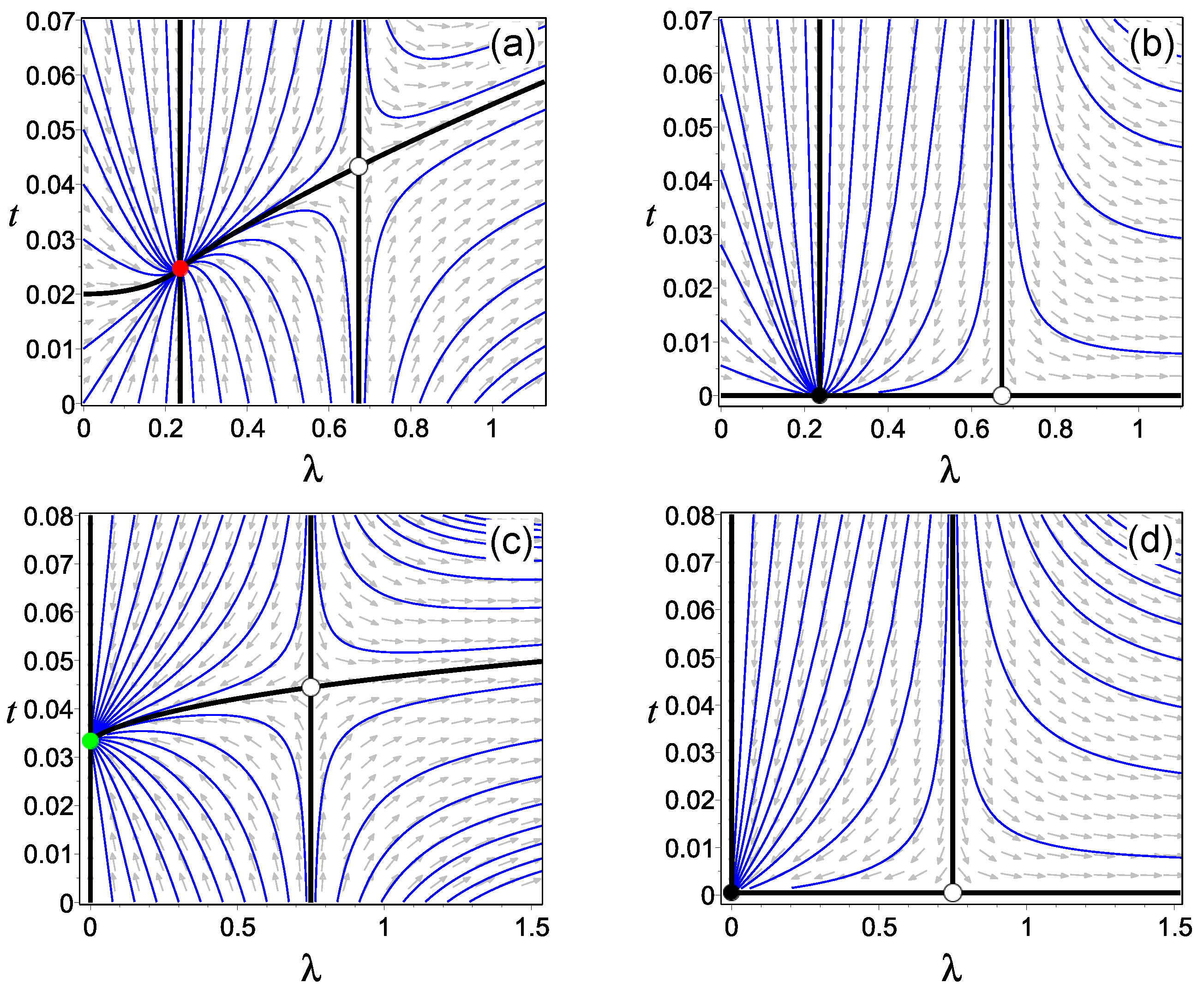
The trajectories of the renormalization group (RG) are given by the equations:

$$\begin{array}{ccc}\hfill {\displaystyle \frac{\mathrm{d}t}{\mathrm{d}z}}=\epsilon t-[N-2-\lambda (k-1)]t^2,& & t\left(0\right)=t_0,\hfill \end{array}$$

(50)

$$\begin{array}{ccc}\hfill {\displaystyle \frac{\mathrm{d}\lambda }{\mathrm{d}z}}=t\left[{\lambda }^2(N-1)-\lambda (N-2)+{\displaystyle \frac{k-2}{4}}\right],& & \lambda \left(0\right)={\lambda }_0.\hfill \end{array}$$

(51)

Then, the separatrices in Figure 1, passing through the points $(0;\epsilon ⁄(N-2\left)\right)$, $({\lambda }_{-};t_{-})$ and $({\lambda }_{+};t_{+})$, are obtained numerically by integrating (50) and (51). It can be seen that in the case of $2<k<N$ and $d>2$, the point $({\lambda }_{-};t_{-})$, at which the four phases meet, seems tetracritical (red circle in Figure 1a). Note that at $k=2$, such tetracriticality disappears, and the point $({\lambda }_{-};t_{-})=(0;\epsilon ⁄(N-2))$ becomes bicritical (green circle in Figure 1c). Finally, at $d=2$ and fixed $\lambda$, phase transitions by varying temperature t are not observed (see Figure 1b,d), although the sink–saddle pair still exists.

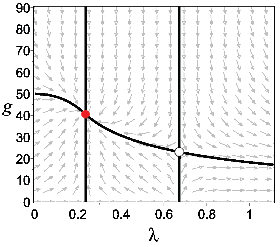
By introducing the quantity $g=1/t$, associated with the conductivity in some models, and the corresponding beta function ${\beta }_g\equiv \mathrm{d}g/\mathrm{d}z=-g^2{\beta }_t(t=1/g)$, we complement the case in Figure 1a with the behavior of g in Figure 2.

Critical exponents. As indicated above, the critical point—a stable fixed point (sink)—is given by the parameters $({\lambda }_{-};t_{-})$. By fixing $\lambda ={\lambda }_{-}$, and thereby reducing the Stiefel manifold to an Einstein manifold (with proportionality between the Ricci tensor and the metric), it is easy to calculate the critical exponent $\nu$ (and $\eta$) in the one-loop approximation for $2\le k<N$ and $\epsilon >0$. Under these conditions, there exists a positive critical temperature $t_c=t_{-}$, the determination of which provides [15]:

$${\displaystyle \frac{1}{\nu }}=-{\beta }_t^{\prime }\left(t_c\right)=\epsilon +O\left({\epsilon }^2\right).$$

(52)

This agrees with the known result for the Grassmannian $SO\left(N\right)⁄\left[SO\right(N-k)\times SO(k\left)\right]$ with the Einstein property.

Focusing primarily on the specifics of renormalizing the metric rather than the field, based on the results in Appendix B.2 we may estimate the exponent $\eta$ similarly to [4]:

$$\begin{array}{ccc}\hfill \eta & =& \zeta \left(t_c\right)-\epsilon \hfill \\ & =& \epsilon \left[{\displaystyle \frac{N-k+(k-1)/\left(2{\lambda }_{-}\right)}{N-2-{\lambda }_{-}(k-1)}}-1\right]+O\left({\epsilon }^2\right).\hfill \end{array}$$

(53)

We observe that $\eta \to 0+O\left({\epsilon }^2\right)$ for large N, and furthermore, when $k=1$, this expression yields the previously established value [4].

Other critical exponents can be found using the scaling and hyperscaling relations:

$$\alpha =2-\nu d,\beta =\nu {\displaystyle \frac{d-2+\eta }{2}},\gamma =(2-\eta )\nu ,\delta ={\displaystyle \frac{d+2-\eta }{d-2+\eta }}.$$

(54)

Their values for the model in the one-loop approximation are given in the

Table 1. Critical exponents for the temperature transition at $\lambda ={\lambda }_{-}(N,k)$.

Parameters	$N>2$, $k=1$	$N>2$, $k=2$	$N=12$, $k=9$
d	$2+\epsilon$	$2+\epsilon$	$2.2$
$t_c$	$\epsilon /(N-2)$	$\epsilon /(N-2)$	$0.0247$
$\alpha$	$1-2/\epsilon$	$1-2/\epsilon$	$-9$
$\beta$	$(N-1)/\left[2\right(N-2\left)\right]$	$+\infty$	$1.2278$
$\gamma$	$2/\epsilon -1/(N-2)$	$-\infty$	$8.5443$
$\delta$	${\displaystyle \frac{(4+\epsilon )N-8-3\epsilon }{\epsilon (N-1)}}$	$-1$	$7.9589$
$\nu$	$1/\epsilon$	$1/\epsilon$	5
$\eta$	$\epsilon /(N-2)$	$+\infty$	$0.2911$

. It is worth noting that just the rightmost column shows clearly the dependence on k: that is easily seen if we put $N=12$ in the left neighboring (or $k=2$) column and then compare the values in both columns. It is also interesting to note that at $k=1$, the critical exponent $\beta$ does not depend on $\epsilon$, unlike all other exponents in this column. On the other hand, the critical exponents $\alpha$ and $\nu$ do not depend on N and are the same for any $k>0$.

5. Conclusions

In this work, starting from the field Lagrangian for the $(2+\epsilon )$-dimensional nonlinear sigma model on the real Stiefel manifold, we applied the background-field method and normal coordinates for the quantum treatment and obtained a renormalization group description of the renormalized model in terms of two effective or running (depending on the scaling parameter) charges. This result fully confirms the corresponding formulas for beta functions and the properties of the renormalization group behavior of the studied model, previously obtained [11,18] by applying a pure geometric approach to the general case of the matrix beta function of a nonlinear model on an arbitrary Riemannian manifold. The special tetracritical behavior—the presence of a tetracritical point common to four phases—requires further detailed study (of the symmetry properties, etc.) of each of these phases and the corresponding critical exponents. No less interesting is the subsequent application of the considered model to the description of the properties of real tetracritical physical systems, in particular to the problem of the possible coexistence and mutual influence of the phenomenon of (de)localization in a quasi-two-dimensional electronic system and the phenomenon of superconductivity, as well as other systems with two independent order parameters (see, e.g., Refs. [29,30] for two such examples of symmetry-based systems that manifest tetracritical behavior). More generally speaking, the obtained results may also be useful from the viewpoint of studying new classes of universality and their systematics in the physics of (multi)critical phenomena.