Abstract
This study is to correct magnetic saturation and wavelength shift in Full-disk Magnetograph (FMG) solar magnetic field measurements on the Advanced Space-based Solar Observatory (ASO-S) satellite. Due to its single-wavelength polarization data limitations, currently, FMG relies on linear calibration. We propose a residual network model to output a line-of-sight (LOS) magnetic field which is trained with HMI LOS magnetic fields as target, and FMG Stokes I, V data and LOS velocity components as inputs. Compared to traditional methods, our model achieves lower MAE, RMSE, and improved consistency with the target, while also demonstrating robustness to wavelength shift, offering more accurate magnetic field measurements.
1. Introduction
The Advanced Space-based Solar Observatory (ASO-S) was launched on October 2022, with the scientific objective of studying the relationships between the solar magnetic field, solar flares, and coronal mass ejections [1]. The Full-disk Magnetograph (FMG) is one of the three payloads on the ASOS, with the work spectrum line as Fe I 5324.19 Å line [2]. As a filter-type spectrometer, the FMG performs polarization observations on one side of the line center in its regular mode, at the position of about −0.08 Å. The regular observation of FMG has a temporal resolution of approximately 2 min, a spatial resolution of about 1.5 arcseconds, and a pixel size of approximately 0.5 arcseconds [2]
The single-wavelength point polarization data of FMG do not allow magnetic field inversion and can only obtain magnetic field data through linear calibration. Under the weak-field approximation, the line-of-sight (LOS) magnetic field can be derived from the circular polarization parameter:
where is the calibration coefficient, V and I are the components of Stokes, and is the LOS magnetic field. The linear calibration coefficient used for FMG on-orbit data is [3]. However, linear calibration encounters the issue of magnetic saturation, leading to incorrect calibration results for strong magnetic fields. Xu et al. [4] compared the LOS magnetic fields of FMG and the Helioseismic and Magnetic Imager (HMI), highlighting the magnetic saturation effect [5,6].
Additionally, as a spaceborne instrument, FMG faces challenges in magnetic field calibration due to wavelength shifts caused by the Doppler effect. The relative motion between the detector and the Sun results in a shift in the observed wavelength position. The calibration coefficients vary at different wavelength positions, meaning that the calibration relationship changes over time as the LOS component of the satellite’s orbital velocity changes. This effect is further complicated by the influence of the LOS component of the Sun’s rotational velocity. As a result, different calibration relationships may exist across various positions on the solar disk at the same observation time.
In traditional calibration methods, the issue of wavelength shift is typically addressed using a tabulation approach. Calibration coefficients are tabulated for different relative velocities, and the calibration relationship for various regions on the solar disk is determined by referencing these tables based on the LOS component of the orbital velocity at the time of observation. This method requires a sufficient amount of observational data, covering the entire range of orbital velocities, to accurately calculate the calibration coefficients.
To address the issues of magnetic saturation and wavelength shift in single-wavelength calibration, we use the Convolutional Neural Network (CNN) method in machine learning (ML) to construct a calibration model. The model is trained to learn the mapping relationship between single-wavelength polarization data and LOS magnetic field obtained from multi wavelength polarization inversion. We hope that the trained model will output the right LOS magnetic field without the influence of magnetic saturation and wavelength drift based on single-wavelength observations.
Given the powerful nonlinear fitting capabilities of machine learning, many researchers have attempted to apply those machine learning methods to magnetic field inversion and calibration since the beginning of the 20th century. Carroll and Saude [7] were among the first to utilize a multi-layer perceptron (MLP) for fitting the Stokes inversion of 81 wavelength points, allowing them to derive various parameters, including the total magnetic field [8,9]. Socas-Navarro [10] introduced an inversion method based on principal component analysis (PCA), which they also employed for preprocessing the neural network input data [11,12]. This approach effectively reduced data dimensionality, enhancing the speed of network predictions (see [10]). Carroll et al. [13] applied MLP to model the radiative transfer involved in Zeeman–Doppler imaging and Stokes profile inversion. In another study, Teng [14] leveraged statistical machine learning techniques based on the Mercer kernel to deduce the photospheric magnetic field from polarization data. For the first time, Asensio Ramos and Díaz Baso [15] utilized CNN in the calibration of solar magnetic fields. Guo et al. [16,17] employed both MLP and CNN for magnetic field inversion using Hinode/SP data, showcasing the practicality of neural networks in single-wavelength magnetic field calibration [18]. Higgins et al. [19] applied a UNet architecture for inverting HMI data and implemented regression-by-classification in their output process. Mistryukova et al. [20] designed an end-to-end inversion code based on neural networks and the Milne–Eddington (ME) model, providing both the stellar atmosphere parameter estimation and their uncertainty intervals. Before the launch of FMG, we simulate the on-orbit single-wavelength point polarization observations using HMI data and develop a calibration method based on neural networks [21].
In Section 2, we introduce the data sources used to construct the dataset and the data preprocessing methods. In Section 3, we introduce the CNN model we used and the training related methods, and present the output of the model. In Section 4, we examine in detail the correction effect of magnetic saturation and wavelength shift in the output of the CNN model.
2. Data and Preprocess
2.1. Data
We use level 1 FMG data as input for the model, which includes Stokes parameters for the four channels of . Compared to level 0 data, these level 1 data are corrected for dark field effects and cross-talk effects. Due to the correlation between LOS magnetic field parameters and Stokes , we select I and V channels as inputs for the model.
In order for the model to calculate the magnetic field parameters corresponding to the polarization parameters, we need to provide the corresponding magnetic field parameters as targets during the training process. And we hope that there is no magnetic saturation effect or spectral line drift in these target LOS magnetic fields. We consider using data from HMI as the output target. HMI performs 6-point polarization observations at the 6173.34 Å spectral line, outputting LOS magnetic fields with a 45 s cadence and 6-point polarization and vector magnetic field data with a 720 s cadence [5,22]. The HMI vector magnetic field is derived by solving the Milne–Eddington (ME) model using the VFISV code [23], which avoids the issues of magnetic saturation and wavelength shift that occur with single-point observations.
We need to use a monochromatic image to register the HMI and FMG images. For this purpose, we select 720 s data from HMI to generate targets in the dataset. The 720 s data of HMI include polarization parameters for six complete wavelength points, as well as multiple magnetic field and atmospheric parameters. These parameters include the total magnetic field, inclination angle, and azimuth angle. We calculate the LOS magnetic field from these. The processing of HMI data and cross instrument alignment methods are detailed in the preprocessing section.
Using HMI as the target for neural network learning does not mean converting the FMG polarization image into the HMI longitudinal magnetic map; the two instruments operate on different spectral lines, and this calibration method is expected to retain different information in the 5324 Å polarization map from that in the 6173 Å magnetic map; in addition, a 2 min cadence (FMG observation cadence) longitudinal magnetic map with the same calibration relationship as the HMI 720 S data can be obtained.
Due to the large volume of data, we select one day every five days from May to August to create the dataset. Data from 24 days are selected and split into training, validation, and test sets in a 6:2:2 ratio, resulting in 1246, 462, and 423 groups of FMG-HMI images, respectively. Table 1 lists the data sources used to construct our dataset. After preprocessing and cropping, the final numbers of 256 × 256 pixel sized image data groups in the three datasets are 4099, 1424, and 1419, respectively.

Table 1.
Data sources.
2.2. Preprocess and Dataset
The preprocessing required for FMG1.5 level data before entering the network only includes normalization, image cropping, and co-alignment. The I channel divides each image by its own median to scale to the order of 1. The V channel is actually V/I data, mostly on the order of to . We scale the V channel to the order of 1 by multiplying it with a constant coefficient.
Additionally, to account for the Doppler effect, we need to input the velocity information into the network. The relative velocity in this observation is caused by the LOS component of the Sun’s surface rotational velocity and the satellite’s orbital velocity.
The LOS component of the satellite’s orbital velocity is obtained from the FITS header of the data, where the keyword ‘OBSVR’ represents this value. For a given moment’s data, we expand this value into an image with the same dimensions as the observational data, where each pixel holds the same value.
The Sun’s differential rotational velocity is calculated using the theoretical formula. By applying the map function from Sunpy to the data, the longitude and latitude of each pixel on the solar disc can be determined [24]. The latitude and longitude images are projection-corrected and adjusted for the B-angle. B-angle refers to the angle between the solar axis and the camera plane caused by the angle between the solar equatorial plane and the ecliptic plane. It is also equivalent to the latitude of the heliocentric position on the image. These latitude and longitude images are then used in the rotation formula to produce a rotational velocity image, with the velocity direction aligned along the solar disc’s latitudinal lines. The parameters of solar differential rotation come from Newton and Nunn [25], Timothy et al. [26]. This velocity is projected onto the line of sight of the detector to obtain the LOS component of the rotational velocity, which we refer to as the ‘ROTVR’ image, consistent with the ‘OBSVR’ image.
We use ROTVR and OBSVR as two additional channels for the model input. Similarly, these two channels are normalized during input by dividing them by a scaling factor, which we set to 3000 m/s.
Most of the pixels on the solar surface are quiet regions with weak magnetic fields, so directly inputting the solar surface image during training would waste a lot of training time. To generate the dataset, we crop the images into smaller sizes around the active area. Due to the need for a target image that corresponds to the local input image, we perform a cropping operation in the step of aligning FMG with HMI.
One of the challenging steps in constructing the dataset is aligning the FMG and HMI images. To achieve a sufficiently precise alignment, we design an iterative alignment method that undergoes multiple iterations. This method is similar to the one used in processing SUTRI data [27].
We first use the SIFT algorithm to align the full-disk HMI images with the FMG images [28]. For the majority of the data, this approach results in alignment errors within dozens of pixels. However, due to the nature of the data, some images cannot be matched effectively by SIFT, either because they lack enough feature points or because incorrect feature point matches are made. This often leads to an exaggerated transformation matrix. We apply a set of thresholds of transformation matrices to discard these datasets that cannot be initially aligned.
To obtain precisely aligned FMG-HMI data pairs, we perform a second, more accurate alignment on the cropped images. We use cross-correlation to achieve precise alignment of active region images. The alignment process provides the relative displacement between images and the cross-correlation coefficient after alignment.
Some images are difficult to align due to factors such as differing PSF functions and distortions from different instruments. We apply a cross-correlation coefficient threshold to discard those active region images that cannot be precisely aligned.
3. Method and Result
3.1. CNN Method
The model we use is residual network (ResNet), a type of CNN [29]. ResNet introduces shortcut connections to form residual blocks on top of the CNN architecture. This design helps avoid the vanishing gradient problem during backpropagation and is widely used in image processing networks.
The residual blocks we use include two 3 × 3 convolutional layers and two activation layers. There are a total of 16 residual blocks in the network, including two convolutional layers for the input and output layers. The last convolutional layer serves directly as the network output and is a 1 × 1 convolutional layer, outputting the LOS field. The network architecture is the same as that used in Hu, Ziyao et al. [21], who showed that by using LeakyReLU as the activation function, one may prevent the appearance of the so-called dead neurons. Using LeakyReLU as the activation function helps prevent the issue of neuron death.
The input to the network consists of four-channel images: Stokes I, V, and two velocity images, OBSVR and ROTVR. In the cropped data, each pixel of the ROTVR channel is the LOS component of the rotation velocity obtained by theoretical calculation; while each pixel in the single data of the OBSVR channel is equal, which is the LOS component of the orbital velocity. The output is a single-channel LOS magnetic field image. All input images are normalized and unitless, while the output image is in gauss units.
The network is trained using 256 × 256 32-bit floating-point images. The purpose of using cropped images for training is twofold: first, to balance the dataset by increasing the proportion of strong magnetic field pixels in the dataset; and second, to enable the use of a larger batch size, which helps the network converge more quickly.
Although cropping images around active regions removes most of the quiet Sun pixels, there remains an order-of-magnitude difference between the number of quiet and active region pixels in the cropped data. This is especially true for very strong magnetic field pixels, such as those above 3000 G, which are underrepresented. This imbalance means that the loss function calculation is primarily influenced by weak magnetic fields. As a result, the optimized network might exhibit large errors in regions with strong magnetic fields, while still achieving a sufficiently low overall loss function for the entire image.
To address this, we use a weighted loss function that accounts for the distribution of different magnetic field strengths in the dataset. As proposed by Hu, Ziyao et al. [21], we apply the negative logarithm of the probability of the field strength B as the pixel weight. The loss function based on mean absolute error (MAE, L1 loss) is as follows:
where is the value of pixel i in target, is the value of pixel i predicted by the network, and is the weight of the pixel, which is related to the field strength at this point. We use the -log as , where is the probability of the field strength B in the training set. Compared to mean squared error loss (MSE, L2 loss), although MAE converges more slowly, it is less affected by outliers and is more robust. MAE and MSE are two commonly used loss functions when training neural networks, which are and , respectively.
3.2. Result
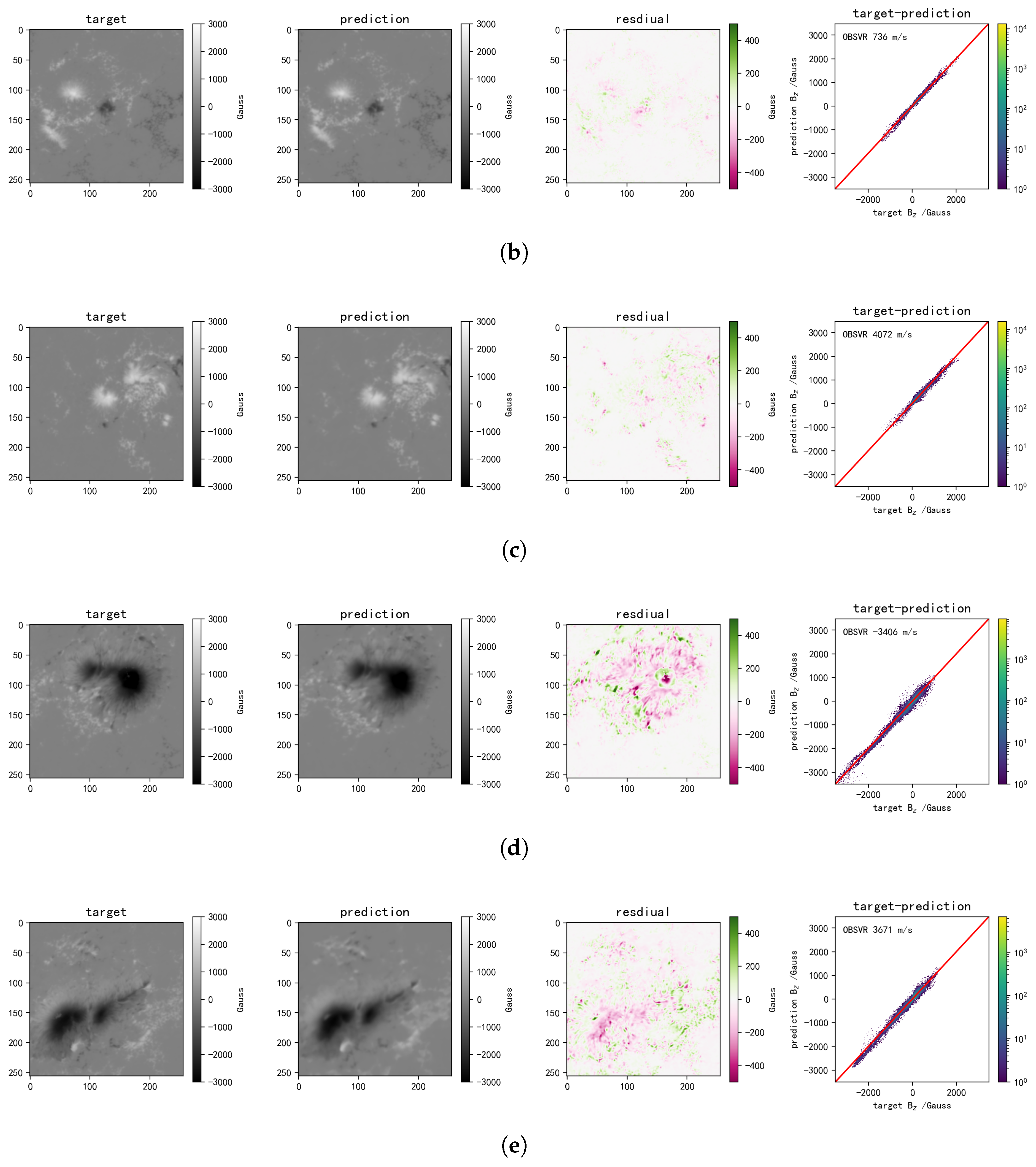
In order to assess the accuracy of the CNN model in calibrating FMG data, we conduct a series of tests and evaluations on the model. The model is used to predict the LOS magnetic field images for data in the test set, and the results are compared with the target. The data in the test set are not included in the network training, nor are they used for adjusting hyperparameters. Figure 1 displays some of the prediction results from the test set. These results include observations at different orbital velocities. The scatter density plot illustrates the predictions versus target for each pixel in the test data. The red 45-degree line in the plot indicates perfect agreement between the predictions and target.

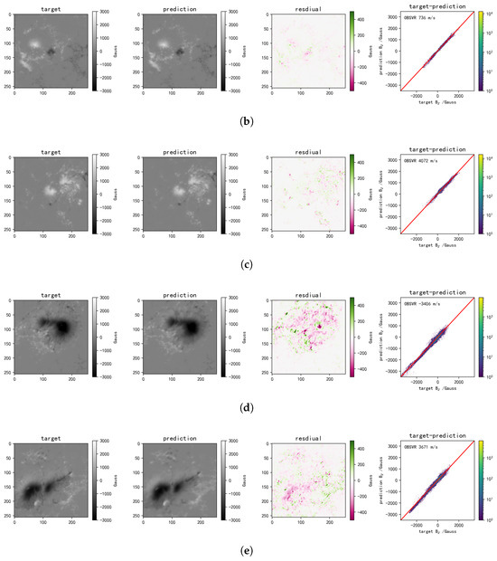
Figure 1.
Examples from the test set. The (a–e) panels represent sunspots in the test set at different dates and orbital velocities. Each panel displays the label image, the model prediction image, the residual image, and the scatter plot. The OBSVR value for each panel is indicated in the scatter plot. The OBSVR of panels a to e are −445 , 736 , 4072 m/s, −3406 , and 3671 respectively.
In the test set, the MAE between the CNN-predicted LOS magnetic field and the target is 19.87 G, the Root Mean Square Error (RMSE) is 38.61 G, the coefficient of determination is 0.969, and the correlation coefficient r is 0.985. RMSE is the square root of MSE and has the same units as the observed value. The definition of the coefficient of determination is Equation (3):
here and have the same meaning as Formula (2), and the is the average value of target . The parameter is usually used to measure the correlation between the result of the regression and the target. In regression tasks, the coefficient of determination can be used to measure the proportion of the variance in the dependent variable that is predictable from the independent variables, essentially indicating how much of the target’s variation is explained by the model’s predictions; On the other hand, the correlation coefficient describes the degree of the linear relationship between the predictions and the targets.
4. Discussion
In order to evaluate the performance of CNN methods in single-wavelength calibration tasks, we conduct the following series of analyses in this section. These analyses include examining the LOS magnetic field from linear calibration, calibration using CNN, and the original HMI data, and the correlations between them; examining the relationship between CNN output and target at different speeds to evaluate the stability of CNN under different wavelength shifts; and tracking the I images, the linear calibration, and CNN output of an active region at different speeds in orbit, influenced by OBSVR. In addition, we discuss the mid-value of the quiet region and magnetic flux of the active region with different OBSVR.
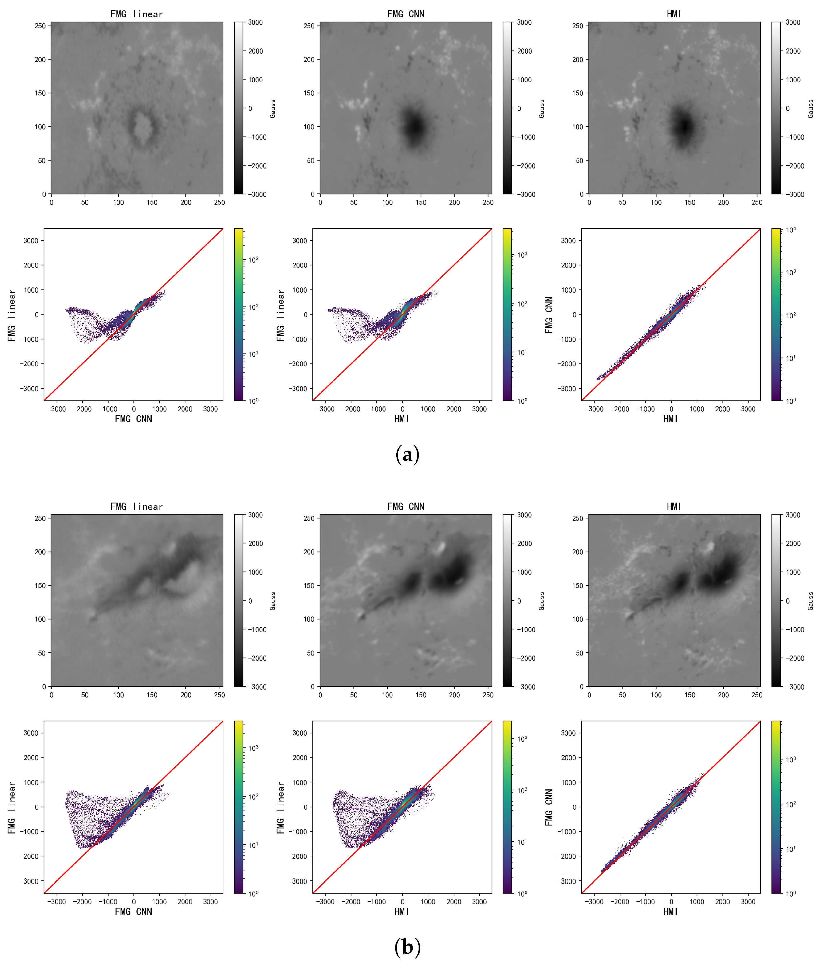
Figure 2 demonstrates the correction of the magnetic saturation effect using the CNN calibration method. We find two examples from the test set where FMG experienced magnetic saturation during observation and compare the LOS magnetic fields obtained using linear calibration and the CNN method with the HMI LOS magnetic field. Additionally, scatter plots are created for each pair of these three magnetic fields to assess their correlation. It can be seen that in regions with stronger magnetic fields, such as the sunspot centers, the linear calibration shows clear signs of magnetic saturation. In contrast, the LOS magnetic field obtained using the CNN method no longer exhibits saturation and shows a higher correlation with the HMI magnetic field derived from inversion.
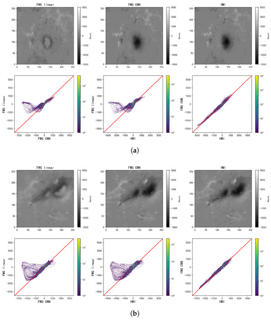
Figure 2.
Two examples of magnetic saturation correction in active regions are presented. Each panel shows the LOS magnetic field obtained by FMG using both linear calibration and the CNN model, along with the LOS magnetic field from HMI. Scatter plots comparing the LOS magnetic fields from each pair are also provided. Panel (a) corresponds to NOAA AR13394, from 9 August 2023, at 00:12:48, while panel (b) corresponds to NOAA AR13363, from 15 July 2023, at 02:00:05.
To assess the calibration accuracy of our model under different spectral line shifts, we plot scatter plots of the model’s output at various relative motion velocities. As shown in Figure 3, each panel represents a scatter plot of the model’s output versus the target at different velocities, with color indicating the density of the points. Similarly, the closer the points are to the red line, the better the prediction matches the target. The velocity labeled in each panel is the sum of OBSVR and ROTVR for a pixel in the data. It can be observed that the distribution of predictions remains relatively consistent across different velocities. This indicates that the prediction by the CNN model is almost unaffected by the wavelength shift.

Figure 3.
Scatter plots of the network predictions versus the target at different Doppler velocities. The twelve panels statistically cover the OBSVR values from −6000 to 6000 , binned in 1000 intervals.
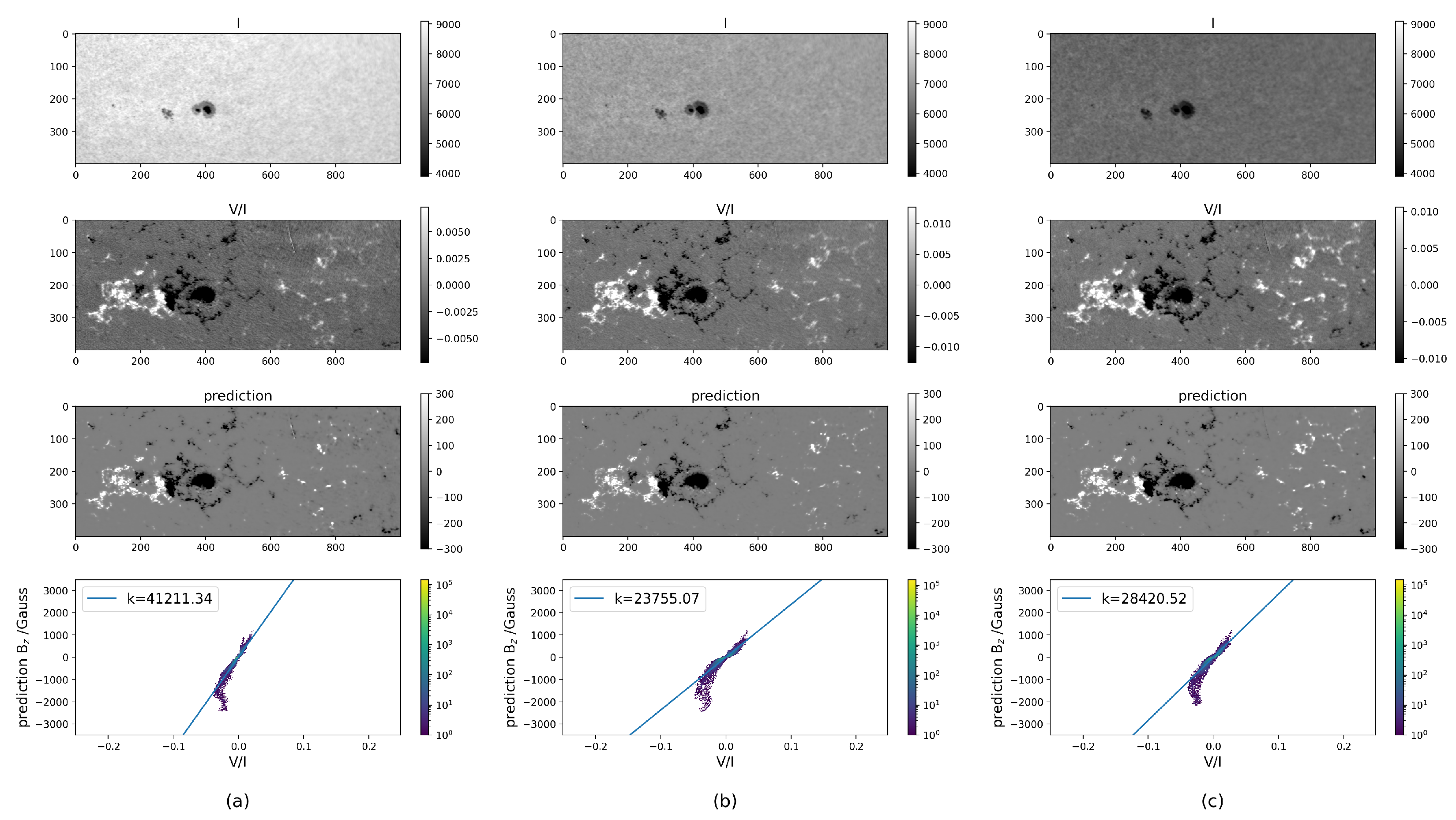
In Figure 4, we present the output results of the network model during a single orbit. The data are from 13 June 2023, and we track and plot the active region NOAA AR13331. The three timestamps shown in the figure correspond to the FMG OBSVR values of 4109 , −6 , and −3707 . These represent the maximum positive and negative orbital velocities, as well as a moment when the velocity is near zero. Due to a period of time when the satellite is in Earth’s shadow, the chronological order of the images is a, c, and b.
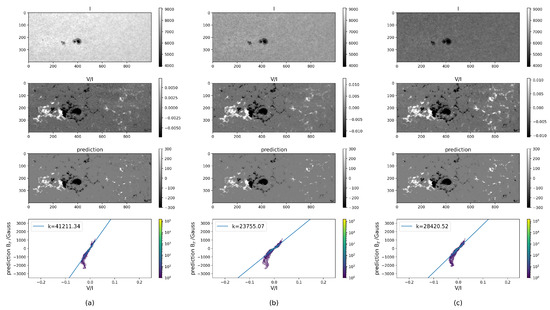
Figure 4.
The magnetic field of NOAA AR13331 at different orbital velocities, with data from 13 June 2023. Each row shows Stokes I, Stokes V/I, the magnetic field predicted by the CNN model, and a scatter plot of V/I against the CNN-predicted magnetic field for that time. The OBSVR values for columns (a), (b), and (c) are 4109 , −6 , and −3707 , respectively.
It can be observed that the monochromatic images captured by FMG show significant brightness changes at these three timestamps. In the V/I images, some small magnetic field structures exhibit different areas and intensities at different velocities. However, the CNN output at each timestamp displays a more stable background, magnetic field strength, and structure. The variations in I and V/I images at different times are due to the impact of spectral line shifts. When the actual observed wavelength is closer to the line center, the I image appears darker, and when it is farther, the image appears brighter. In V and V/I images, the relationship between the wavelength position and pixel Digital Number (DN) value is more complex. The figure demonstrates that the CNN model, compared to linear calibration, is better suited for handling the calibration relationship under different orbital velocities.
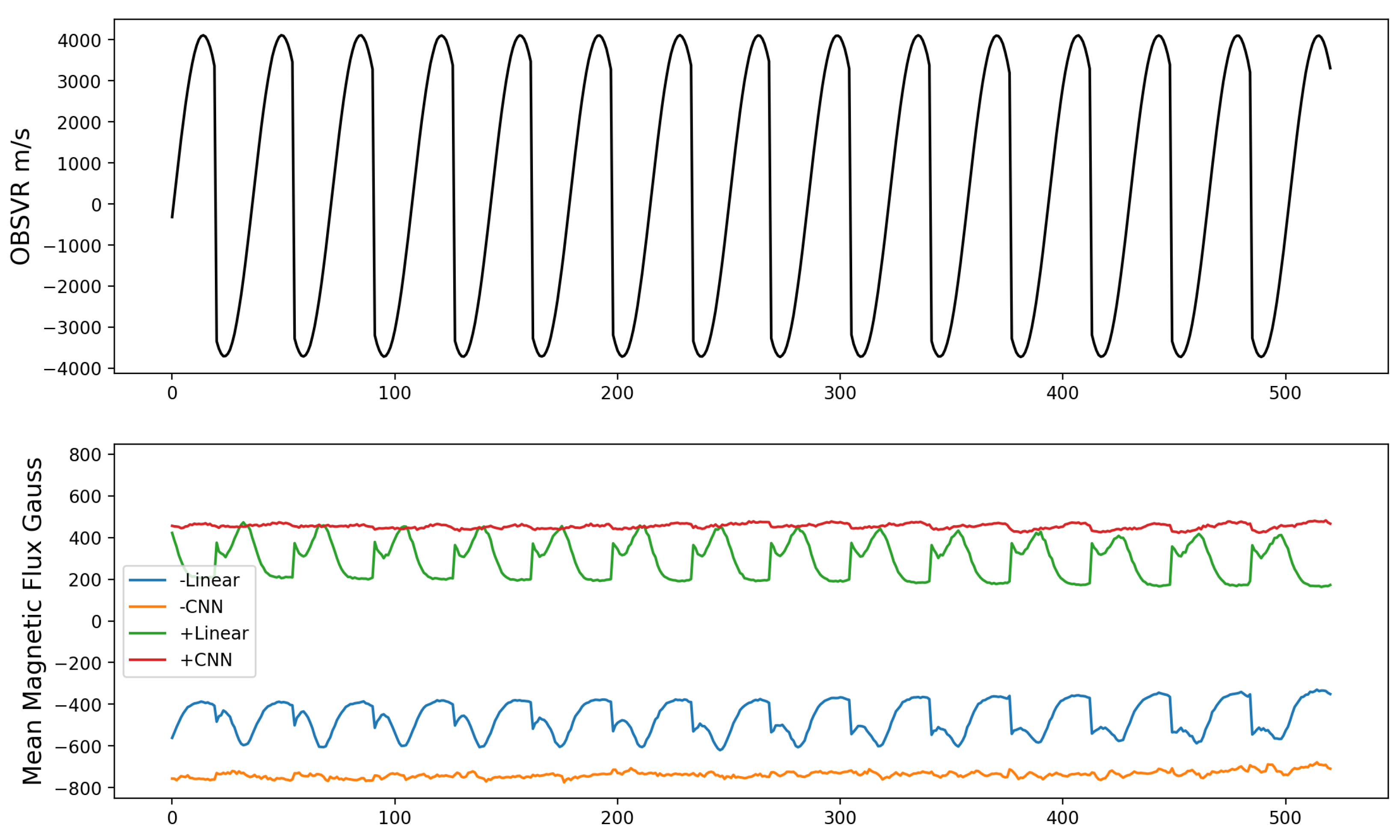
We track the changes in magnetic flux of the AR13331 in the data of two calibration methods on 13 June 2023 with different OBSVR. We separately calculate the mean magnetic flux of LOS magnetic greater than 300 G and the mean magnetic flux of magnetic fields less than negative 300 G. The mask for selecting pixels is pixels in the CNN output with an absolute value greater than 300 G. The positive and negative mean magnetic fluxes of two LOS magnetic fields and their corresponding orbital velocities are shown in Figure 5. The selection of pixels depending on the absolute values of CNN output allows the mean magnetic flux to be less than the threshold of 300 G. In addition, due to the lack of observation for a portion of the time in the orbit, there are jumps in the curve. We can see that the absolute value of the CNN flux is greater than that of the linearly scaled flux. This is because of the magnetic saturation effect, which results in a smaller linear calibration magnetic field at the center of the sunspot. The linear calibration magnetic flux exhibits periodic oscillations with the OBSVR, and the fluctuation amplitude is much larger than that of the CNN magnetic flux.
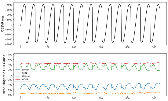
Figure 5.
The mean magnetic flux of NOAA AR13331 at different orbital velocities, with data from 13 June 2023. Each panel shows OBSVR; positive and negative mean magnetic flux of linear calibration and CNN. Positive and negative pixels in the linearly calibrated LOS magnetic field are denoted by blue and green curves showing their mean flux densities, while yellow and red curves represent equivalent measurements from the CNN-processed LOS field.
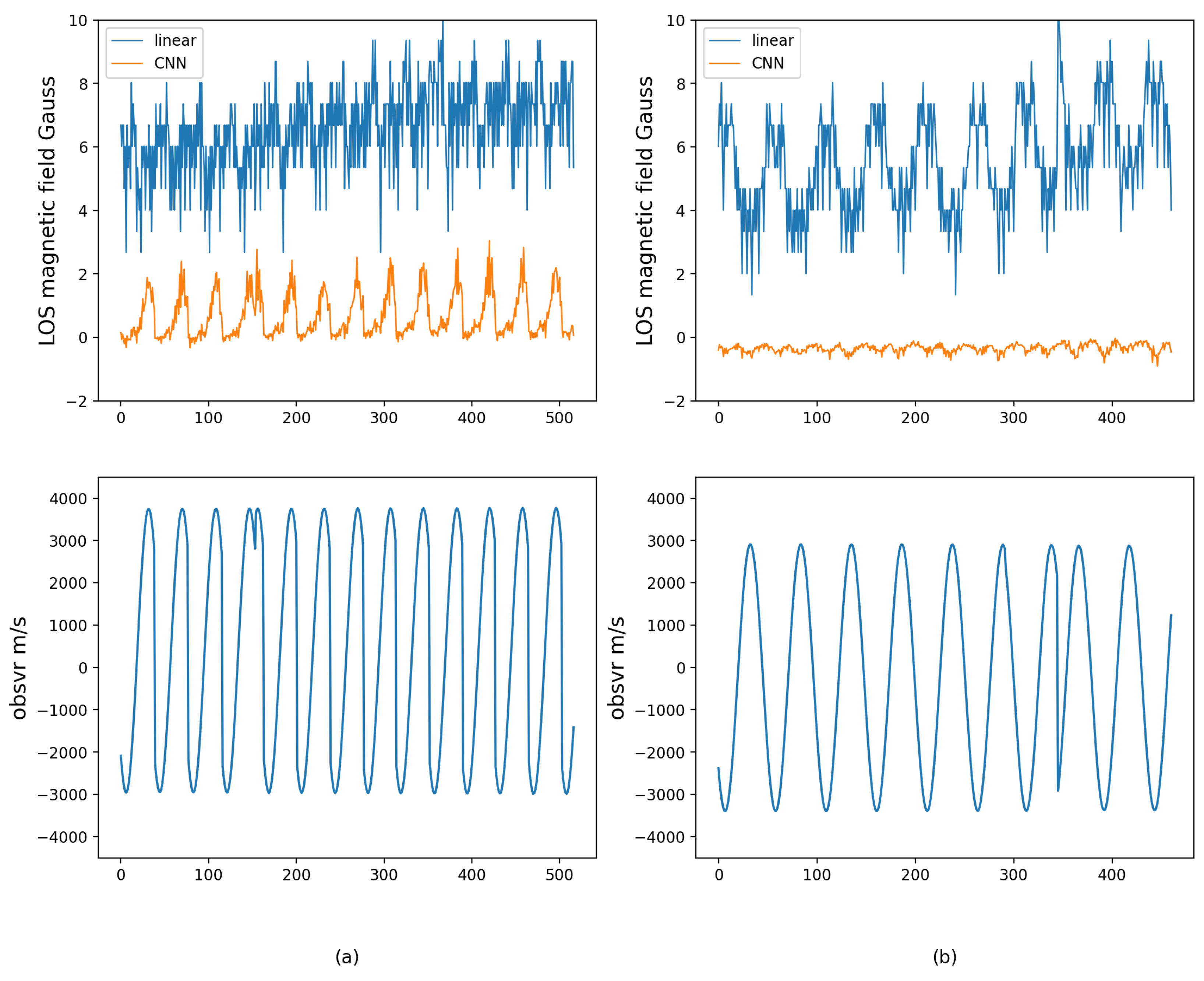
In Figure 6, we present the variation of median values in the quiet regions at different times of the day. We statistically analyze the data from 13 May and 7 August 2023 which are displayed as panels a and b, respectively. In the first graph of each panel, we show the median of the LOS magnetic field for pixels below 300 G at different times of the day, and in the second graph, we present the corresponding OBSVR of the data. It can be observed from the graphs that both the linear calibration and the CNN-derived median values in the quiet regions exhibit periodic changes with OBSVR. From the statistical results, we believe that there is a bias in the magnetic field observed by the instrument. The linear calibration method reveals the magnitude of this bias and its variation with OBSVR. However, the bias in the LOS field obtained by the CNN model is smaller and more stable with respect to the OBSVR.
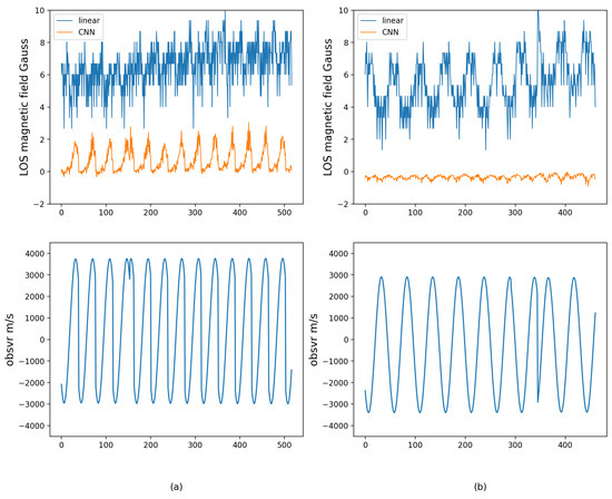
Figure 6.
LOS bias derived from the median LOS magnetic field in quiet region at different times of the day, showing its variation with the OBSVR. Panel (a) is from 13 May 2023; panel (b) is from 7 August 2023. The blue and yellow traces in the upper panel correspond to the linear-calibrated and CNN-processed LOS magnetic fields, respectively.
In addition, the bias of the quiet region of CNN on May 3rd shows much larger fluctuations than on 7 August. We believe this is due to a significantly large OBSVR. The OBSVR range on 3 May is −2986.82 m/s to 3769.77 m/s, while the range on 7 August is −3399.43 m/s to 2907.13 m/s. Positive velocity indicates that the instrument and the Sun are moving away from each other. Due to the conventional observation wavelength position being −0.08 Å, excessive positive velocity may cause the actual observation position to move beyond the spectral line width. In this case, the V/I signal becomes small enough to lower the signal-to-noise ratio. This causes the quiet region bias calculated by CNN to exhibit significant fluctuations at sufficiently high speeds.
5. Conclusions
To deal with the magnetic saturation and wavelength shift in the calibration of FMG LOS magnetic fields, we designed and provided a CNN-based single-wavelength nonlinear calibration method. Our model takes as input the Stokes I and V images from FMG level 1 data, along with the LOS components of the satellite orbital velocity and the solar rotational velocity. The labels used for training the model is the LOS magnetic field images from HMI 720 s data.
In the test set, the model’s prediction of the LOS magnetic field compared to the HMI LOS magnetic field used as labels has an MAE of 19.87 G, an RMSE of 38.61 G, and a coefficient of determination of 0.969. Our model effectively corrects the magnetic saturation effect in the FMG LOS magnetic field obtained from linear calibration, demonstrating good agreement with the HMI LOS magnetic field derived from VFISV. For data across different satellite speeds during an orbit, the model remains unaffected by brightness variations in the original data. By analyzing the variation of the mean magnetic flux in the active area with orbital velocity, we believe that the LOS magnetic field obtained by the CNN method is more stable than the linear calibration method when the OBSVR changes. We also tracked the median value of the quiet region, which serves as the bias of the magnetic field image, to observe how it changes with orbital speed throughout the day. The results indicate that our model exhibits smaller bias and lower fluctuations compared to linear calibration.
Through these analyses, we believe that in the single-wavelength LOS magnetic field calibration task, CNN solves the problem of magnetic saturation better than linear calibration and can adapt to different wavelength drifts. It is interesting that cross-instrument learning can correct biases in the data to a certain extent.
However, it should be noted that there are still some issues with the CNN method. Due to the limitations of single-wavelength data, some fluctuations may still be observed at extremely high speeds as can be seen from the bias in the quiet region. And this fluctuation can only be obtained at one of the maximum positive or negative velocities, depending on which side of the center line the observation position is on. In addition, the rotational speed of the solar surface is calculated based on theoretical formulas and is therefore influenced by the selection of differential rotation parameters. In subsequent work, we will use different differential rotation parameters to obtain the theoretical solar differential rotation velocity and compare the impact on the magnetic field calibration [30,31].
Author Contributions
Conceptualization, K.J. and J.G.; methodology, K.J. and Z.H.; software, Z.H.; validation, K.J., X.B., J.S., S.L. and Z.H.; formal analysis, Z.H.; investigation, Z.H.; data curation, Z.H.; writing—original draft preparation, Z.H.; writing—review and editing, all authors; visualization, Z.H.; supervision, Y.D. and X.B.; funding acquisition, K.J., Y.D., X.B. and J.S. All authors have read and agreed to the published version of the manuscript.
Funding
The National Key Research and Development Program of China under grant No. 2022YFF0503001, 2022YFF0503800, 2021YFA1600500 and the National Natural Science Foundation of China under grant No. 12273059, 12073077 and 12103034. Xianyong Bai is also supported by the Youth Innovation Promotion Association CAS (2023061).
Data Availability Statement
Conflicts of Interest
The authors declare no conflicts of interest.
References
- Gan, W.Q.; Zhu, C.; Deng, Y.Y.; Li, H.; Su, Y.; Zhang, H.Y.; Chen, B.; Zhang, Z.; Wu, J.; Deng, L.; et al. Advanced Space-based Solar Observatory (ASO-S): An overview. Res. Astron. Astrophys. 2019, 19, 156. [Google Scholar] [CrossRef]
- Deng, Y.Y.; Zhang, H.Y.; Yang, J.F.; Li, F.; Lin, J.B.; Hou, J.F.; Wu, Z.; Song, Q.; Duan, W.; Bai, X.Y.; et al. Design of the Full-disk MagnetoGraph (FMG) onboard the ASO-S. Res. Astron. Astrophys. 2019, 19, 157. [Google Scholar] [CrossRef]
- Bai, X.; Deng, Y.; Zhang, H.; Yang, J.; Li, F.; Su, J.; Liu, S.; Song, Y.; Ji, K.; Huang, Y.; et al. Calibration and Performance of the Full-Disk Vector MagnetoGraph (FMG) on Board the Advanced Space-Based Solar Observatory (ASO-S). Sol. Phys. 2024, 299, 157. [Google Scholar] [CrossRef]
- Xu, H.; Su, J.; Liu, S.; Deng, Y.; Yang, S.; Bai, X.; Chen, J.; Wang, X.; Yang, X.; Song, Y.; et al. Comparison of Line-of-Sight Magnetic Field Observed by ASO-S/FMG, SDO/HMI and HSOS/SMAT. Sol. Phys. 2024, 299, 17. [Google Scholar] [CrossRef]
- Schou, J.; Scherrer, P.H.; Bush, R.I.; Wachter, R.; Couvidat, S.; Rabello-Soares, M.C.; Bogart, R.S.; Hoeksema, J.T.; Liu, Y.; Duvall, T.L.; et al. Design and Ground Calibration of the Helioseismic and Magnetic Imager (HMI) Instrument on the Solar Dynamics Observatory (SDO). Sol. Phys. 2012, 275, 229–259. [Google Scholar] [CrossRef]
- Pesnell, W.D.; Thompson, B.J.; Chamberlin, P.C. The Solar Dynamics Observatory (SDO). Sol. Phys. 2012, 275, 3–15. [Google Scholar] [CrossRef]
- Carroll, T.A.; Staude, J. The inversion of Stokes profiles with artificial neural networks. Astron. Astrophys. 2001, 378, 316–326. [Google Scholar] [CrossRef][Green Version]
- Rumelhart, D.E.; Hinton, G.E.; Williams, R.J. Learning Representations by Back Propagating Errors. Nature 1986, 323, 533–536. [Google Scholar]
- Hornik, K.; Stinchcombe, M.; White, H. Multilayer feedforward networks are universal approximators. Neural Netw. 1989, 2, 359–366. [Google Scholar] [CrossRef]
- Socas-Navarro, H. Measuring solar magnetic fields with artificial neural networks. Neural Netw. 2003, 16, 355–363. [Google Scholar] [CrossRef]
- Pearson, K. LIII. On lines and planes of closest fit to systems of points in space. Philos. Mag. 1901, 2, 559–572. [Google Scholar]
- Hotelling, H. Analysis of a complex of statistical variables in principal components. J. Educ. Psychol. 1933, 24, 498–520. [Google Scholar]
- Carroll, T.A.; Kopf, M.; Strassmeier, K.G. A fast method for Stokes profile synthesis. Radiative transfer modeling for ZDI and Stokes profile inversion. Astron. Astrophys. 2008, 488, 781–793. [Google Scholar] [CrossRef]
- Teng, F. Application of Kernel Based Machine Learning to the Inversion Problem of Photospheric Magnetic Fields. Sol. Phys. 2015, 290, 2693–2708. [Google Scholar] [CrossRef]
- Asensio Ramos, A.; Díaz Baso, C.J. Stokes inversion based on convolutional neural networks. Astron. Astrophys. 2019, 626, A102. [Google Scholar] [CrossRef]
- Guo, J.; Bai, X.; Deng, Y.; Liu, H.; Lin, J.; Su, J.; Yang, X.; Ji, K. A Non-Linear Magnetic Field Calibration Method for Filter-Based Magnetographs by Multilayer Perceptron. Sol. Phys. 2020, 295, 5. [Google Scholar] [CrossRef]
- Guo, J.; Bai, X.; Liu, H.; Yang, X.; Deng, Y.; Lin, J.; Su, J.; Yang, X.; Ji, K. A nonlinear solar magnetic field calibration method for the filter-based magnetograph by the residual network. Astron. Astrophys. 2021, 646, A41. [Google Scholar] [CrossRef]
- Suematsu, Y. Review of Hinode results. Astron. Nachrichten 2010, 331, 605–608. [Google Scholar] [CrossRef]
- Higgins, R.E.L.; Fouhey, D.F.; Zhang, D.; Antiochos, S.K.; Barnes, G.; Hoeksema, J.T.; Leka, K.D.; Liu, Y.; Schuck, P.W.; Gombosi, T.I. Fast and Accurate Emulation of the SDO/HMI Stokes Inversion with Uncertainty Quantification. Astrophys. J. 2021, 911, 130. [Google Scholar] [CrossRef]
- Mistryukova, L.; Plotnikov, A.; Khizhik, A.; Knyazeva, I.; Hushchyn, M.; Derkach, D. Stokes Inversion Techniques with Neural Networks: Analysis of Uncertainty in Parameter Estimation. Sol. Phys. 2023, 298, 98. [Google Scholar] [CrossRef]
- Hu, Z.; Ji, K.; Chen, J.; Deng, Y.; Su, J.; Bai, X.; Liu, S.; Guo, J.; Liu, J.; Wintoft, P. Calibration scheme for space-borne full-disk vector magnetograph under the influence of orbiter velocity. A&A 2022, 666, A93. [Google Scholar] [CrossRef]
- Norton, A.A.; Graham, J.P.; Ulrich, R.K.; Schou, J.; Tomczyk, S.; Liu, Y.; Lites, B.W.; Ariste, A.L.; Bush, R.I.; Socas-Navarro, H.; et al. Spectral Line Selection for HMI: A Comparison of Fe I 6173 Å and Ni I 6768 Å. Sol. Phys. 2006, 239, 69–91. [Google Scholar] [CrossRef]
- Borrero, J.M.; Tomczyk, S.; Kubo, M.; Socas-Navarro, H.; Schou, J.; Couvidat, S.; Bogart, R. VFISV: Very Fast Inversion of the Stokes Vector for the Helioseismic and Magnetic Imager. Sol. Phys. 2011, 273, 267–293. [Google Scholar] [CrossRef]
- The SunPy Community; Barnes, W.T.; Bobra, M.G.; Christe, S.D.; Freij, N.; Hayes, L.A.; Ireland, J.; Mumford, S.; Perez-Suarez, D.; Ryan, D.F.; et al. The SunPy Project: Open Source Development and Status of the Version 1.0 Core Package. Astrophys. J. 2020, 890, 68. [Google Scholar] [CrossRef]
- Newton, H.W.; Nunn, M.L. The Sun’s rotation derived from sunspots 1934-1944 and additional results. Mon. Not. R. Astron. Soc. 1951, 111, 413. [Google Scholar] [CrossRef]
- Timothy, A.F.; Krieger, A.S.; Vaiana, G.S. The Structure and Evolution of Coronal Holes. Sol. Phys. 1975, 42, 135–156. [Google Scholar] [CrossRef]
- Bai, X.; Tian, H.; Deng, Y.; Wang, Z.; Yang, J.; Zhang, X.; Zhang, Y.; Qi, R.; Wang, N.; Gao, Y.; et al. The Solar Upper Transition Region Imager (SUTRI) Onboard the SATech-01 Satellite. Res. Astron. Astrophys. 2023, 23, 065014. [Google Scholar] [CrossRef]
- Lindeberg, T. Scale Invariant Feature Transform. Scholarpedia 2012, 7, 10491. [Google Scholar] [CrossRef]
- He, K.; Zhang, X.; Ren, S.; Sun, J. Deep Residual Learning for Image Recognition. In Proceedings of the 2016 IEEE Conference on Computer Vision and Pattern Recognition (CVPR), Las Vegas, NV, USA, 27–30 June 2016; pp. 770–778. [Google Scholar] [CrossRef]
- Kharayat, H.; Singh, J.; Priyal, M.; Ravindra, B. Equator to Pole Solar Chromospheric Differential Rotation Using Ca-K Features Derived from Kodaikanal Data. Astrophys. J. 2024, 968, 53. [Google Scholar] [CrossRef]
- Permata, K.; Herdiwijaya, D. The Measurement of Solar Differential Rotation from Proper Motion of Individual Sunspots. J. Phys. Conf. Ser. 2019, 1231, 012019. [Google Scholar] [CrossRef]
Disclaimer/Publisher’s Note: The statements, opinions and data contained in all publications are solely those of the individual author(s) and contributor(s) and not of MDPI and/or the editor(s). MDPI and/or the editor(s) disclaim responsibility for any injury to people or property resulting from any ideas, methods, instructions or products referred to in the content. |
© 2025 by the authors. Licensee MDPI, Basel, Switzerland. This article is an open access article distributed under the terms and conditions of the Creative Commons Attribution (CC BY) license (https://creativecommons.org/licenses/by/4.0/).


