Article

Improved Galaxy Morphology Classification with Convolutional Neural Networks

Department of Computer Science, Faculty of Mathematics and Computer Science, West University of Timisoara, 300223 Timisoara, Romania
*
Author to whom correspondence should be addressed.
Current address: Bulevardul Vasile Pârvan 4, 300223 Timisoara, Romania.
These authors contributed equally to this work.
Universe 2024, 10(6), 230; https://doi.org/10.3390/universe10060230
Submission received: 4 April 2024 / Revised: 13 May 2024 / Accepted: 16 May 2024 / Published: 21 May 2024
(This article belongs to the Section Galaxies and Clusters)

Abstract

:
The increased volume of images and galaxies surveyed by recent and upcoming projects consolidates the need for accurate and scalable automated AI-driven classification methods. This paper proposes a new algorithm based on a custom neural network architecture for classifying galaxies from deep space surveys. The convolutional neural network (CNN) presented is trained using 10,000 galaxy images obtained from the Galaxy Zoo 2 dataset. It is designed to categorize galaxies into five distinct classes: completely round smooth, in-between smooth (falling between completely round and cigar-shaped), cigar-shaped smooth, edge-on, and spiral. The performance of the proposed CNN is assessed using a set of metrics such as accuracy, precision, recall, F1 score, and area under the curve. We compare our solution with well-known architectures like ResNet-50, DenseNet, EfficientNet, Inception, MobileNet, and one proposed model for galaxy classification found in the recent literature. The results show an accuracy rate of 96.83%, outperforming existing algorithms.

1. Introduction

Galaxies come in different shapes, sizes, and colors. To understand the relationship between galaxy morphology and the laws of physics that produce them, astronomers need to classify them into various classes. The first significant research on galaxies dates back to Edwin Hubble in 1926. His “Hubble sequence” was based on 400 images of galaxies and broadly classified galaxies into three types: spiral, elliptical, and irregular [1]. A comprehensive study on the history of galaxy classification is presented in [2]. Over the years, the increasing number and complexity of galactic structures from various deep space surveys, e.g., the Digitized Sky Survey [3], DESI Legacy Imaging Surveys [4], and Pan-STARRS [5], became too time-consuming for astronomers [6] and motivated the need for large-scale citizen science [7] projects and, more recently, automated AI-driven approaches.
As large citizen science projects are completed, they become ideal sources for training large AI-driven galaxy classification models. This is mainly because of the large number of labeled images that are suitable for neural network model training. One such example is the Galaxy Zoo project [7]. It consists of a dataset of about 1 million galaxy images taken by the Sloan Digital Sky Survey. A newer project called Galaxy Zoo 2 (GZ2) [8] followed, and its database of 243,434 galaxy images with labels and associated properties forms the basis for the model in this paper. This automated classification helps to ease the work done by astronomers that need to manually classify galaxies.
In recent decades, machine learning algorithms have been increasingly used to classify the morphology of galaxies. Various algorithms such as artificial neural networks, naïve Bayes [9], and random forest [10] have been used. Refs. [11,12] present the use of decision trees or oblique trees in galaxy morphological classification. These algorithms were mainly used on small datasets of fewer than 1000 images, resulting in large variations in their accuracy (e.g., between 12% and 23% in [9]) or in accuracy drops as the number of classes increased (e.g., the work of [13], where the accuracy drops from 89.6% for two classes to 50.7% and 44.5% for five and seven classes, respectively).
As algorithms developed, the impact of class variation diminished. Varying accuracy based on the number of classes can be observed in recent solutions as well [14]. Their research compares various algorithms like decision trees, support vector machines, and convolutional neural networks (CNN) on the GZ2 dataset. They also show the difference in classification results comparing three, seven, nine, and eleven classes. As expected, the accuracy drops the more classes are used due to the increased problem complexity and data scarcity across multiple classes. Another comparative study [15] uses five different supervised machine learning algorithms to classify the images into two classes. Artificial Neural Network and ExtraTrees were used by [16] to classify galaxies into four classes on the same GZ2 dataset. In terms of classification accuracy [17] report a value of 84.73%. An interesting comparison study is performed by [18]. The authors use 11 neural networks to classify galaxies into five classes, with the DenseNet network providing the best results.
Zhang proposes an approach to the problem of classifying galaxies based on their morphology in five classes in his research [19]. Here, the author proposes an approach combining convolutional neural networks with Siamese networks in order to create a new model named SC-Net. They obtain an accuracy of 94.47%, which is close to the results Zhu achieved in his research [20], with an accuracy of 95.2% on the same problem of classification into five classes. A shortcoming of [19] is the low accuracy value for classes 2 and 3. This can be caused by the imbalance of the dataset toward other classes.
As presented in the previous paragraphs, the evolution of galaxy classification methods shows a tendency toward using convolutional neural networks to solve the problem. Some of the research has shortcomings, such as class imbalance, that can be overcome with a different neural network. This provides an opportunity to propose a new improved solution for the problem of galaxy classification.
It can be noticed that many papers use GZ2 as a training dataset for the proposed AI models. The reason for this is the large number and variety of the surveyed galaxies that provide a suitable base for training new models.
In this paper, we propose a new CNN-based model for improved galaxy classification. A subset of 10,000 images from the GZ2 dataset is employed. The images are first enhanced and modified through a series of filters. In the preprocessing part, data enhancement is used to reduce the overfit and increase the number of training samples. The overfitting problem arises from the large variation in galaxy morphology. Data augmentation slightly reduces this variation and has the advantage of generating more training data. The results are compared with other neural networks: Inception [21], ResNet-50 [22], DenseNet [23], EfficentNet [24], and MobileNet [25].
This paper is organized as follows. In Section 2, we introduce the dataset and the main features of interest. Section 3 shows the preprocessing steps and data preparation that took place before the training of the algorithm. In Section 4, we describe the neural network and the features we used to achieve this goal. Section 5 contains a discussion of the results and an analysis of the data in comparison with the state of the art. Finally, Section 6 presents the conclusions and next steps for the proposed research.

2. Dataset

The data used for this study were taken from the GZ2 dataset: Images From the Original Sample [26]. The dataset contains GRI (Green-Red-Near Infrared) color composite images taken by the Sloan Digital Sky Survey [8], with a total number of 243,434 images. All galaxies from the dataset have a maximum value of r-band magnitudes of 17.0. A CSV file with 355,990 lines where the labels and properties of the galaxies are found accompanies the images. The identifier of an image is found within its name and requires a search in the data file. This is computationally heavy, as the data file is not ordered. Each image is 414 × 414 × 3 pixels in size and was created from the spectroscopic main redshifts in GZ2 from the Sloan Digital Sky Survey Data Release 7 [8].
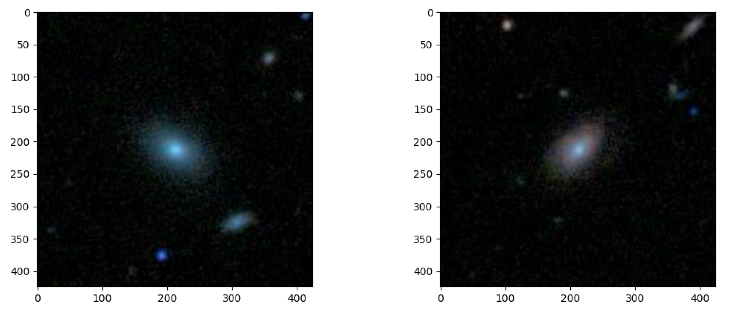
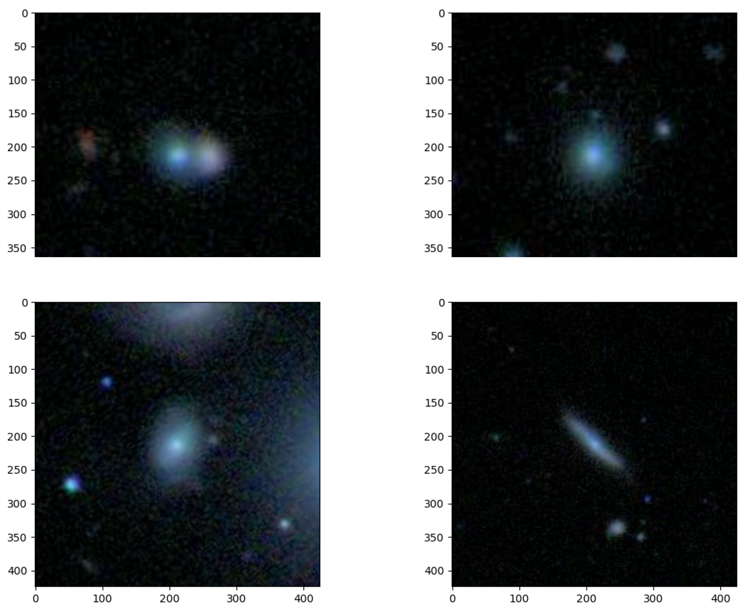
Figure 1 shows some examples of images from the GZ2 dataset. As mentioned, the diverse morphological characteristics of galaxies make their classification a complex task. The dataset includes an initial approximation of galaxy classifications, including around 150 distinct classes. However, this extensive classification scheme presents a challenge for machine learning algorithms to effectively train on. This is because of the increase in complexity as more classes are added and the problem becomes harder to solve due to imbalances in the size of each class. In order to obtain a more feasible training dataset while maintaining a relevant classification, Ref. [8] proposed a set of classes obtained from the following features:
  • t01_smooth _or_features_a01_smooth_weight ( p s m o o t h )—consistency-weighted number of votes for the “smooth” shape
  • t07_rounded_a16_completely_round_weight ( p c o m p l e t e l y r o u n d )—consistency-weighted number of votes for the “smooth and completely round” shapes
  • t07_rounded_a17_in_between_weight ( p i n b e t w e e n )—consistency-weighted number of votes for the “smooth and in-between roundness” shapes
  • t07_rounded_a18_cigar_shaped_weight ( p c i g a r s h a p e d )—consistency-weighted number of votes for the “smooth and cigar-shaped” shapes
  • t01_smooth_or_features_a02_features_or_disk_weight ( p f e a t u r e s / d i s k )—consistency-weighted number of votes for the “features or disk” shape
  • t02_edgeon_a04_yes_weight ( p e d g e o n , y e s )—consistency-weighted number of votes for the “edge-on” shape
  • t02_edgeon_a05_no_weight ( p e d g e o n , n o )—consistency-weighted number of votes for the “not edge-on” shape
  • t04_spiral_a08_spiral_weight ( p s p i r a l , y e s )—consistency-weighted number of votes for the “spiral structure” shape.
In the end, we obtained 5 classes instead of the original 150: completely round smooth, in-between smooth (between completely round and cigar-shaped), cigar-shaped smooth, edge-on, and spiral. The classes were ordered from 0 to 4 and Table 1 provides an overview of their properties and the number of samples.
Table 1 presents the features in the data file used during the labeling process. The values from the data file attributed to each of these properties are approximations made by the scientific community relating to each image in the GZ2 dataset.
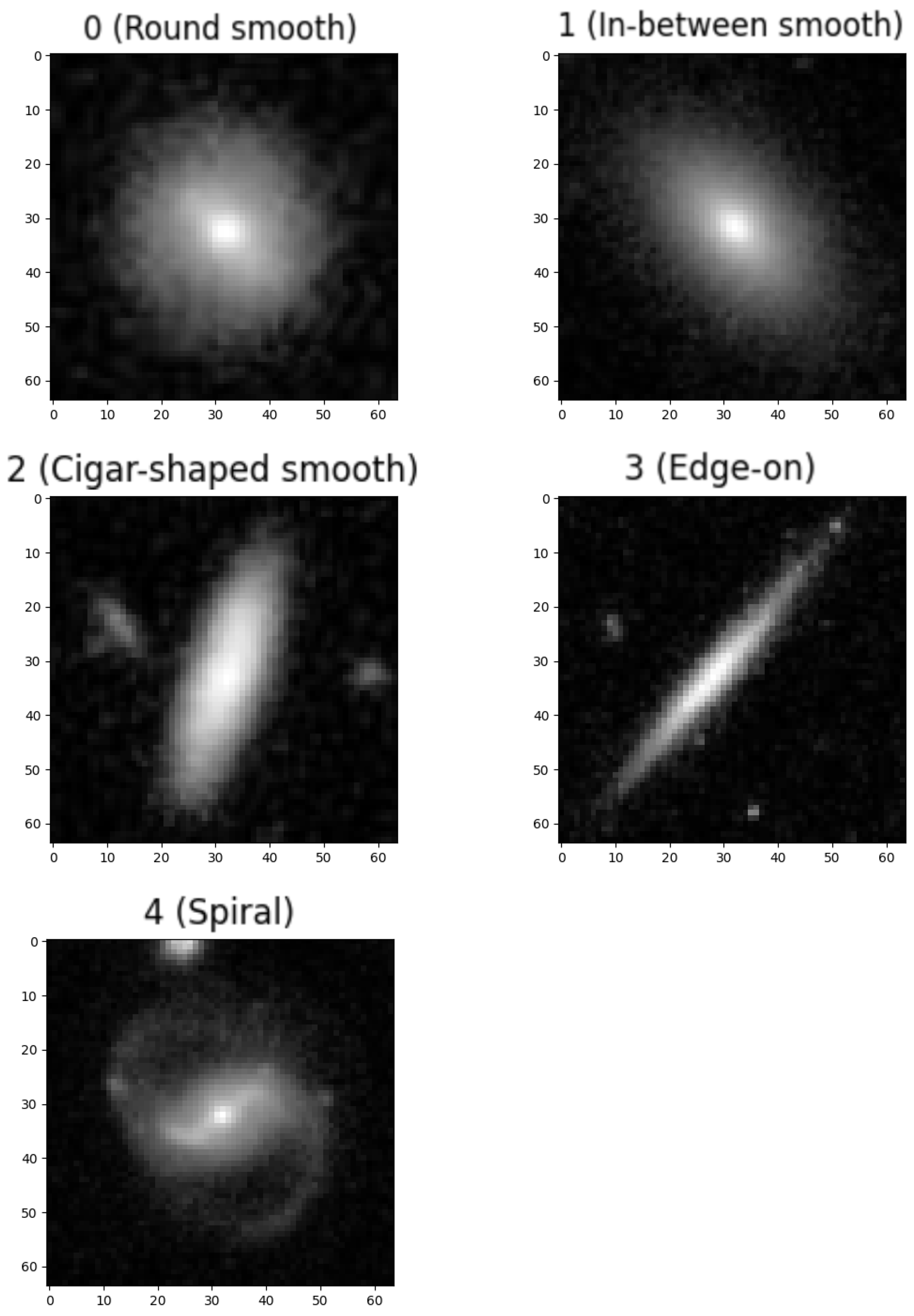
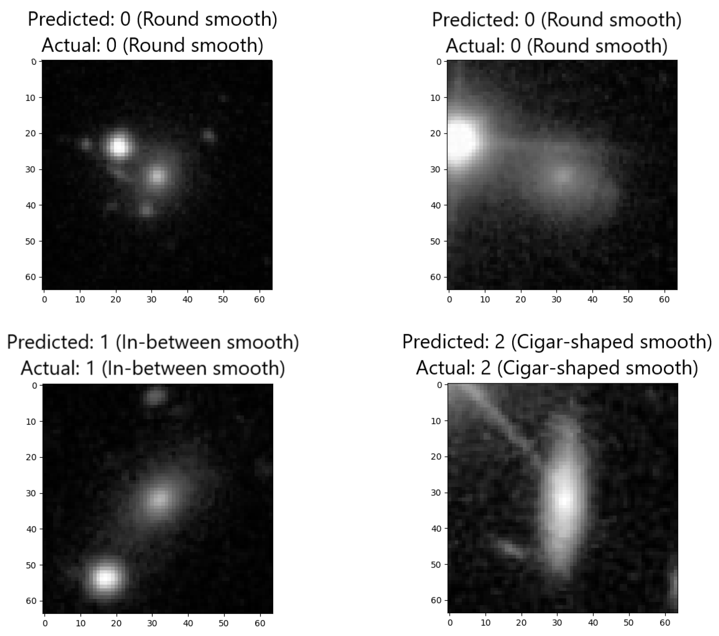
Figure 2 provides examples for each class. In total, 10,000 galaxy images were selected, and after applying the augmentation process, a total of 120,000 images were used for training our model. This process is presented in Section 3.3. The obtained dataset was randomly split into training, validation, and testing images, following a 75:15:10% split. This results in a total number of 90,000 training, 18,000 validation, and 12,000 test images.
In Table 2, the distribution of images is presented from a class perspective. In this table, a class imbalance can be observed, mainly related to classes 2 and 3, where the number of images represents 11.6% and 3.9%, respectively, out of the total number of images. The third row from Table 2 representing the test data will be used for most of the results and metrics presented in the paper.

3. Preprocessing

Image preprocessing algorithms and techniques are used to minimize training overfit while improving results. A small number of training images and low-class diversity can lead to overfitting. This means that the neural network learns to predict similar cases with high accuracy while underperforming on a completely new dataset.

3.1. Filters and Normalization

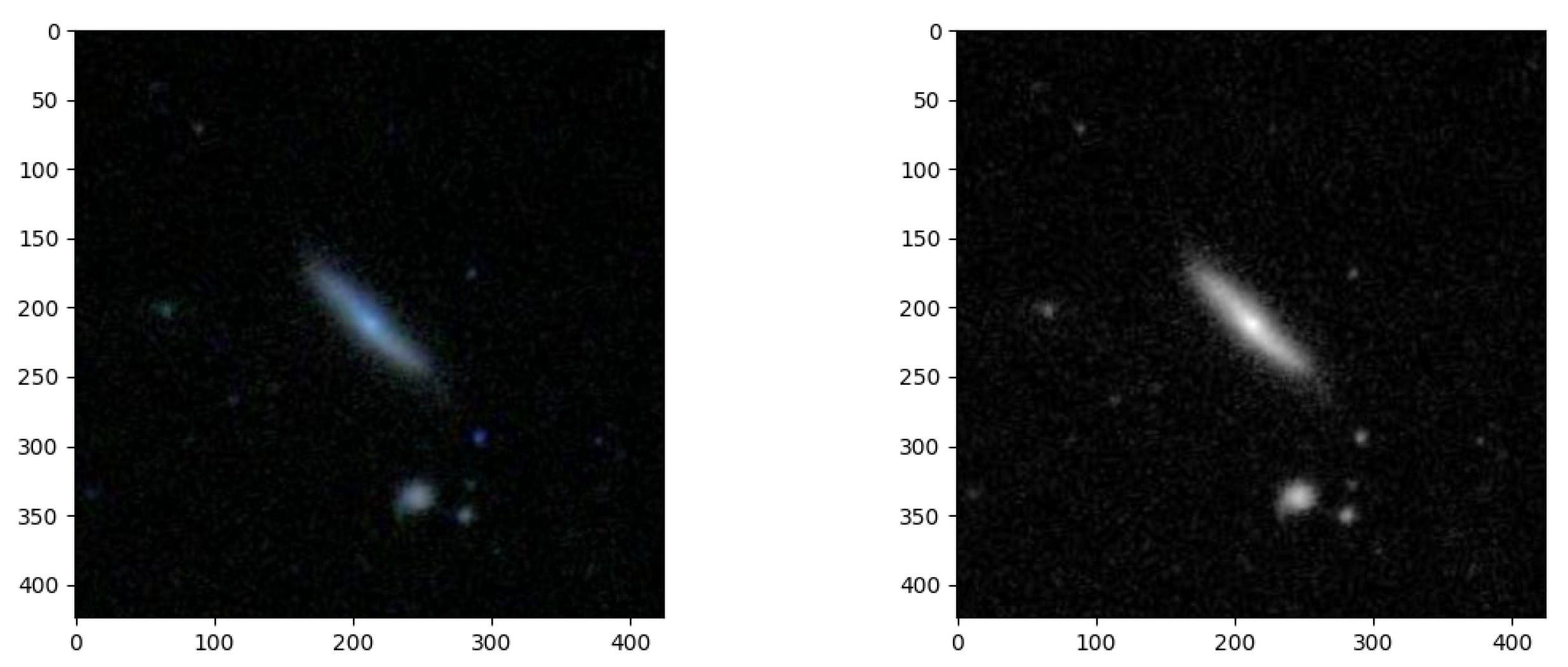
The first filter applied to the images is the grayscale transformation cf. Equation (1). This reduces the number of channels in the images from three to one. After this process, the image size becomes 414 × 414 instead of 414 × 414 × 3, thus reducing the computational complexity. This also improves the learning capabilities of the network, reducing the problem size as it also reduces the number of features the model needs to evaluate, thus reducing the overfit.
f ( R i , G i , B i ) = 0.299 · R i + 0.587 · G i + 0.114 · B i
where f ( R i , G i , B i ) is the resulting grayscale value of pixel i and Red, Green, and Blue are the pixel values of their corresponding channels. The coefficients 0.299, 0.587, and 0.114 correspond to the luminance-preserving weights for each channel, approximating the human perception of brightness [27].
Similarly, the normalization process helps by mapping the pixel values from [0, 255] to [0, 1], achieving numerical stability, improving convergence during training, and ensuring that all features have a similar scale. The equation to convert them to the unit interval is as simple as presented in Equation (2).
f ( x i ) = x i 255
where x i is the value of the current pixel.
Grayscaling and normalization improve the accuracy of our model by 10 % at the same time, reducing overfit.

3.2. Cropping and Scaling

The GZ2 dataset images are composed of deep space in large fields of view with the galaxy positioned roughly in the center. This leads to a significant amount of other information (noise) present in each image. This can be observed in Figure 1 and Figure 3.
To improve the classification accuracy, we need to reduce the background noise as much as possible. Some examples of noise are stars, other galaxies, and artifacts. These types of noise can be also observed in Figure 3, mostly below the central galaxy.
To reduce the noise, a crop from the center point of the image [212, 212] is employed. This crop has a size of 180 × 180 pixels from the image center. This value was obtained through testing a set of different crop sizes, starting from a size of 300 × 300 pixels. Through observations, the lowest crop size achieved performed best in the training process. This aided the decision to pick the minimum crop size in order to not cut information out of the centered galaxy, hence possibly reducing the network’s accuracy. Following a series of experiments, the crop size of 180 × 180 pixels was determined to be the minimum possible dimension in order to not cut any of the pixels contained within the galaxies. It also provided the best accuracy in our experiments compared with the other crop sizes tested. The crop is further down-scaled to a value of 64 × 64 pixels to reduce the information within the image and make the training process less likely to overfit by encouraging the network to focus on the center of the image. The process of down-scaling the image to 64 × 64 pixels from the cropped version of 180 × 180 pixels does not affect the information contained within the image; it just reduces the number of pixels the network uses for learning. Reducing this number helps the model focus more on the central point of the images, which is the galaxy. As a side effect of this down-scaling, the time needed for training is reduced as well.
Figure 4 presents the resulting image after the cropping and scaling process. It shows how much background noise was removed in this step, making the image ready for the next processing step.

3.3. Augmentation

The next step in image preprocessing is to augment the dataset with additional images. Augmentation is a technique used in machine learning when the neural network has to work with a limited dataset, and it helps to generate additional training data from the existing set by providing different views of the same data.
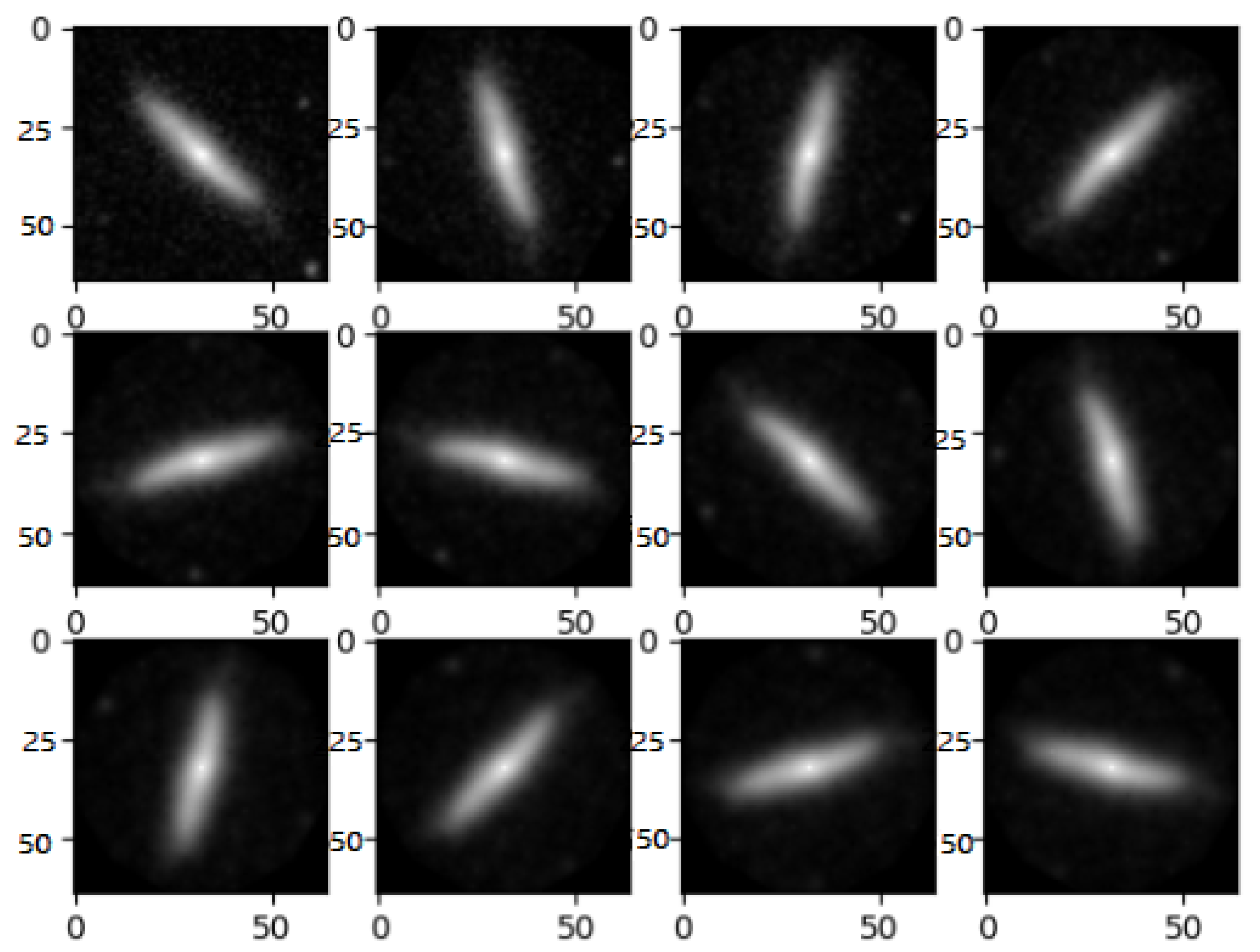
We extend the dataset by generating 12 times the number of images by applying an image rotation technique. This technique rotates the image by 30° 11 times clockwise. The same process but with different types of rotation can be observed in other papers as well. For example, Ref. [20] proposes a rotation of only four times. The formula for the rotation used is presented in [28].
Other processing filters and transformations available for augmentations include the following:
  • Flipping: Can be performed horizontally or vertically;
  • Median filtering: Helps with smoothing the image;
  • Gaussian or salt-and-pepper filtering: Can be used for adding noise.
These methods aim to reduce overfit and provide a richer training set for the neural networks. However, if the original data are not diverse enough, it can contribute to error propagation. For example, the top left image in Figure 4 contains another notable galaxy beneath. This can cause the algorithm to treat it as a feature for the training process and look for other images containing the same type of neighboring galaxies. If all 10,000 training images contain the same type of artifacts, rotating them 11 times, as seen in Figure 5 will give us 120,000 images that will be used to train a network that is unable to make accurate classifications on artifact-free images. For this reason, we decided to ignore flipping, median filtering, and Gaussian filtering methods.

4. Neural Network

As mentioned, our proposed solution is based on the CNN [29] and works by using convolutional layers to automatically learn and extract features from input images. These convolutional layers consist of small learnable filters (kernels) that slide across the input image, performing element-wise multiplications and summations to detect patterns and features at different scales.

4.1. Network Architecture

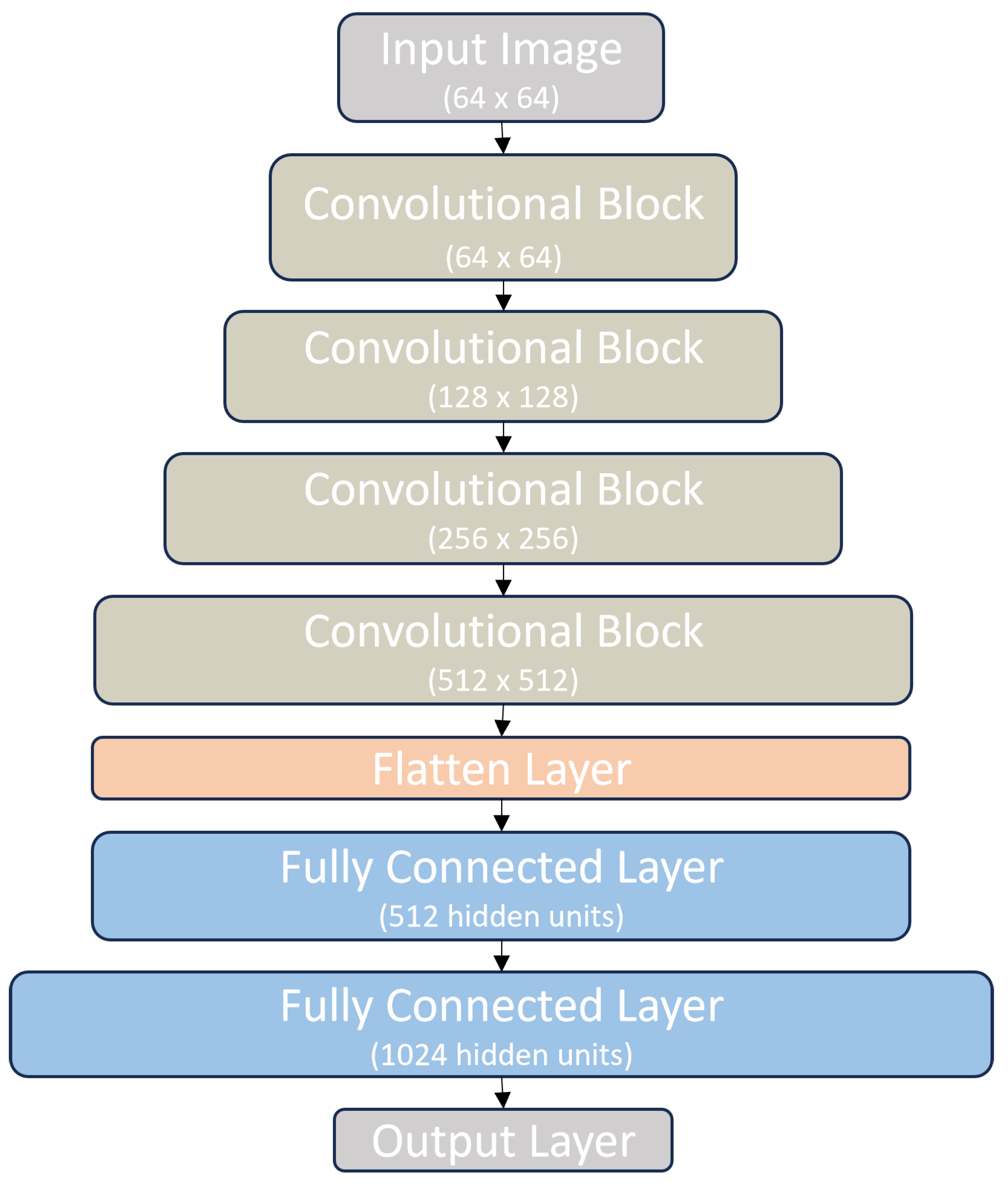
The network’s model architecture is organized into distinct blocks (or layers), starting with the Input Layer. This initial layer is designed to receive grayscale images of size 1 × 64 × 64.
The core of the model consists of Convolutional Layers arranged in four consecutive blocks. Each block encompasses several key components. The Convolutional Layers utilize convolution operations with varying numbers of filters and the same padding. The first block employs 64 filters of size 3 × 3, with subsequent blocks increasing the filter count to 128, 256, and 512, respectively. Following each Convolutional Layer, Batch Normalization is applied to enhance training stability. Activation functions introduce non-linearity, and max-pooling layers reduce spatial dimensions by a factor of two to enhance feature extraction. A popular choice for such an activation function is the Rectified Linear Unit (ReLU). It is obtained by choosing the maximum value between zero and the input value. An output is equal to zero when the input value is negative and the input value when the input is positive.
A Flatten Layer follows the Convolutional Layers, reshaping the 3D feature maps into a 1D vector, preparing the data for the Fully Connected Layers. The Fully Connected Layers are mainly comprised of hidden units. They refer to the individual neurons or nodes within these layers. These units receive input from all the neurons in the previous layer and contribute to the generation of the layer’s output. The Fully Connected Layers encompass two key components. The first Fully Connected Layer (Dense) consists of 512 hidden units, with Batch Normalization for stability, ReLU Activation functions for non-linearity, and a dropout mechanism (rate of 20%) to prevent overfitting. The second Fully Connected Layer has 1024 hidden units and follows a similar pattern, including Batch Normalization, ReLU Activation, and dropout with a rate of 50% to mitigate overfitting. This dropout percentage was obtained through trial and error, observing that a higher value on the second Fully Connected Layer obtained better results. The tested values for dropout were within [0, 80]%.
The architecture concludes with the Output Layer, configured based on the number of classes. It uses softmax as an activation function, resulting in a confidence score for each of the classes trained on. The final result is the class with the highest confidence score. The architecture previously described is present in Figure 6.

4.2. Hyperparameter Tuning

Within the network architecture are some outstanding hyperparameters. For the proposed network, these are the dropout rate, activation functions, batch normalization, pooling size, and padding. The dropout rate is the proportion of neurons to be randomly deleted during training to prevent overfitting. The dropout rate is employed in the proposed network at the fully connected layers level. The values used are of 20% after the first connected layer and 50% after the second fully connected layer.
There are several activation functions; some of the ones proposed in the literature are ReLU, sigmoid, softmax, and tanh. For the proposed network, ReLU is used for all of the convolutional and fully connected layers, while softmax is employed for the output layer. The choice of softmax as an activation function is for turning raw scores into probabilities, ensuring clarity in predictions and facilitating efficient optimization, especially in scenarios where classes are mutually exclusive. This technique is presented in [30]. Other layers use ReLU because of its efficiency in introducing non-linearity to enable better model learning by keeping positive values unchanged and suppressing negative ones.
Batch normalization operates by normalizing the values after the activation functions within subsets of data during training. The concept was introduced by Ioffe in [31]. Batch normalization helps mitigate issues like vanishing or exploding gradients, enabling faster and more stable convergence during training. The key idea behind batch normalization is to normalize the mean and standard deviation (SD) of each channel within a subset from the data.
Pooling is a down-sampling technique used to reduce the spatial dimensions of feature maps in a CNN. The size used in this architecture is 2 × 2 for the convolutional blocks.
Padding is a technique used to control the spatial dimensions of feature maps after pooling operations. It involves adding extra values (usually zeros) around the edges of the input data or feature maps. Padding serves two primary purposes: maintaining spatial dimensions and preventing the loss of information near the edges. There are two common types of padding: “valid” (no padding) and “same” (adding padding to maintain the output size). The proposed architecture uses the latter one.
The proposed model was implemented and trained using Python 3.9 and TensorFlow 2.14 with CUDA GPU support. The process of hyperparameter tuning involves adjusting certain parameters to better suit the galaxy classification task, making learning more efficient. These parameters can be embedded within the architecture itself or they can be used to enhance the training process. Some examples of hyperparameters used in the training process of the proposed network are epochs, learning rate, batch size, optimizer [32], loss function, dropout rate [33], activation functions [34], batch normalization [35], pooling size [36], and padding [29]. While the first five hyperparameters improve the training process, the last five help in creating a more suitable architecture for the problem of classification.
The epochs parameter refers to the number of complete passes through the training dataset during training and affects the model convergence. The learning rate is a small positive value that determines the step size when updating model weights during training. It is a critical hyperparameter for optimization algorithms like gradient descent. Batch size refers to the number of training examples used in each iteration of training. It impacts memory usage and the speed of convergence. The optimizer and loss function work together to minimize the error. There are multiple types of optimizers: stochastic gradient descend [37], RMSprop [38], and Adaptive Moment Estimation (Adam). According to [32], the Adam optimizer was developed for large datasets and multi-class classification problems and is the one we also employ for our network architecture. The loss function quantifies how well the model is performing. Optimizers search for the parameter values minimizing the loss value, effectively making the model’s predictions as accurate as possible.
The Adam optimizer maintains both the first and second moments of the gradients and employs adaptive learning rates for each parameter. This dynamic learning rate adjustment makes it effective in training deep networks, as it adapts to the individual gradients of each parameter, resulting in faster convergence and improved performance. Adam is known for its robustness, quick convergence, and suitability for a wide range of deep learning tasks, making it a popular choice in machine learning research and applications.
Early stopping monitors a model’s performance during training and stops training when no improvement on unseen data is observed, thus preventing loss. This means that each model is trained on a different number of epochs until it obtains the best results. In order to configure early stopping to work properly with our problem, we used the following parameters:
  • monitor with a value of ‘val_loss’: Tells the process to watch the validation loss. Validation loss is how well your model performs on unseen data, which helps identify overfitting.
  • min_delta with a value 0: This sets the minimum amount the validation loss needs to improve to be considered progress.
  • patience with a value of 2: This is the number of epochs the model will wait without an improvement in validation loss before stopping training.
  • mode with ‘auto’ value: This tells the process to automatically choose between ‘min’ (looking for the lowest validation loss) or ‘max’ (looking for the highest validation metric), depending on the metric being monitored (in this case, ‘val_loss’, so it will look for the minimum).
While there are some fixed parameters for multi-class classification problems, such as the loss function or optimizer, there are others that can be adjusted to provide better results in the training process. The hyperparameters tested with different values are the learning rate, epoch, and batch size. The following results are obtained by training the proposed network over a period of 12 epochs. In order to obtain this value of 12 epochs, we employed the early stopping technique.
Table 3 shows how the training is impacted by the different values of the learning rate. The best two identified are 0.001 followed by 0.0001, which provide acceptable results. As observed, as the learning rate increases, the worse the results become. This happens because the learning rate adjusts the weights either by a too-large or a too-small step. This complicates the process of obtaining the desired weights, as either the step is significantly different or the adjustment is too little, leading to the requirement of an excessive number of steps.
If the learning rate and epochs are strongly correlated with the accuracy and precision of the network, the batch size is more related to the memory usage and speed of training. Different values provide little to no improvement, compared with the 16 batches model, in the accuracy, but increase the training time by more than 50%.
Table 4 depicts how a smaller batch size takes a significantly greater amount of time. This is paired with the idea of an accuracy increase, which is not happening for the first size of 8, compared with the next one. The second size of 16 not only performs quicker but is more accurate than it. As for the learning rate, the best values for batch sizes are somewhere in the middle, with a size of 16 being the best one, followed by a size of 32. In this case, the size-16 one was chosen, even with a compromise on the space and time aspects. As stated before, the improvements between the batch sizes are not outstanding. The preferable choice is the best one in terms of accuracy if the cost is not too great. For instance, in our case, the difference between the size-32 one and the size-16 one is 36% (about 1800 s) for just a 0.62% accuracy improvement. Even if the accuracy increase is not so great, the trade-off is only a training period increase of approximately 1800 s, which makes it worth it.

4.3. Loss Function

The loss metric represents the model’s error during training. It is computed using a loss function, such as categorical cross-entropy [39], and measures how well the predicted values align with the actual values. Lower loss values indicate better model performance.
The proposed model uses the categorical cross-entropy. This is a widely used loss function for multiclass classification tasks. It quantifies the dissimilarity between the predicted class probabilities and the actual class labels. The goal is to minimize this loss during training.
l o s s = i = 1 C y i · l o g ( p i )
where C represents the number of classes, yi is the actual (true) probability of the sample belonging to class i, and pi is the predicted probability of the sample belonging to class i.

4.4. Training Process

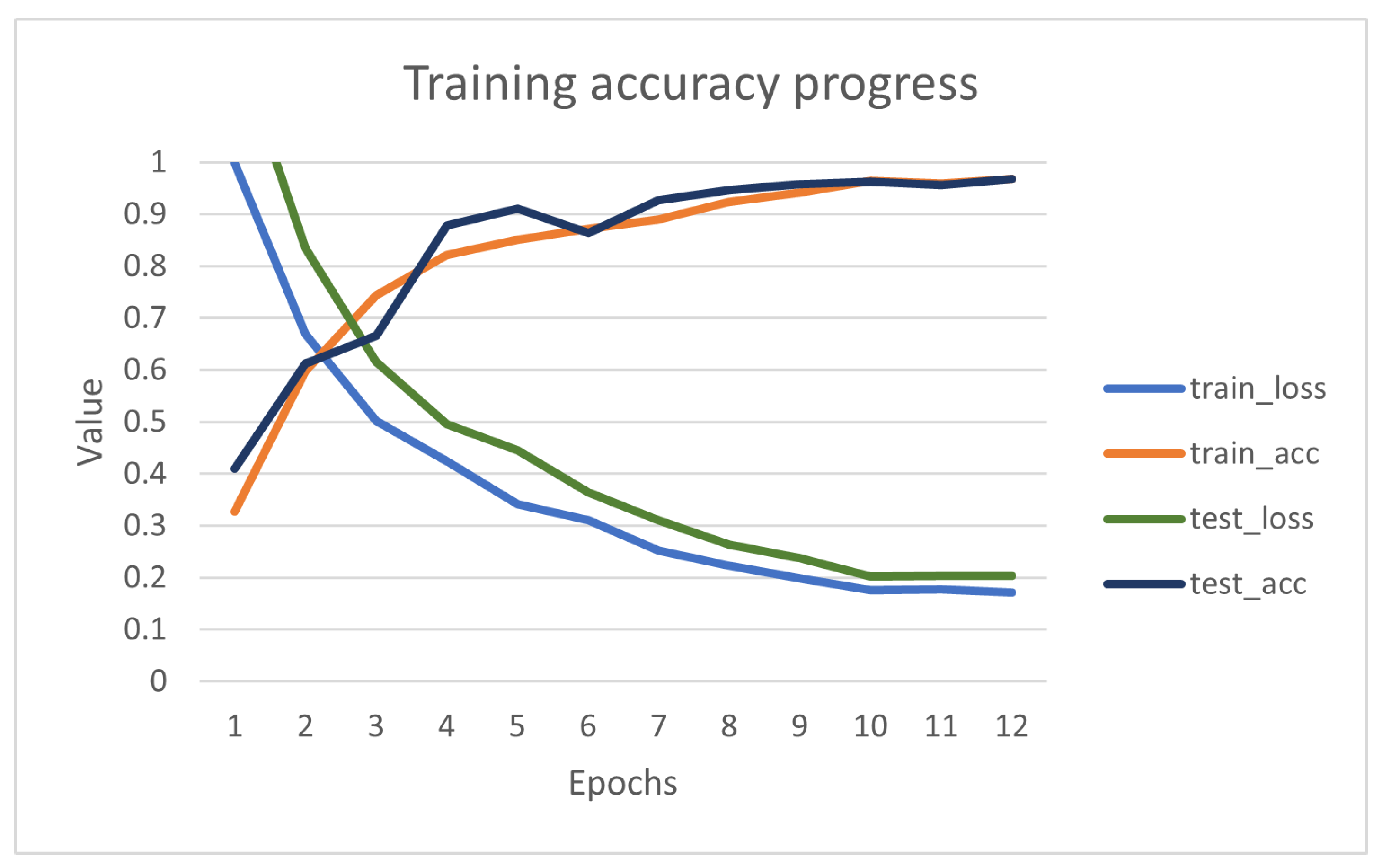
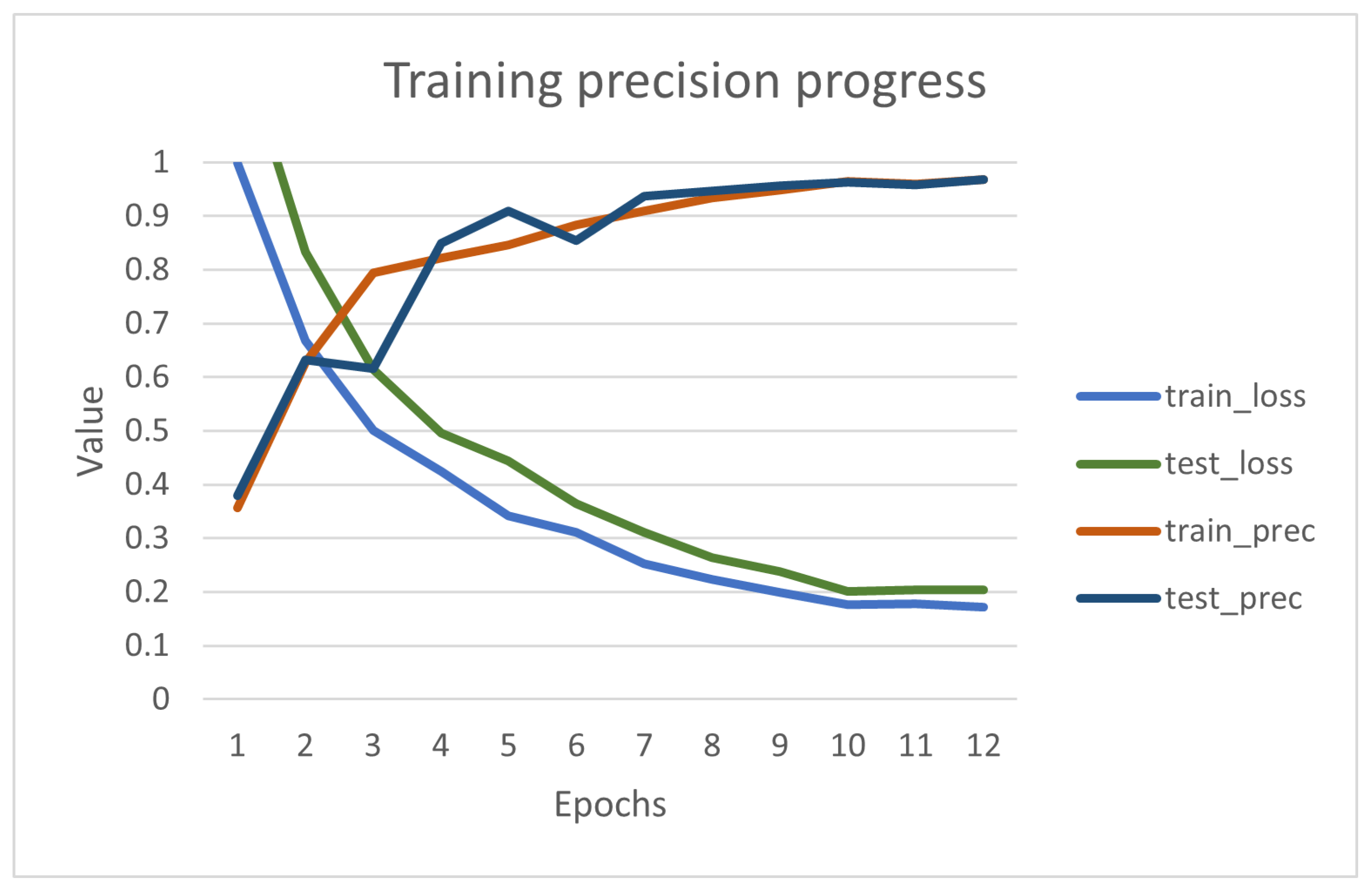
The relationship between the training achievements and the loss functions can be observed in Figure 7. In this figure, it is presented how the proposed model trained in regards to the accuracy, precision, and loss. In dark blue, we have the validation metric, orange represents the training value of the metric, and green and light blue represent the validation value of the loss and the training value of the loss, respectively. Starting with a low value for the metrics and a higher value for the loss functions, by training for 12 epochs, we achieve better results, with this progression slowing down after 4 or 5 epochs. During this training process, we also tried to increase the number of epochs to 15, 20, and 30, but all these versions of the network introduced overfit and resulted in a generally worse outcome, lowering the accuracy of the model.
Each epoch exhibits a steady improvement in the accuracy and precision, while the loss function is continuously reduced. The plot shows how, during the initial epoch, accuracy and precision had values of around 30%, i.e., as though the network were guessing one of the results based on its frequency. However, after training, these metrics increase to 96.83% and 96.75% for accuracy and precision, respectively. Furthermore, the low value of 0.1718 attributed to the loss function shows how close the predictions are to the correct labels.
The GitHub repository containing the code for the presented solution is open and available at https://github.com/raulurechiatu/deepskydetection/tree/galaxy_classification (accessed on 14 April 2024).

5. Results

In this section, we present the results of the proposed network. We use a variety of metrics: accuracy, precision, F1 score, confusion matrices, AUC, Receiver Operating Characteristic (ROC), and stochastic ordering. The results are compared with other state-of-the-art neural networks (i.e., ResNet-50, DenseNet, EfficientNet, Inception, and MobileNet), as well as more research on classifying galaxies [20].

5.1. Summary of Results

The comparison between the classes, as depicted in the confusion matrix from Table 5, provides a detailed look into the neural network’s performance across the distinct categories of classes. Notably, the matrix exhibits a strong diagonal pattern with bold values, representing correct predictions for each class. For Class 0, the model achieves 3472 correct predictions, making it the most accurately classified class. Similarly, Class 1 demonstrates high accuracy with 4878 correct predictions, indicating a model that effectively discerns instances from this category. Moving to Class 2, we find 1141 correct predictions, revealing the network’s capacity to accurately classify instances from this class. Despite being less frequent in the dataset, Classes 3 and 4 are also correctly identified with 439 and 1947 predictions, respectively. This confirms the model’s reliable performance across all classes, highlighting its strong multi-class classification capabilities.
To further analyze our class-based comparison, we randomly split our analysis into training and validation data subsets. This differentiation allows us to study how our CNN performs on individual classes during both the validation and testing phases. By evaluating the precision, recall, and F1 score for each class in these distinct datasets, we obtain valuable insights into the model’s ability to generalize its learning from the training set to previously unseen validation data. This partitioned examination enables a better understanding of performance across diverse classes and helps to optimize our model more efficiently.
To better understand the data behind these confusion matrices, in this section, we switch our focus to a class-based comparison of the results. This helps us to better understand how our neural network performs across individual classes. Through an examination of class-specific precision, recall, and F1 scores, we gain a better understanding of the model’s performance and the disparities among various categories.
The comparison between the classes in the multi-class classification problem, as shown in Table 6, reveals valuable information about the model’s performance across multiple categories. Notably, Class 1 stands out with an impressive accuracy rate of 99.03%, accompanied by precision and recall metrics at the same elevated level. This demonstrates the model’s remarkable consistency in accurately classifying instances from this category. This can also be correlated to the fact it has the biggest sample size. Similarly, Class 0 exhibits strong performance with an accuracy of 98.92%, indicating a high degree of precision and recall. This level of accuracy across two classes underlines the model’s reliability and accuracy in correctly identifying instances from these groups. As we progress to Class 2, an accuracy of 96.12% is maintained, accompanied by parallel precision and recall scores. This reflects the model’s proficiency in recognizing instances from Class 2, offering a robust multi-class classification solution. The results further demonstrate the model’s capability to handle Classes 3 and 4 with accuracy rates of 91.46% and 97.35%, respectively, and precision and recall metrics mirroring these percentages. These close values in performance showcase the model’s consistency in correctly categorizing instances from these classes, more so from the first two and the last one, making it a reliable classifier for this multi-class problem.
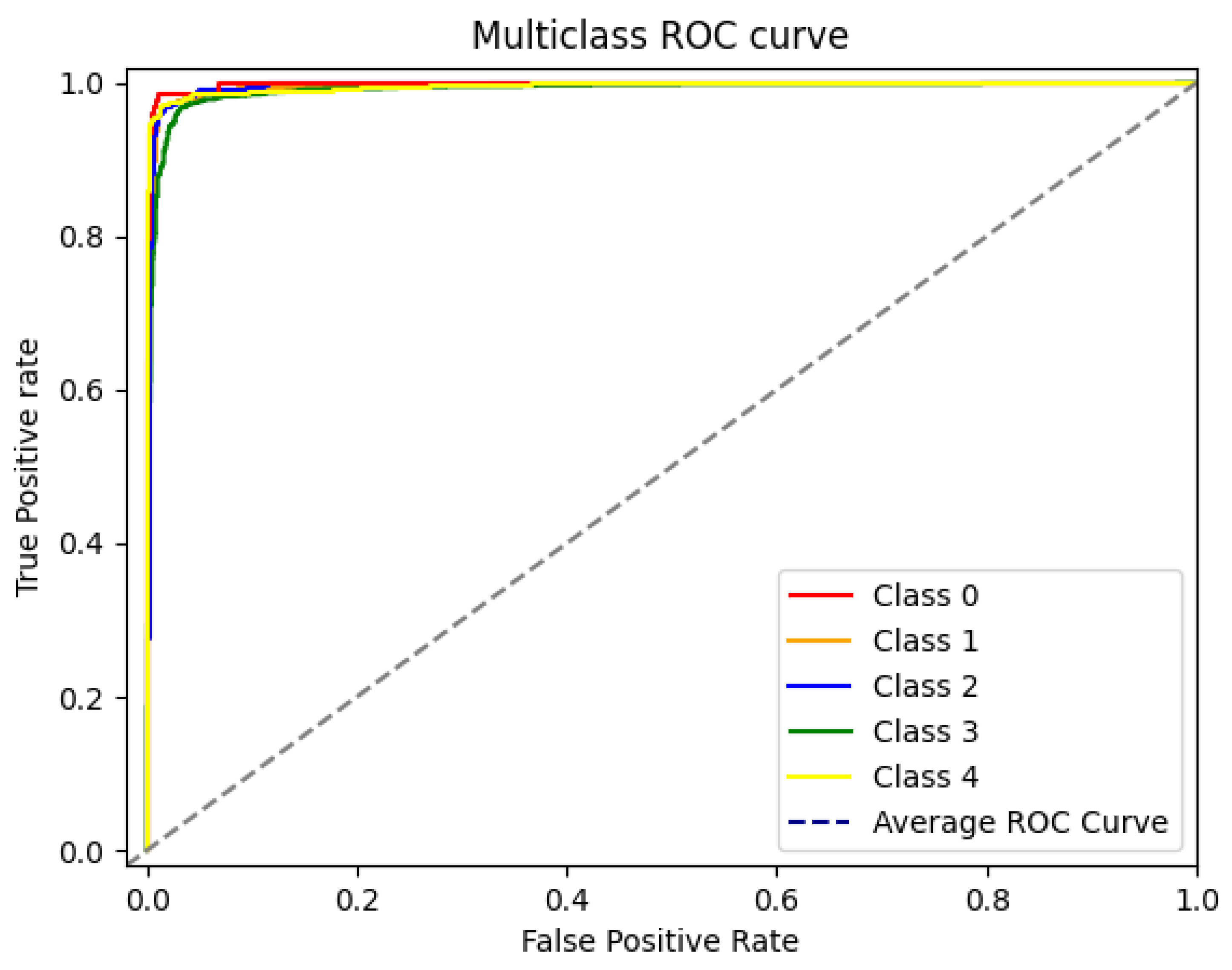
Figure 8 illustrates the ROC curve for our model’s classification of the five classes on the testing set. Each distinct color within the graph corresponds to a specific class. The proximity of the True Positive Rate (TPR) to 1 and the False Positive Rate (FPR) to 0, as evidenced by the ROC, showcases the performance of our model on each class. In essence, the closer the curve aligns with the upper-left corner, the more accurate the predictions. Cf. Figure 8, the ROC curve for each class exhibits good performance. Notably, the 1st class achieves the highest predictive accuracy, while the 3rd class lags slightly in performance, primarily attributed to the scarcity of available cigar-shaped images in the dataset. Furthermore, the average AUC for our model amounts to an impressive 0.9921, indicative of the model’s exceptional overall predictive capabilities. The diagonal line showcased in Figure 8 represents the performance of a random classifier.

5.2. Comparison with Other Methods

In this section, we compare the proposed architecture and its results with other CNNs and related works proposed in the literature, as mentioned earlier.
We must first understand the architecture and the main features of some state-of-the-art neural networks. The distinguishing feature of ResNet-50 [22] is the use of residual blocks. These blocks contain skip connections, or shortcuts, that allow the network to skip over one or more layers. This skip connection enables the network to learn residual functions, making it easier to train very deep networks. For DenseNet [23], these outstanding features are its densely connected layers. In traditional neural networks, each layer receives input only from the previous layer. In contrast, DenseNet connects each layer to all subsequent layers. This dense connectivity facilitates feature reuse and encourages gradient flow, making it easier to train very deep networks. The Inception architecture [21], also known as GoogleNet, introduces the concept of inception modules, which are building blocks for the network. These modules perform multiple convolutions of different kernel sizes (1 × 1, 3 × 3, 5 × 5) and max-pooling operations on the input data in parallel. The outputs of these operations are concatenated along the depth dimension, allowing the network to capture features at various scales. The core idea behind EfficientNet [24] is to achieve model scalability by uniformly scaling three critical dimensions of a CNN architecture: depth, width, and resolution. By systematically and uniformly scaling these dimensions, EfficientNet models maintain a balance between model capacity and computational efficiency. And, lastly, MobileNet [25] introduces a significant innovation in the use of depthwise separable convolutions, which replace traditional convolutions. Depthwise separable convolutions consist of two layers: depthwise convolutions (pointwise convolutions) and 1 × 1 pointwise convolutions. These layers are computationally more efficient than standard convolutions. Also, this network is a more lightweight version of neural networks compared with its previous counterparts.
It is important to note that these networks were trained with the same set of hyperparameters that the proposed network was trained on. These hyperparameters are a batch size of 16, a learning rate of 0.001, categorical cross-entropy as a loss function, and an Adam optimizer. Besides these parameters, in order to attain convergence on each of the trained networks, we used early stopping, as we did for the proposed network mentioned in Section 4.2.
Table 7 shows the comparison between the proposed network architecture and state-of-the-art counterparts previously described. It can be noticed that our designed CNN provides better results than the rest. The proposed CNN achieved a testing accuracy of 96.83%. This marked an improvement beyond the accuracy rates attained by the competitors, which hovered around 94% after the validation. This was also the case when compared with [20], which obtained an accuracy of 95.2% on a classification problem with the same number of five classes. Also, Ref. [19] have a good accuracy of 94.47%, with the main reason for a lower accuracy being the class imbalance present in it. This results in the fact that the proposed network was better at training on a limited number of images compared with the proposed research from Zhang.
Because of the class imbalance, cf. Table 6, under the sample size column, accuracy can be unreliable on its own. For this reason, other metrics such as precision, recall, and the F1 score can be helpful. If all these metrics give good results, we are looking at a general solution for our problem, whereas if these values are unsatisfactory, the model needs improvements. While precision is important when false positives need to be reduced, the recall is mostly used to evaluate the miss rate of true positive values. For the problem of class imbalance, the most important metric is the F1 score, as it allows for a comprehensive assessment of the model’s performance, taking both false positives and false negatives into account.
With values of 96.75%, 96.52%, and 96.72% for precision, recall, and the F1 score, our proposed CNN provides a better solution to the problem of galaxy classification. This can be observed in the comparison with other networks, where most of them obtained values of around 94%, as well as the architecture proposed by [20], which provided values of 95.12%, 95.21% and 95.15% for precision, recall, and the F1 score.
Another comparison can be made when we inspect the number of nodes of each network. In this comparison, we do not see a big difference between the proposed network and the state-of-the-art ones. The fact that the number of features is similar to theirs while achieving higher accuracy suggests that the layers used are more suitable for the suggested problem.
These features are represented by the total number of neurons in the fully connected layers of this neural network; the number of units in these layers can be added up, and the results are represented in Table 8.
The performance of our network is also validated by the lower values obtained by the loss function. Table 7 summarizes the results. Achieving the lowest value of the tested networks suggests that the results that were predicted by the proposed network are closest to the truth. Achieving a difference of around 0.04 from the best performer, DenseNet obtained a loss value of 0.2174.
Accuracy and loss are inversely correlated. As accuracy increases, loss decreases. As the model becomes better at minimizing the error represented by the loss function, its accuracy increases. The proposed architecture achieved a remarkable accuracy of 96.83%, with a very low loss of 0.1718. This indicates that the model excels at correctly classifying galaxies and does so with high confidence, compared with the other solutions peaking at 95.20% accuracy with a slightly higher loss of 0.1908. All the training of the state-of-the-art networks is conducted using early stopping, achieving their convergence. While the other models perform well, they have a lower accuracy compared with the proposed model, and the loss indicates slightly less precise class predictions.
Evaluating the performance of CNNs often means relying on point estimates like accuracy or loss. However, these metrics might not fully capture all the properties of CNNs, particularly when dealing with tasks involving uncertainty or risk. In [40], the authors leverage the concept of stochastic ordering to provide a comprehensive comparison of neural networks. Similarly, we compare the proposed network architecture against established state-of-the-art models in the following paragraphs. Stochastic ordering allows us to assess which model offers a more favorable distribution of outcomes for the task at hand. This approach goes beyond traditional point estimates and provides valuable insights into the relative risk profiles and potential benefits of each tested architecture.
We applied this technique on our proposed network’s and established architectures (ResNet-50, DenseNet, Inception, EfficientNet, MobileNet). We leveraged the GZ2 dataset, randomly selecting 4511 images for evaluation. For each image, all six networks provided a prediction confidence value between 0 and 1. For each image, the statewise dominant is chosen based on the network that predicted the correct class with the highest confidence value. In stochastic ordering, a statewise dominant variable guarantees at least equal or better results compared with all others, with at least one scenario offering a strictly better outcome. This approach allowed us to analyze the distribution of confidence scores across the entire dataset. Also, this provides insights into which network consistently produces not only accurate classifications but also the most reliable confidence estimates for the task of galaxy morphology classification in the GZ2 dataset. Based on this stochastic ordering, other metrics are computed to further the understanding of the network’s performance. These metrics are the confidence mean, median, SD, and variation.
The proposed network demonstrates the highest count of dominant instances, with a total number of 2465 samples having the best confidence. This is more than half of the 4511 evaluated images, making it the “stochastic dominant”. This indicates that the network’s predictions were not only precise, but also the most confident (with the highest score) for a significant portion of the dataset in comparison to other models.
The proposed network also presents the highest average and median confidence with values of 0.9457 and 0.9992. This suggests a strong tendency to be highly confident in its classifications. The SD and coefficient of variation for the proposed network’s confidence scores also have the lowest values of 0.1129 and 0.0127. This shows a more consistent level of confidence across its predictions compared with other models.
An interesting event to be observed happens between the ResNet-50 and DenseNet networks. In Table 9, even if the DenseNet architecture obtained more dominant instances, all the other metrics indicate that ResNet-50 is more reliable and consistent. This tells us that the ResNet-50 architecture is more confident and robust in its predictions, but DenseNet is a better network for a large number of detections.
According to the stochastic ordering analysis, the proposed network shows strong performance in categorizing galaxy morphology. It has a high frequency of dominant instances, indicating that its predictions are often the most confident and precise. Furthermore, the reduced variability in confidence scores suggests a consistent level of reliability in the network’s outputs.

5.3. Examples

To better showcase the results obtained by the proposed neural network, this section presents some prediction examples for the multi-class classification problem. This section also contains a comprehensive display of image examples representing all five distinct classes. The examples, analyzed and predicted by the proposed neural network, offer a visual aid to better asses the model’s strengths and weaknesses. They provide a visual understanding of its ability to discern and categorize various objects, patterns, or entities and showcase the challenges of the dataset itself.
Among the predictions generated by our CNN, there exist instances that pose unique challenges due to the presence of artifacts or complexities within the images, cf. Figure 9. These difficult, yet ultimately correct predictions showcase the model’s ability to understand subtle details and overcome visual challenges found in multi-class classification. In the face of artifacts, noise, or strange patterns that may confuse other systems, our neural network showcases its accuracy and adaptability. These successful classifications provide proof of the network’s robustness and its capacity to make well-informed decisions even when faced with challenging real-world data. Such capabilities are mandatory in applications where image quality and content can vary widely and where the presence of artifacts is a common occurrence. These challenging but accurate predictions exemplify the neural network’s potential to contribute to the advancement of various domains by providing reliable multi-class categorization, even in the presence of complex image artifacts.
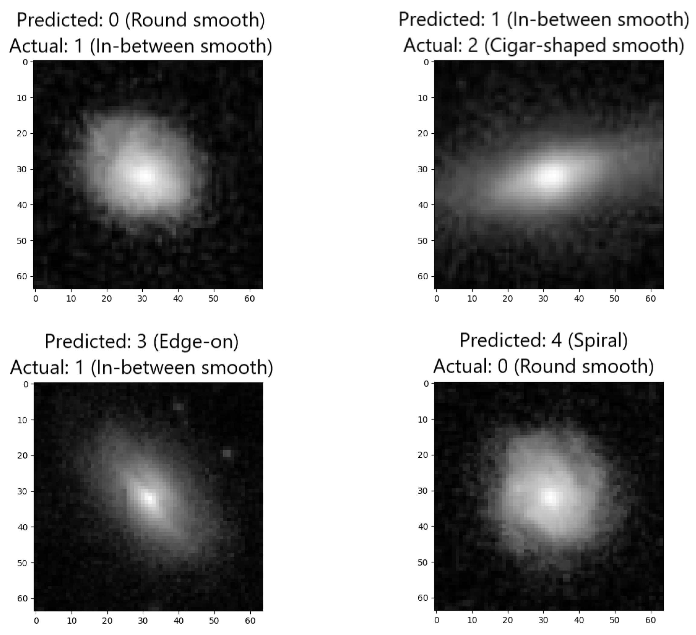
While the performance is satisfactory, occasional predictions were missed, as presented in Figure 10. These instances, where the model assigns an incorrect label, provide insights into the boundaries of its capabilities and the complexity of real-world data. These missed predictions may appear due to complex image content, ambiguous patterns, or unexpected variations within the dataset. While they underscore the challenges associated with multi-class classification, they also drive us to continually refine and optimize the model. Understanding the nature of these missed predictions serves as valuable information for model improvement and fine-tuning. By addressing the details and complexities that lead to these cases, we aim to enhance the network’s robustness and further its potential in applications where precision and accuracy are key factors. These missed predictions remind us of the ongoing process to advance and better the state of the proposed network, promoting the development of more intelligent and adaptable neural networks.
To further evaluate the effectiveness of our proposed algorithm, we applied it to a set of 50 galaxy images obtained from the James Webb Space Telescope (JWST)’s deep field observations. By testing our algorithm on this challenging dataset containing previously unseen and potentially unique galaxy morphologies, we can assess its robustness and generalizability to a wider range of astronomical objects, compared with traditional datasets.
In [41], the process used to obtain JWST’s images is explained. They are taken using various infrared filters and then combined. JWST utilizes its infrared cameras to acquire multiple grayscale intensity images. These images correspond to distinct wavelengths of infrared light, invisible to the human eye, captured through a set of six specialized filters. Following data acquisition, scientists assign a corresponding visible color to each filter’s dataset. The longest wavelengths are mapped to red, while the shortest wavelengths are assigned blue, with intermediate wavelengths represented by a spectrum of intervening colors. Finally, by combining these color-coded images, a composite image is produced, revealing the full spectrum of color observed in the now-famous astronomical photographs.
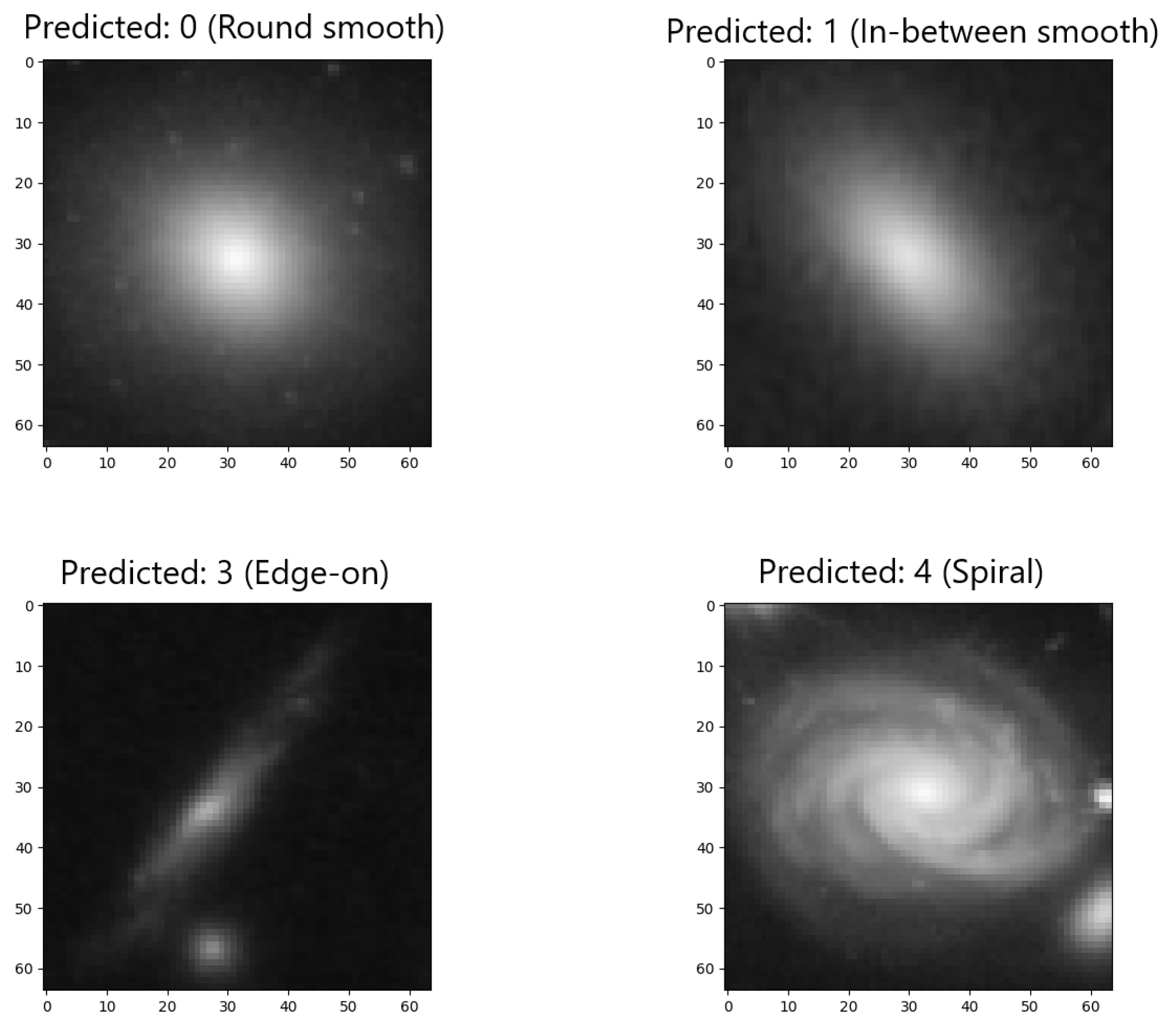
To prepare the data for analysis with our proposed algorithm, individual galaxies were extracted from the deep field image. Following extraction, each galaxy was cropped to isolate the object of interest. Finally, the cropped images were resized to a standardized size of 64 × 64 pixels and converted to a grayscale format to ensure compatibility with our model’s input requirements. The resulted images and the predictions of the network can be observed in Figure 11.
6. Summary and Conclusions

The problem of morphological galaxy classification is a topic that continues to evolve as richer and more diverse surveys are performed and fine-tuned neural networks are designed and trained. One example is the James Webb space telescope, which will provide many new images of deep fields never before seen, not necessarily with completely new data, but with much more and diverse data, hence the need to automate the classification of these galaxies, as it is an impossible task for astronomers with the current instruments.
In this paper, we presented a novel solution for classifying the morphology of galaxies. The proposed algorithm uses machine learning and trains a CNN to achieve the aim. The data are classified into five classes [8]: completely round and smooth, in-between smooth, cigar-shaped smooth, angular, and spiral. The dataset used to train the network is GZ2, which contains 243,434 images. The size of the images is 414 × 414× 3 pixels. In the preprocessing phase, filters, normalization, cropping, scaling, and magnification are used. A 64 × 64 × 1 image is created from the images, centered on the galaxy in the middle of the image.
The proposed network achieves accuracy rates of 96.83% and precision rates of 96.75%. These rates are beyond some existing solutions in the literature, such as that of [20], which achieve rates of 95.2% accuracy. Compared with some state-of-the-art networks, the proposed one performed better in terms of accuracy. Networks such as ResNet-50, DenseNet, EfficientNet, Inception, and MobileNet achieved accuracy rates between 92% and 95%.
The current model relies solely on pixel information that the CNN can extract without performing additional operations, such as the predicted class or other morphology-related values of the image. While it has proven to be efficient at classifying galaxies, there is still room for improvement, and the introduction of additional information is planned for the future. Another approach is to use an ensemble model consisting of our model and other current models such as ResNet-50, DenseNet, EfficientNet, Inception, or MobileNet, as this may be a way to improve the classification algorithm.

Author Contributions

Conceptualization, R.U. and M.F.; Methodology, R.U. and M.F.; Software, R.U.; Validation, M.F.; Formal analysis, R.U.; Data curation, R.U.; Writing—original draft, R.U.; Writing—review & editing, R.U. and M.F.; Visualization, R.U. and M.F.; Supervision, M.F.; Project administration, M.F. All authors have read and agreed to the published version of the manuscript.

Funding

This research received no external funding.

Data Availability Statement

Data available within the article.

Conflicts of Interest

The authors declare no conflict of interest.

References

  1. Hubble, E.P. Extragalactic nebulae. Astrophys. J. 1926, 64, 321–369. [Google Scholar] [CrossRef]
  2. Sandage, A. The Classification of Galaxies: Early History and Ongoing Developments. Annu. Rev. Astron. Astrophys. 2005, 43, 581–624. [Google Scholar] [CrossRef]
  3. Mezcua, M.; Farrell, S.; Gladstone, J.; Lobanov, A. Milliarcsec-scale radio emission of ultraluminous X-ray sources: Steady jet emission from an intermediate-mass black hole? Mon. Not. R. Astron. Soc. 2013, 436, 1546–1554. [Google Scholar] [CrossRef]
  4. Dey, A.; Schlegel, D.J.; Lang, D.; Blum, R.; Burleigh, K.; Fan, X.; Findlay, J.R.; Finkbeiner, D.; Herrera, D.; Juneau, S.; et al. Overview of the DESI Legacy Imaging Surveys. Astron. J. 2019, 157, 168. [Google Scholar] [CrossRef]
  5. Chambers, K.C.; Magnier, E.A.; Metcalfe, N.; Flewelling, H.A.; Huber, M.E.; Waters, C.Z.; Denneau, L.; Draper, P.W.; Farrow, D.; Finkbeiner, D.P.; et al. The Pan-STARRS1 Surveys. arXiv 2016, arXiv:1612.05560. [Google Scholar] [CrossRef]
  6. Labbé, I.; van Dokkum, P.; Nelson, E.; Bezanson, R.; Suess, K.A.; Leja, J.; Brammer, G.; Whitaker, K.; Mathews, E.; Stefanon, M.; et al. A population of red candidate massive galaxies ~600 Myr after the Big Bang. Nature 2023, 616, 266–269. [Google Scholar] [CrossRef]
  7. Lintott, C.J.; Schawinski, K.; Slosar, A.; Land, K.; Bamford, S.; Thomas, D.; Raddick, M.J.; Nichol, R.C.; Szalay, A.; Andreescu, D.; et al. Galaxy Zoo: Morphologies derived from visual inspection of galaxies from the Sloan Digital Sky Survey. Mon. Not. R. Astron. Soc. 2008, 389, 1179–1189. [Google Scholar] [CrossRef]
  8. Willett, K.W.; Lintott, C.J.; Bamford, S.P.; Masters, K.L.; Simmons, B.D.; Casteels, K.R.V.; Edmondson, E.M.; Fortson, L.F.; Kaviraj, S.; Keel, W.C.; et al. Galaxy Zoo 2: Detailed morphological classifications for 304 122 galaxies from the Sloan Digital Sky Survey. Mon. Not. R. Astron. Soc. 2013, 435, 2835–2860. [Google Scholar] [CrossRef]
  9. Bazell, D.; Aha, D.W. Ensembles of Classifiers for Morphological Galaxy Classification. Astrophys. J. 2001, 548, 219. [Google Scholar] [CrossRef]
  10. Kasivajhula, S.; Raghavan, N.; Shah, H. Morphological galaxy classification using machine learning. Mon. Not. R. Astron. Soc. 2007, 8, 1–8. [Google Scholar]
  11. Owens, E.; Griffiths, R.; Ratnatunga, K. Using Oblique Decision Trees for the Morphological Classification of Galaxies. Mon. Not. R. Astron. Soc. 1996, 281, 153–157. [Google Scholar] [CrossRef]
  12. Gauthier, A.; Jain, A.; Noordeh, E. Galaxy morphology classification. In Lecture Notes; Stanford University: Stanford, CA, USA, 2016; Volume 16. [Google Scholar]
  13. De La Calleja, J.; Fuentes, O. Machine learning and image analysis for morphological galaxy classification. Mon. Not. R. Astron. Soc. 2004, 349, 87–93. [Google Scholar] [CrossRef]
  14. Barchi, P.; de Carvalho, R.; Rosa, R.; Sautter, R.; Soares-Santos, M.; Marques, B.; Clua, E.; Gonçalves, T.; de Sá-Freitas, C.; Moura, T. Machine and Deep Learning applied to galaxy morphology—A comparative study. Astron. Comput. 2020, 30, 100334. [Google Scholar] [CrossRef]
  15. Sadeghi, M.; Javaherian, M.; Miraghaei, H. Morphological-based Classifications of Radio Galaxies Using Supervised Machine-learning Methods Associated with Image Moments. Astron. J. 2021, 161, 94. [Google Scholar] [CrossRef]
  16. Reza, M. Galaxy morphology classification using automated machine learning. Astron. Comput. 2021, 37, 100492. [Google Scholar] [CrossRef]
  17. Gharat, S.; Dandawate, Y. Galaxy classification: A deep learning approach for classifying Sloan Digital Sky Survey images. Mon. Not. R. Astron. Soc. 2022, 511, 5120–5124. [Google Scholar] [CrossRef]
  18. Vavilova, I.B.; Dobrycheva, D.V.; Vasylenko, M.Y.; Elyiv, A.A.; Melnyk, O.V.; Khramtsov, V. Machine learning technique for morphological classification of galaxies from the SDSS—I. Photometry-based approach. Astron. Astrophys. 2021, 648, A122. [Google Scholar] [CrossRef]
  19. Zhang, Z.; Zou, Z.; Li, N.; Chen, Y. Classifying Galaxy Morphologies with Few-shot Learning. Res. Astron. Astrophys. 2022, 22, 055002. [Google Scholar] [CrossRef]
  20. Zhu, X.P.; Dai, J.M.; Bian, C.J.; Chen, Y.; Chen, S.; Hu, C. Galaxy morphology classification with deep convolutional neural networks. Astrophys. Space Sci. 2019, 364. [Google Scholar] [CrossRef]
  21. Szegedy, C.; Liu, W.; Jia, Y.; Sermanet, P.; Reed, S.; Anguelov, D.; Erhan, D.; Vanhoucke, V.; Rabinovich, A. Going deeper with convolutions. arXiv 2014, arXiv:1409.4842. [Google Scholar]
  22. He, K.; Zhang, X.; Ren, S.; Sun, J. Deep Residual Learning for Image Recognition. arXiv 2015, arXiv:1512.03385. [Google Scholar]
  23. Huang, G.; Liu, Z.; van der Maaten, L.; Weinberger, K.Q. Densely Connected Convolutional Networks. arXiv 2018, arXiv:1608.06993. [Google Scholar]
  24. Tan, M.; Le, Q.V. EfficientNet: Rethinking Model Scaling for Convolutional Neural Networks. arXiv 2020, arXiv:1905.11946. [Google Scholar]
  25. Howard, A.G.; Zhu, M.; Chen, B.; Kalenichenko, D.; Wang, W.; Weyand, T.; Andreetto, M.; Adam, H. MobileNets: Efficient Convolutional Neural Networks for Mobile Vision Applications. arXiv 2017, arXiv:1704.04861. [Google Scholar]
  26. Willett, K.W.; Lintott, C.J.; Bamford, S.P.; Masters, K.L.; Simmons, B.D.; Casteels, K.R.V.; Edmonson, E.M.; Fortson, L.F.; Kaviraj, S.; Keel, W.C.; et al. Galaxy Zoo 2: Images from Original Sample. 2019. Available online: https://zenodo.org/records/3565489 (accessed on 21 March 2022). [CrossRef]
  27. Bala, R.; Braun, K. Color-to-grayscale conversion to maintain discriminability. Proc. SPIE 2004, 5293, 196–202. [Google Scholar] [CrossRef]
  28. Zokai, S.; Wolberg, G. Image Registration using Log-Polar Mappings for Recovery of Large-Scale Similarity and Projective Transformations. IEEE Trans. Image Process. 2005, 14, 1422–1434. [Google Scholar] [CrossRef]
  29. LeCun, Y.; Boser, B.; Denker, J.S.; Henderson, D.; Howard, R.E.; Hubbard, W.; Jackel, L.D. Backpropagation applied to handwritten zip code recognition. Neural Comput. 1989, 1, 541–551. [Google Scholar] [CrossRef]
  30. Bridle, J.S. Training stochastic model recognition algorithms as networks can lead to maximum mutual information estimation of parameters. In Proceedings of the Advances in Neural Information Processing Systems, Denver, CO, USA, 1 December 1989; Volume 2, pp. 521–528. [Google Scholar]
  31. Ioffe, S.; Szegedy, C. Batch normalization: Accelerating deep learning training by reducing internal covariate shift. In Proceedings of the International Conference on Learning Representations, San Diego, CA, USA, 7–9 May 2015. [Google Scholar]
  32. Kingma, D.P.; Ba, J. Adam: A method for stochastic optimization. arXiv 2014, arXiv:1412.6980. [Google Scholar]
  33. Srivastava, N.; Hinton, G.E.; Krizhevsky, A.; Sutskever, I.; Salakhutdinov, R. Dropout: A simple way to prevent neural networks from overfitting. J. Mach. Learn. Res. 2014, 15, 1929–1958. [Google Scholar]
  34. Nair, V.; Hinton, G.E. Rectified linear units improve restricted boltzmann machines. In Proceedings of the 27th International Conference on Machine Learning (ICML-10), Haifa, Israel, 21–24 June 2010. [Google Scholar]
  35. Ioffe, S.; Szegedy, C. Batch Normalization: Accelerating Deep Network Training by Reducing Internal Covariate Shift. arXiv 2015, arXiv:1502.03167. [Google Scholar]
  36. LeCun, Y.; Bottou, L.; Bengio, Y.; Haffner, P. Gradient-based learning applied to document recognition. Proc. IEEE 1998, 86, 2278–2324. [Google Scholar] [CrossRef]
  37. Bottou, L.; Curtis, F.E.; Nocedal, J. On the Convergence of Stochastic Gradient Descent. arXiv 2018, arXiv:1802.03685. [Google Scholar]
  38. Tieleman, T.; Hinton, G. Rmsprop—Divide the Gradient by a Running Average of Its Recent Magnitude. COURSERA Neural Netw. Mach. Learn. 2012, 17, 26–31. [Google Scholar]
  39. Bishop, C.M. Pattern Recognition and Machine Learning; Springer: Berlin/Heidelberg, Germany, 2006; p. 235. [Google Scholar]
  40. Dror, R.; Shlomov, S.; Reichart, R. Deep Dominance—How to Properly Compare Deep Neural Models. ACL Antrol. 2019, 1, 2773–2785. [Google Scholar] [CrossRef]
  41. Braner, S. The Colors in the James Webb Space Telescope Photos. Available online: https://slate.com/technology/2022/07/james-webb-space-telescope-photos-colors-infrared.html (accessed on 15 August 2022).
Figure 1. Examples of images contained within the GZ2 dataset.
Universe 10 00230 g001aUniverse 10 00230 g001b
Figure 2. Examples of the 5 galaxy classes after the preprocessing steps are applied.
Universe 10 00230 g002
Figure 3. Example of images before and after applying the grayscale filter and normalization. The left-hand side image is the original, while the right-hand side image is presented after applying the filters.
Universe 10 00230 g003
Figure 4. Example of images before and after cropping and scaling the normalized grayscale. The left-hand side image is the original, while the right-hand side image is cropped and scaled.
Universe 10 00230 g004
Figure 5. Example of images obtained after augmentation. This showcases the rotation of 30 degrees applied on the same image and all the results obtained on a singular example.
Universe 10 00230 g005
Figure 6. The architecture of the proposed network, split by blocks and colors. Each color represents a different stage of the neural network.
Universe 10 00230 g006
Figure 7. Results of the training process for the proposed network. This takes into account training and testing loss for both presented images, respectively training and testing accuracy for the upper image and training and testing precision for the lower one.
Universe 10 00230 g007aUniverse 10 00230 g007b
Figure 8. AUC and ROC for the 5 classes. These are presented alongside the average value (0.5) which is represented by the dotted line in the middle.
Universe 10 00230 g008
Figure 9. Valid predictions by the CNN on the test dataset with visible artifacts.
Universe 10 00230 g009
Figure 10. Invalid predictions by the CNN on the test dataset.
Universe 10 00230 g010
Figure 11. Valid predictions by the proposed CNN on galaxies extracted out of the JWST deep field images.
Universe 10 00230 g011
Table 1. Properties used for galaxy class identification.
ClassClass NamePropertiesNo. of Instances
0Round smooth p s m o o t h 0.469 2835
p c o m p l e t e l y r o u n d 0.5
1In-between smooth p s m o o t h 0.469 3884
p i n b e t w e e n 0.5
2Cigar-shaped smooth p s m o o t h 0.469 1158
p c i g a r s h a p e d 0.5
3Edge-on p f e a t u r e s / d i s k 0.43 390
p e d g e o n , y e s 0.602
4Spiral p f e a t u r e s / d i s k 0.43 1733
p e d g e o n , n o 0.715
p s p i r a l , y e s 0.619
Table 2. Class distribution for training, validation, and testing.
01234Total
Training25,51534,95610,422351015,59790,000
Validation510369912085702311918,000
Test351049261187480200012,103
Dataset34,02046,60813,897468020,795120,103
Percent28.4%38.8%11.6%3.9%17.3%
Table 3. Learning rate impact in the training process.
Learning RateTrain AccuracyTrain PrecisionTest AccuracyTest Precision
0.0000175.8373.1375.5974.09
0.000193.3694.6291.29792.89
0.00196.7896.8196.8396.75
0.0138.3239.9738.1239.88
Table 4. Batch size impact on the time of training and its accuracy.
Batch SizeTest Acc.Acc. Improv.Test Time (Sec.)Time Improv. (%)
895.23−1.67240−33
1696.83048300
3296.21−0.62305036
6495.76−1.07238021
12894.69−2.14198016
Table 5. Confusion matrix for the test set.
Expected
01234
03472291215
118487881111
Actual211711411315
3171943914
41127871947
Table 6. Per-class results (%) for each used metric for the test set.
ClassCorrect PredictionsSample SizeAccuracyPrecisionRecall
03472351098.9298.8398.92
14878492699.0399.1399.03
21141118796.1296.2996.12
343948091.4691.0891.46
41947200097.3597.2597.35
Table 7. Comparison of the test data from the proposed solution and others.
NetworkAccuracyPrecisionRecallF1Loss
Proposed96.8396.7596.5296.720.172
ResNet-5094.6894.5894.6994.610.237
DenseNet94.7394.5494.3294.460.217
Inception93.893.7593.5193.710.257
Efficient92.8993.1292.6692.760.309
MobileNet94.5694.3394.4994.380.259
 [20]95.295.1295.2195.150.191
Table 8. The number of features each architecture contains.
NetworkNodes Number
Proposed1541
ResNet-504101
DenseNet1541
Inception1029
Efficient1285
MobileNet1280
Table 9. Stochastic ordering results along with the metrics associated with each network.
NetworkDominant InstancesConfidence MeanConfidence MedianConfidence SDConfidence Variation
Proposed24650.94570.99920.11290.0127
ResNet-506610.91540.98830.13410.0180
DenseNet7910.89980.97610.14260.0203
Inception2820.88810.96740.14870.0221
Efficient1250.84910.91840.16120.0260
MobileNet1870.86910.93890.15030.0226
Disclaimer/Publisher’s Note: The statements, opinions and data contained in all publications are solely those of the individual author(s) and contributor(s) and not of MDPI and/or the editor(s). MDPI and/or the editor(s) disclaim responsibility for any injury to people or property resulting from any ideas, methods, instructions or products referred to in the content.