
Constraining the Initial Mass Function in the Epoch of Reionization from Astrophysical and Cosmological Data

 ,
,  , , , , , , and
Abstract
1. Introduction
2. Methods and Analysis
2.1. Semi-Empirical Model of Reionization
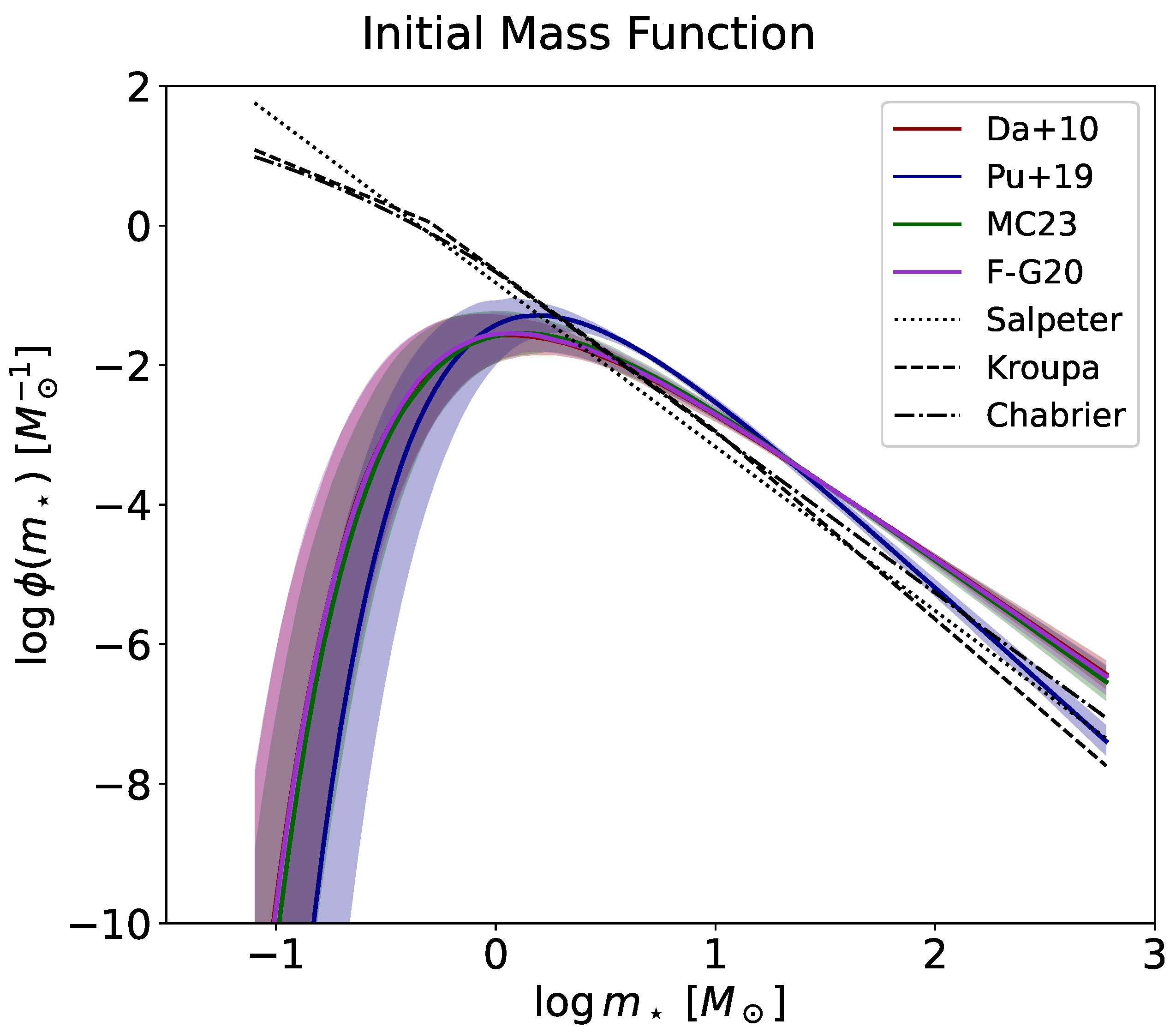
2.2. Initial Mass Function
2.3. Constraints from Galaxy Formation
2.4. Bayesian Analysis
3. Results and Discussion
4. Summary
Author Contributions
Funding
Data Availability Statement
Acknowledgments
Conflicts of Interest
References
- Kroupa, P.; Jerabkova, T. A Universal Stellar Initial Mass Function? A Critical Look at Variations. Ann. Rev. Astron. Astrophys. 2010, 48, 339. [Google Scholar]
- Krumholz, M.R. The big problems in star formation: The star formation rate, stellar clustering, and the initial mass function. Phys. Rep. 2014, 539, 49. [Google Scholar] [CrossRef]
- Kroupa, P.; Jerabkova, T. The initial mass function of stars and the star-formation rates of galaxies. In Star-Formation Rates of Galaxies; Buat, V., Zezas, A., Eds.; Cambridge University Press: Cambridge, UK, 2021. [Google Scholar] [CrossRef]
- Salpeter, E.E. The Luminosity Function and Stellar Evolution. Astrophys. J. 1955, 121, 161. [Google Scholar] [CrossRef]
- Kroupa, P. On the variation of the initial mass function. Mon. Not. R. Astron. Soc. 2001, 322, 231. [Google Scholar] [CrossRef]
- Chabrier, G. Galactic Stellar and Substellar Initial Mass Function. Publ. Astron. Soc. Pacific 2003, 115, 763. [Google Scholar] [CrossRef]
- Larson, R.B. Early star formation and the evolution of the stellar initial mass function in galaxies. Mon. Not. R. Astron. Soc. 1998, 301, 569. [Google Scholar] [CrossRef]
- Wise, J.H.; Abel, T.; Turk, M.J.; Norman, M.L.; Smith, B.D. The birth of a galaxy—II. The role of radiation pressure. Mon. Not. R. Astron. Soc. 2012, 427, 311. [Google Scholar] [CrossRef]
- Adams, F.C.; Fatuzzo, M. A Theory of the Initial Mass Function for Star Formation in Molecular Clouds. Astrophys. J. 1996, 464, 256. [Google Scholar] [CrossRef]
- Padoan, P.; Nordlund, A. The Stellar Initial Mass Function from Turbulent Fragmentation. Astrophys. J. 2002, 576, 870. [Google Scholar] [CrossRef]
- Weidner, C.; Kroupa, P. The Variation of Integrated Star Initial Mass Functions among Galaxies. Astrophys. J. 2005, 625, 754. [Google Scholar] [CrossRef]
- Hennebelle, P.; Chabrier, G. Analytical Theory for the Initial Mass Function. III. Time Dependence and Star Formation Rate. Astrophys. J. 2013, 770, 550. [Google Scholar] [CrossRef]
- Fontanot, F.; La Barbera, F.; De Lucia, G.; Pasquali, A.; Vazdekis, A. On the shape and evolution of a cosmic-ray-regulated galaxy-wide stellar initial mass function. Mon. Not. R. Astron. Soc. 2018, 479, 5678. [Google Scholar] [CrossRef]
- van Dokkum, P.G.; Conroy, C. A substantial population of low-mass stars in luminous elliptical galaxies. Nature 2010, 468, 940. [Google Scholar] [CrossRef]
- Martin-Navarro, I.; Vazdekis, A.; La Barbera, F.; Falcon-Barroso, J.; Lyubenova, M.; van de Ven, G.; Ferreras, I.; Sanchez, S.F.; Trager, S.C.; Garcia-Benito, R.; et al. IMF and Metallicity: A Tight Local Relation Revealed by the CALIFA Survey. Astrophys. J. 2015, 806, L31. [Google Scholar] [CrossRef]
- Cappellari, M. Structure and Kinematics of Early-Type Galaxies from Integral Field Spectroscopy. Ann. Rev. Astron. Astrophys. 2016, 54, 597. [Google Scholar] [CrossRef]
- Zhang, Z.-Y.; Romano, D.; Ivison, R.J.; Papadopoulos, P.P.; Matteucci, F. Stellar populations dominated by massive stars in dusty starburst galaxies across cosmic time. Nature 2018, 558, 260. [Google Scholar] [CrossRef]
- Li, J.; Liu, C.; Zhang, Z.-Y.; Tian, H.; Fu, X.; Li, J.; Yan, Z.-Q. Stellar initial mass function varies with metallicity and time. Nature 2023, 613, 460. [Google Scholar] [CrossRef]
- Aghanim, N.; Akrami, Y.; Ashdown, M.; Aumont, J.; Baccigalupi, C.; Ballardini, M.; Banday, A.J.; Barreiro, R.B.; Bartolo, N.; Basak, S.; et al. [Planck Collaboration]. Planck 2018 results. VI. Cosmological parameters. Astron. Astrophys. 2020, 641, A6. [Google Scholar]
- Becker, G.D.; Bolton, J.S. New measurements of the ionizing ultraviolet background over 2 < z<5 and implications for hydrogen reionization. Mon. Not. R. Astron. Soc. 2013, 436, 1023. [Google Scholar]
- Becker, G.D.; D’Aloisio, A.; Christenson, H.M.; Zhu, Y.; Worseck, G.; Bolton, J.S. The mean free path of ionizing photons at 5<z<6: Evidence for rapid evolution near reionization. Mon. Not. R. Astron. Soc. 2021, 508, 1853–1869. [Google Scholar]
- Konno, A.; Ouchi, M.; Ono, Y.; Shimasaku, K.; Shibuya, T.; Furusawa, H.; Nakajima, K.; Naito, Y.; Momose, R.; Yuma, S.; et al. Accelerated Evolution of the Lyα Luminosity Function at z ≳ 7 Revealed by the Subaru Ultra-deep Survey for Lyα Emitters at z=7.3. Astrophys. J. 2014, 797, 16. [Google Scholar] [CrossRef]
- McGreer, I.D.; Mesinger, A.; D’Odorico, V. Model-independent evidence in favour of an end to reionization by z≈6. Mon. Not. R. Astron. Soc. 2015, 447, 499–505. [Google Scholar] [CrossRef]
- Davies, F.B.; Hennawi, J.F.; Banados, E.; Lukic, Z.; Decarli, R.; Fan, X.; Farina, E.P.; Mazzucchelli, C.; Rix, H.-W.; Venemans, B.P.; et al. Quantitative Constraints on the Reionization History from the IGM Damping Wing Signature in Two Quasars at z > 7. Astrophys. J. 2018, 864, 142. [Google Scholar] [CrossRef]
- Mason, C.A.; Treu, T.; Dijkstra, M.; Mesinger, A.; Trenti, M.; Pentericci, L.; de Barros, S.; Vanzella, E. The Universe Is Reionizing at z∼7: Bayesian Inference of the IGM Neutral Fraction Using Lyα Emission from Galaxies. Astrophys. J. 2018, 856, 2. [Google Scholar] [CrossRef]
- Konno, A.; Ouchi, M.; Shibuya, T.; Ono, Y.; Shimasaku, K.; Taniguchi, Y.; Nagao, T.; Kobayashi, M.A.R.; Kajisawa, M.; Kashikawa, N.; et al. SILVERRUSH. IV. Lyα luminosity functions at z = 5.7 and 6.6 studied with ∼1300 Lyα emitters on the 14–21 deg2 sky. Publ. Astron. Soc. Jpn. 2018, 70, S16. [Google Scholar] [CrossRef]
- Hoag, A.; Bradac, M.; Huang, K.; Mason, C.; Treu, T.; Schmidt, K.B.; Trenti, M.; Strait, V.; Lemaux, B.C.; Finney, E.Q.; et al. Constraining the Neutral Fraction of Hydrogen in the IGM at Redshift 7.5. Astrophys. J. 2019, 878, 12. [Google Scholar] [CrossRef]
- Bolan, P.; Lemaux, B.C.; Mason, C.; Bradac, M.; Treu, T.; Strait, V.; Pelliccia, D.; Pentericci, L.; Malkan, M. Inferring the IGM Neutral Fraction at z∼ 6–8 with Low-Luminosity Lyman Break Galaxies. arXiv 2021, arXiv:2111.14912. [Google Scholar]
- Greig, B.; Mesinger, A.; Davies, F.B.; Wang, F.; Yang, J.; Hennawi, J.F. IGM damping wing constraints on reionisation from covariance reconstruction of two z ≳ 7 QSOs. Mon. Not. R. Astron. Soc. 2022, 512, 5390–5403. [Google Scholar] [CrossRef]
- Robertson, B.E.; Ellis, R.S.; Furlanetto, S.R.; Dunlop, J.S. Cosmic reionization and early star-forming galaxies: A joint analysis of new constraints from Planck and Hubble Space Telescope. Astrophys. J. 2015, 802, L19. [Google Scholar] [CrossRef]
- Finkelstein, S.L.; D’Aloisio, A.; Paardekooper, J.-P.; Ryan, R., Jr.; Behroozi, P.; Finlator, K.; Livermore, R.; Upton Sanderbeck, P.R.; Dalla Vecchia, C.; Khochfar, S. Conditions for Reionizing the Universe with a Low Galaxy Ionizing Photon Escape Fraction. Astrophys. J. 2019, 879, 36. [Google Scholar] [CrossRef]
- Lapi, A.; Ronconi, T.; Boco, L.; Shankar, F.; Krachmalnicoff, N.; Baccigalupi, C.; Danese, L. Astroparticle Constraints from Cosmic Reionization and Primordial Galaxy Formation. Universe 2022, 8, 476. [Google Scholar] [CrossRef]
- Gandolfi, G.; Lapi, A.; Ronconi, T.; Danese, L. Astroparticle Constraints from the Cosmic Star Formation Rate Density at High Redshift: Current Status and Forecasts for JWST. Universe 2022, 8, 589. [Google Scholar] [CrossRef]
- Bouwens, R.J.; Oesch, P.A.; Stefanon, M.; Illingworth, G.; Labbé, I.; Reddy, N.; Atek, H.; Montes, M.; Naidu, R.; Nanayakkara, T.; et al. New Determinations of the UV Luminosity Functions from z 9 to 2 Show a Remarkable Consistency with Halo Growth and a Constant Star Formation Efficiency. Astron. J. 2021, 162, 47. [Google Scholar] [CrossRef]
- Oesch, P.A.; Bouwens, R.J.; Illingworth, G.D.; Labbé, I.; Stefanon, M. The Dearth of z∼10 Galaxies in All HST Legacy Fields—The Rapid Evolution of the Galaxy Population in the First 500 Myr. Astrophys. J. 2018, 855, 105. [Google Scholar] [CrossRef]
- Bouwens, R.; Illingworth, G.; Oesch, P.; Stefanon, M.; Naidu, R.; van Leeuwen, I.; Magee, D. UV luminosity density results at z > 8 from the first JWST/NIRCam fields: Limitations of early data sets and the need for spectroscopy. Mon. Not. R. Astron. Soc. 2023, 523, 1009. [Google Scholar] [CrossRef]
- Bouwens, R.J.; Stefanon, M.; Brammer, G.; Oesch, P.A.; Herard-Demanche, T.; Illingworth, G.D.; Matthee, J.; Naidu, R.P.; van Dokkum, P.G.; van Leeuwen, I.F. Evolution of the UV LF from z 15 to z 8 using new JWST NIRCam medium-band observations over the HUDF/XDF. Mon. Not. R. Astron. Soc. 2023, 523, 1036. [Google Scholar] [CrossRef]
- Harikane, Y.; Ouchi, M.; Oguri, M.; Ono, Y.; Nakajima, K.; Isobe, Y.; Umeda, H.; Mawatari, K.; Zhang, Y. A Comprehensive Study of Galaxies at z 9–16 Found in the Early JWST Data: Ultraviolet Luminosity Functions and Cosmic Star Formation History at the Pre-reionization Epoch. Astrophys. J. Suppl. 2023, 265, 5. [Google Scholar] [CrossRef]
- Harikane, Y.; Nakajima, K.; Ouchi, M.; Umeda, H.; Isobe, Y.; Ono, Y.; Xu, Y.; Zhang, Y. Pure Spectroscopic Constraints on UV Luminosity Functions and Cosmic Star Formation History From 25 Galaxies at zspec = 8.61–13.20 Confirmed with JWST/NIRSpec. arXiv 2023, arXiv:2304.06658. [Google Scholar]
- Harikane, Y.; Ono, Y.; Ouchi, M.; Liu, C.; Sawicki, M.; Shibuya, T.; Behroozi, P.S.; He, W.; Shimasaku, K.; Arnouts, S.; et al. GOLDRUSH. IV. Luminosity Functions and Clustering Revealed with 4,000,000 Galaxies at z∼ 2–7: Galaxy-AGN Transition, Star Formation Efficiency, and Implication for Evolution at z > 10. Astrophys. J. Suppl. 2023, 259, 20. [Google Scholar] [CrossRef]
- Donnan, C.T.; McLeod, D.J.; Dunlop, J.S.; McLure, R.J.; Carnall, A.C.; Begley, R.; Cullen, F.; Hamadouche, M.L.; Bowler, R.A.A.; Magee, D.; et al. The evolution of the galaxy UV luminosity function at redshifts z∼ 8–15 from deep JWST and ground-based near-infrared imaging. Mon. Not. R. Astron. Soc. 2023, 518, 6011. [Google Scholar] [CrossRef]
- Donnan, C.T.; McLeod, D.J.; McLure, R.J.; Dunlop, J.S.; Carnall, A.C.; Cullen, F.; Magee, D. The abundance of z ≳ 10 galaxy candidates in the HUDF using deep JWST NIRCam medium-band imaging. Mon. Not. R. Astron. Soc. 2023, 520, 4554. [Google Scholar] [CrossRef]
- Naidu, R.P.; Oesch, P.A.; van Dokkum, P.; Nelson, E.J.; Suess, K.A.; Brammer, G.; Whitaker, K.E.; Illingworth, G.; Bouwens, R.; Tacchella, S.; et al. Two Remarkably Luminous Galaxy Candidates at z≈ 10–12 Revealed by JWST. Astrophys. J. 2022, 940, L14. [Google Scholar] [CrossRef]
- Finkelstein, S.L.; Bagley, M.B.; Ferguson, H.C.; Wilkins, S.M.; Kartaltepe, J.S.; Papovich, C.; Yung, L.Y.A.; Haro, P.A.; Behroozi, P.; Dickinson, M.; et al. CEERS Key Paper. I. An Early Look into the First 500 Myr of Galaxy Formation with JWST. Astrophys. J. 2023, 946, L13. [Google Scholar] [CrossRef]
- Dayal, P.; Volonteri, M.; Choudhury, T.R.; Schneider, R.; Trebitsch, M.; Gnedin, N.Y.; Atek, H.; Hirschmann, M.; Reines, A. Reionization with galaxies and active galactic nuclei. Mon. Not. R. Astron. Soc. 2020, 495, 3065. [Google Scholar] [CrossRef]
- Puchwein, E.; Haardt, F.; Haehnelt, M.G.; Madau, P. Consistent modelling of the meta-galactic UV background and the thermal/ionization history of the intergalactic medium. Mon. Not. R. Astron. Soc. 2019, 485, 47. [Google Scholar] [CrossRef]
- Faucher-Giguère, C.-A. A cosmic UV/X-ray background model update. Mon. Not. R. Astron. Soc. 2020, 493, 1614. [Google Scholar] [CrossRef]
- Mitra, S.; Chatterjee, A. Non-parametric reconstruction of photon escape fraction from reionization. Mon. Not. R. Astron. Soc. 2023, 523, L35. [Google Scholar] [CrossRef]
- Kulkarni, G.; Keating, L.C.; Haehnelt, M.G.; Bosman, S.E.I.; Puchwein, E.; Chardin, J.; Aubert, D. Large Lyα opacity fluctuations and low CMB τ in models of late reionization with large islands of neutral hydrogen extending to z < 5.5. Mon. Not. R. Astron. Soc. 2019, 485, L24. [Google Scholar]
- Katz, H.; Saxena, A.; Rosdahl, J.; Kimm, T.; Blaizot, J.; Garel, T.; Michel-Dansac, L.; Haehnelt, M.; Ellis, R.S.; Pentericci, L.; et al. Two modes of LyC escape from bursty star formation: Implications for [CII] deficits and the sources of reionization. Mon. Not. R. Astron. Soc. 2023, 518, 270. [Google Scholar] [CrossRef]
- Paardekooper, J.-P.; Khochfar, S.; Dalla Vecchia, C. The First Billion Years project: The escape fraction of ionizing photons in the epoch of reionization. Mon. Not. R. Astron. Soc. 2015, 451, 2544. [Google Scholar] [CrossRef]
- Vanzella, E.; Nonino, M.; Cupani, G.; Castellano, M.; Sani, E.; Mignoli, M.; Calura, F.; Meneghetti, M.; Gilli, R.; Comastri, A.; et al. Direct Lyman continuum and Lyα escape observed at redshift 4. Mon. Not. R. Astron. Soc. 2018, 476, L15. [Google Scholar] [CrossRef]
- Alavi, A.; Colbert, J.; Teplitz, H.I.; Siana, B.; Scarlata, C.; Rutkowski, M.; Mehta, V.; Henry, A.; Dai, Y.S.; Haardt, F.; et al. Lyman Continuum Escape Fraction from Low-mass Starbursts at z = 1.3. Astrophys. J. 2020, 904, 59. [Google Scholar] [CrossRef]
- Smith, B.M.; Windhorst, R.A.; Cohen, S.H.; Koekemoer, A.M.; Jansen, R.A.; White, C.; Borthakur, S.; Hathi, N.; Jiang, L.; Rutkowski, M.; et al. The Lyman Continuum Escape Fraction of Galaxies and AGN in the GOODS Fields. Astrophys. J. 2020, 897, 41. [Google Scholar] [CrossRef]
- Izotov, Y.I.; Worseck, G.; Schaerer, D.; Guseva, N.G.; Chisholm, J.; Thuan, T.X.; Fricke, K.J.; Verhamme, A. Lyman continuum leakage from low-mass galaxies with M⋆<108 M⊙. Mon. Not. R. Astron. Soc. 2021, 503, 1734. [Google Scholar]
- Pahl, A.J.; Shapley, A.; Steidel, C.C.; Chen, Y.; Reddy, N.A. An uncontaminated measurement of the escaping Lyman continuum at z∼3. Mon. Not. R. Astron. Soc. 2021, 505, 2447. [Google Scholar] [CrossRef]
- Atek, H.; Furtak, L.J.; Oesch, P.; van Dokkum, P.; Reddy, N.; Contini, T.; Illingworth, G.; Wilkins, S. The star formation burstiness and ionizing efficiency of low-mass galaxies. Mon. Not. R. Astron. Soc. 2022, 511, 4464. [Google Scholar] [CrossRef]
- Naidu, R.P.; Matthee, J.; Oesch, P.A.; Conroy, C.; Sobral, D.; Pezzulli, G.; Hayes, M.; Erb, D.; Amorín, R.; Gronke, M.; et al. The synchrony of production and escape: Half the bright Lyα emitters at z ≈ 2 have Lyman continuum escape fractions ≈50%. Mon. Not. R. Astron. Soc. 2022, 510, 4582. [Google Scholar] [CrossRef]
- Khaire, V.; Srianand, R. New synthesis models of consistent extragalactic background light over cosmic time. Mon. Not. R. Astron. Soc. 2019, 484, 4174. [Google Scholar] [CrossRef]
- Cain, C.; D’Aloisio, A.; Gangolli, N.; Becker, G.D. A Short Mean Free Path at z = 6 Favors Late and Rapid Reionization by Faint Galaxies. Astrophys. J. 2021, 917, L37. [Google Scholar] [CrossRef]
- Steidel, C.C.; Bogosavljevic, M.; Shapley, A.E.; Reddy, N.A.; Rudie, G.C.; Pettini, M.; Trainor, R.F.; Strom, A.L. The Keck Lyman Continuum Spectroscopic Survey (KLCS): The Emergent Ionizing Spectrum of Galaxies at z∼3. Astrophys. J. 2018, 869, 123. [Google Scholar] [CrossRef]
- Fletcher, T.J.; Tang, M.; Robertson, B.E.; Nakajima, K.; Ellis, R.S.; Stark, D.P.; Inoue, A. The Lyman Continuum Escape Survey: Ionizing Radiation from [OIII]-strong Sources at a Redshift of 3.1. Astrophys. J. 2019, 878, 87. [Google Scholar] [CrossRef]
- Kennicutt, R.C.; Evans, N.J. Star Formation in the Milky Way and Nearby Galaxies. Annu. Rev. Astron. Astrophys. 2012, 50, 531–608. [Google Scholar] [CrossRef]
- Madau, P.; Dickinson, M. Cosmic Star-Formation History. Annu. Rev. Astron. Astrophys. 2014, 52, 415. [Google Scholar] [CrossRef]
- Cai, Z.; Lapi, A.; Bressan, A.; De Zotti, G.; Negrello, M.; Danese, L. A Physical Model for the Evolving Ultraviolet Luminosity Function of High Redshift Galaxies and their Contribution to the Cosmic Reionization. Astrophys. J. 2014, 785, 65. [Google Scholar] [CrossRef]
- Bose, S.; Deason, A.J.; Frenk, C.S. The Imprint of Cosmic Reionization on the Luminosity Function of Galaxies. Astrophys. J. 2018, 863, 123. [Google Scholar] [CrossRef]
- Romanello, M.; Menci, N.; Castellano, M. The Epoch of Reionization in Warm Dark Matter Scenarios. Universe 2021, 7, 365. [Google Scholar] [CrossRef]
- Munoz, J.B.; Qin, Y.; Mesinger, A.; Murray, S.G.; Greig, B.; Mason, C. The impact of the first galaxies on cosmic dawn and reionization. Mon. Not. R. Astron. Soc. 2022, 511, 3657–3681. [Google Scholar] [CrossRef]
- Bouwens, R.J.; Illingworth, G.; Ellis, R.S.; Oesch, P.A.; Stefanon, M. z∼2-9 galaxies magnified by the Hubble Frontier Field Clusters II: Luminosity functions and constraints on a faint end turnover. Astrophys. J. 2022, 940, 55. [Google Scholar] [CrossRef]
- Mao, J.; Lapi, A.; Granato, G.L.; de Zotti, G.; Danese, L. The Role of the Dust in Primeval Galaxies: A Simple Physical Model for Lyman Break Galaxies and Ly-α Emitters. Astrophys. J. 2007, 667, 655. [Google Scholar] [CrossRef][Green Version]
- Rutkowski, M.J.; Scarlata, C.; Haardt, F.; Siana, B.; Henry, A.; Rafelski, M.; Hayes, M.; Salvato, M.; Pahl, A.J.; Mehta, V.; et al. Lyman Continuum Escape Fraction of Star-forming Dwarf Galaxies at z∼1. Astrophys. J. 2016, 819, 81. [Google Scholar] [CrossRef]
- Shen, X.; Hopkins, P.F.; Faucher-Giguère, C.-A.; Alexander, D.M.; Richards, G.T.; Ross, N.P.; Hickox, R.C. The bolometric quasar luminosity function at z = 0–7. Mon. Not. R. Astron. Soc. 2020, 495, 3252–3275. [Google Scholar] [CrossRef]
- Shankar, F.; Mathur, S. On the Faint End of the High-Redshift Active Galactic Nucleus Luminosity Function. Astrophys. J. 2007, 660, 1051. [Google Scholar] [CrossRef]
- Giallongo, E.; Grazian, A.; Fiore, F.; Fontana, A.; Pentericci, L.; Vanzella, E.; Dickinson, M.; Kocevski, D.; Castellano, M.; Cristiani, S.; et al. Faint AGNs at z > 4 in the CANDELS GOODS-S field: Looking for contributors to the reionization of the Universe. Astron. Astrophys. 2015, 578, A83. [Google Scholar] [CrossRef]
- Ricci, F.; Marchesi, S.; Shankar, F.; La Franca, F.; Civano, F. Constraining the UV emissivity of AGN throughout cosmic time via X-ray surveys. Mon. Not. R. Astron. Soc. 2017, 465, 1915–1925. [Google Scholar] [CrossRef]
- Giallongo, E.; Grazian, A.; Fiore, F.; Kodra, D.; Urrutia, T.; Castellano, M.; Cristiani, S.; Dickinson, M.; Fontana, A.; Menci, N.; et al. Space Densities and Emissivities of Active Galactic Nuclei at z > 4. Astrophys. J. 2019, 884, 19. [Google Scholar] [CrossRef]
- Kulkarni, G.; Worseck, G.; Hennawi, J.F. Evolution of the AGN UV luminosity function from redshift 7.5. Mon. Not. R. Astron. Soc. 2019, 488, 1035–1065. [Google Scholar] [CrossRef]
- Ananna, T.T.; Urry, C.M.; Treister, E.; Hickox, R.C.; Shankar, F.; Ricci, C.; Cappelluti, N.; Marchesi, S.; Turner, T.J. Accretion History of AGNs. III. Radiative Efficiency and AGN Contribution to Reionization. Astrophys. J. 2020, 903, 85. [Google Scholar] [CrossRef]
- Grazian, A.; Giallongo, E.; Boutsia, K.; Cristiani, S.; Vanzella, E.; Scarlata, C.; Santini, P.; Pentericci, L.; Merlin, E.; Menci, N.; et al. The contribution of faint AGNs to the ionizing background at z > 4. Astron. Astrophys. 2018, 613, A44. [Google Scholar] [CrossRef]
- Romano, M. Lyman continuum escape fraction and mean free path of hydrogen ionizing photons for bright z∼4 QSOs from SDSS DR14. Astron. Astrophys. 2019, 632, A45. [Google Scholar] [CrossRef]
- Madau, P.; Haardt, F.; Rees, M.J. Radiative transfer in a clumpy Universe. III. The nature of cosmological ionizing sources. Astrophys. J. 1999, 514, 648. [Google Scholar] [CrossRef]
- Loeb, A.; Barkana, R. The Reionization of the Universe by the First Stars and Quasars. Annu. Rev. Astron. Astrophys. 2001, 39, 19–66. [Google Scholar] [CrossRef]
- Pawlik, A.H.; Schaye, J.; van Scherpenzeel, E. Keeping the Universe ionized: Photoheating and the clumping factor of the high-redshift intergalactic medium. Mon. Not. R. Astron. Soc. 2009, 394, 1812–1824. [Google Scholar] [CrossRef]
- Haardt, F.; Madau, P. Radiative Transfer in a Clumpy Universe. IV. New Synthesis Models of the Cosmic UV/X-Ray Background. Astrophys. J. 2012, 746, 125. [Google Scholar] [CrossRef]
- Schneider, F.R.N.; Ramírez-Agudelo, O.H.; Tramper, F.; Bestenlehner, J.M.; Castro, N.; Sana, H.; Evans, C.J.; Sabín-Sanjulián, C.; Simón-Díaz, S.; Langer, N.; et al. The VLT-FLAMES Tarantula Survey. XXIX. Massive star formation in the local 30 Doradus starburst. Astron. Astrophys. 2018, 618, A73. [Google Scholar] [CrossRef]
- Goswami, S.; Silva, L.; Bressan, A.; Grisoni, V.; Costa, G.; Marigo, P.; Granato, G.L.; Lapi, A.; Spera, M. Impact of very massive stars on the chemical evolution of extremely metal-poor galaxies. Astron. Astrophys. 2022, 663, A1. [Google Scholar] [CrossRef]
- Bressan, A.; Marigo, P.; Girardi, L.; Salasnich, B.; Dal Cero, C.; Rubele, S.; Nanni, A. PARSEC: Stellar tracks and isochrones with the PAdova and TRieste Stellar Evolution Code. Mon. Not. R. Astron. Soc. 2012, 427, 127. [Google Scholar] [CrossRef]
- Efstathiou, G. Suppressing the formation of dwarf galaxies via photoionization. Mon. Not. R. Astron. Soc. 1992, 256, 43. [Google Scholar] [CrossRef]
- Sobacchi, E.; Mesinger, A. How does radiative feedback from an ultraviolet background impact reionization? Mon. Not. R. Astron. Soc. 2013, 432, 3340. [Google Scholar] [CrossRef]
- Aversa, R.; Lapi, A.; De Zotti, G.; Danese, L. Black Hole and Galaxy Coevolution from Continuity Equation and Abundance Matching. Astrophys. J. 2015, 810, 74. [Google Scholar] [CrossRef]
- Moster, B.P.; Naab, T.; White, S.D.M. EMERGE—An empirical model for the formation of galaxies since z∼10. Mon. Not. R. Astron. Soc. 2018, 477, 1822. [Google Scholar] [CrossRef]
- Cristofari, P.; Ostriker, J.P. Abundance matching for low-mass galaxies in the CDM and FDM models. Mon. Not. R. Astron. Soc. 2019, 482, 4364. [Google Scholar] [CrossRef]
- Behroozi, P.; Wechsler, R.H.; Hearin, A.P.; Conroy, C. UNIVERSEMACHINE: The correlation between galaxy growth and dark matter halo assembly from z = 0–10. Mon. Not. R. Astron. Soc. 2020, 488, 3143. [Google Scholar] [CrossRef]
- Tinker, J.; Kravtsov, A.V.; Klypin, A.; Abazajian, K.; Warren, M.; Yepes, G.; Gottlober, S.; Holz, D.E. Toward a Halo Mass Function for Precision Cosmology: The Limits of Universality. Astrophys. J. 2008, 688, 709. [Google Scholar] [CrossRef]
- Diemer, B. COLOSSUS: A Python Toolkit for Cosmology, Large-scale Structure, and Dark Matter Halos. Astrophys. J. Suppl. Ser. 2018, 239, 35. [Google Scholar] [CrossRef]
- Moster, B.P.; Naab, T.; White, S.D.M. Galactic star formation and accretion histories from matching galaxies to dark matter haloes. Mon. Not. R. Astron. Soc. 2013, 428, 3121. [Google Scholar] [CrossRef]
- Lange, J.U.; van den Bosch, F.C.; Zentner, A.R.; Wang, K.; Villarreal, A.S. Updated results on the galaxy-halo connection from satellite kinematics in SDSS. Mon. Not. R. Astron. Soc. 2019, 487, 3112. [Google Scholar] [CrossRef]
- Lapi, A.; Salucci, P.; Danese, L. Precision Scaling Relations for Disk Galaxies in the Local Universe. Astrophys. J. 2018, 859, 2. [Google Scholar] [CrossRef]
- Mandelbaum, R.; Wang, W.; Zu, Y.; White, S.; Henriques, B.; More, S. Strong bimodality in the host halo mass of central galaxies from galaxy-galaxy lensing. Mon. Not. R. Astron. Soc. 2016, 457, 3002. [Google Scholar] [CrossRef]
- Foreman-Mackey, D.; Hogg, D.W.; Lang, D.; Goodman, J. emcee: The MCMC Hammer. Publ. Astron. Soc. Pac. 2013, 125, 306. [Google Scholar] [CrossRef]
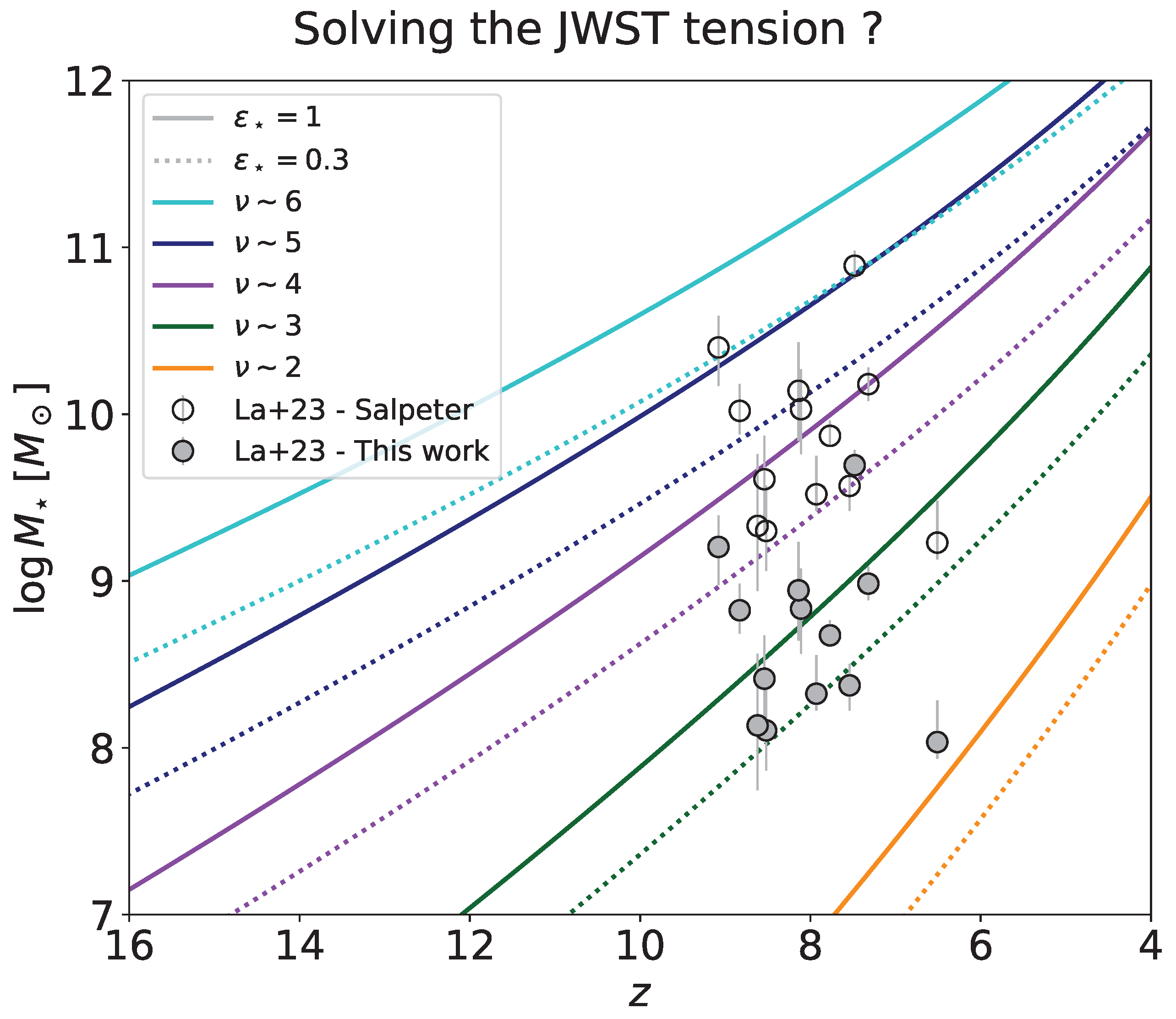
- Labbe, I.; van Dokkum, P.; Nelson, E.; Bezanson, R.; Suess, K.A.; Leja, J.; Brammer, G.; Whitaker, K.; Mathews, E.; Stefanon, M.; et al. A population of red candidate massive galaxies 600 Myr after the Big Bang. Nature 2023, 616, 266. [Google Scholar] [CrossRef]
- Curtis-Lake, E.; Carniani, S.; Cameron, A.; Charlot, S.; Jakobsen, P.; Maiolino, R.; Bunker, A.; Witstok, J.; Smit, R.; Chevallard, J.; et al. Spectroscopic confirmation of four metal-poor galaxies at z = 10.3–13.2. Nature Astron. 2023, 7, 622. [Google Scholar] [CrossRef]
- Boylan-Kolchin, M. Stress testing ΛCDM with high-redshift galaxy candidates. Nature Astron. 2023, 7, 731. [Google Scholar] [CrossRef]


| Observable [Units] | Redshifts | Values | Uncertainty | Ref. |
|---|---|---|---|---|
| [ s−1 Mpc−3] | ||||
| [20] | ||||
| [21] | ||||
| [25] | ||||
| [27] | ||||
| [22,26] | ||||
| [28] | ||||
| [29] | ||||
| [24] | ||||
| [23] | ||||
| [19] |
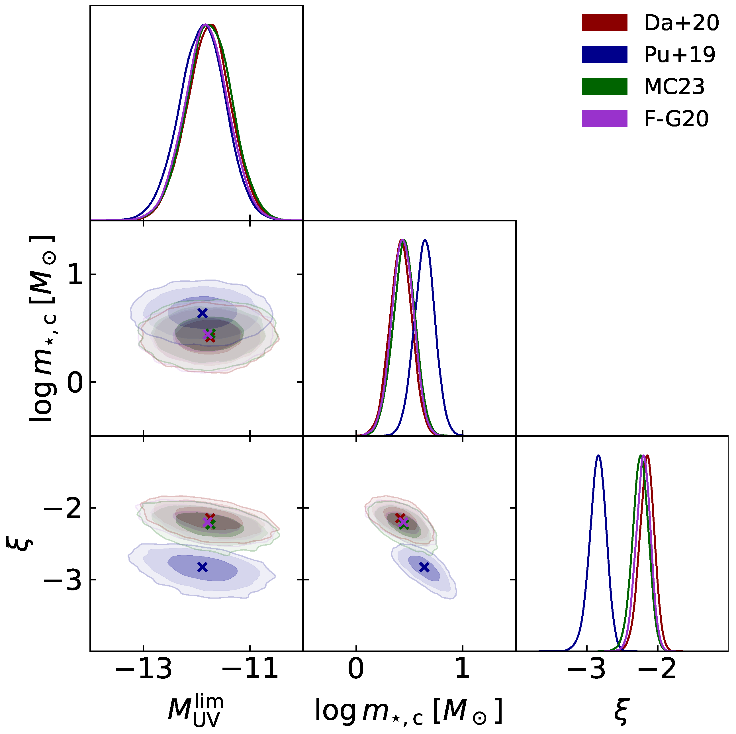
| Da+20 [45] | [−11.75] | [0.42] | [−2.15] | |
| Pu+19 [46] | [−11.89] | [0.64] | [−2.83] | |
| F-G20 [47] | [−11.79] | [0.44] | [−2.20] | |
| MC23 [48] | [−11.74] | [0.45] | [−2.23] |
Disclaimer/Publisher’s Note: The statements, opinions and data contained in all publications are solely those of the individual author(s) and contributor(s) and not of MDPI and/or the editor(s). MDPI and/or the editor(s) disclaim responsibility for any injury to people or property resulting from any ideas, methods, instructions or products referred to in the content. |
© 2024 by the authors. Licensee MDPI, Basel, Switzerland. This article is an open access article distributed under the terms and conditions of the Creative Commons Attribution (CC BY) license (https://creativecommons.org/licenses/by/4.0/).
Share and Cite
Lapi, A.; Gandolfi, G.; Boco, L.; Gabrielli, F.; Massardi, M.; Haridasu, B.S.; Baccigalupi, C.; Bressan, A.; Danese, L. Constraining the Initial Mass Function in the Epoch of Reionization from Astrophysical and Cosmological Data. Universe 2024, 10, 141. https://doi.org/10.3390/universe10030141
Lapi A, Gandolfi G, Boco L, Gabrielli F, Massardi M, Haridasu BS, Baccigalupi C, Bressan A, Danese L. Constraining the Initial Mass Function in the Epoch of Reionization from Astrophysical and Cosmological Data. Universe. 2024; 10(3):141. https://doi.org/10.3390/universe10030141
Chicago/Turabian StyleLapi, Andrea, Giovanni Gandolfi, Lumen Boco, Francesco Gabrielli, Marcella Massardi, Balakrishna S. Haridasu, Carlo Baccigalupi, Alessandro Bressan, and Luigi Danese. 2024. "Constraining the Initial Mass Function in the Epoch of Reionization from Astrophysical and Cosmological Data" Universe 10, no. 3: 141. https://doi.org/10.3390/universe10030141
APA StyleLapi, A., Gandolfi, G., Boco, L., Gabrielli, F., Massardi, M., Haridasu, B. S., Baccigalupi, C., Bressan, A., & Danese, L. (2024). Constraining the Initial Mass Function in the Epoch of Reionization from Astrophysical and Cosmological Data. Universe, 10(3), 141. https://doi.org/10.3390/universe10030141