Abstract
Swarm intelligence (SI) methods are nature-inspired metaheuristics for global optimization that exploit a coordinated stochastic search strategy by a group of agents. Particle swarm optimization (PSO) is an established SI method that has been applied successfully to the optimization of rugged high-dimensional likelihood functions, a problem that represents the main bottleneck across a variety of gravitational wave (GW) data analysis challenges. We present results from the first application of PSO to one of the most difficult of these challenges, namely the search for the Extreme Mass Ratio Inspiral (EMRI) in data from future spaceborne GW detectors such as LISA, Taiji, or Tianqin. We use the standard Generalized Likelihood Ratio Test formalism, with the minimal use of restrictive approximations, to search 6 months of simulated LISA data and quantify the search depth, signal-to-noise ratio (SNR), and breadth, within the ranges of the EMRI parameters, that PSO can handle. Our results demonstrate that a PSO-based EMRI search is successful for a search region ranging over ≳10σ for the majority of parameters and ≳200σ for one, with being the SNR-dependent Cramer–Rao lower bound on the parameter estimation error and . This is in the vicinity of the search ranges that the current hierarchical schemes can identify. Directions for future improvement, including computational bottlenecks to be overcome, are identified.
1. Introduction
Spaceborne gravitational wave (GW) detectors, namely LISA [1] and the planned Taiji [2,3] and Tianqin [4], are expected to observe long-lived signals from a variety of sources in the mHz regime. Among these would be the large population of compact object binaries [5,6,7] in the Milky Way, the binaries of massive black holes [8,9,10], and Extreme Mass Ratio Inspirals (EMRI) [11,12,13,14,15], consisting of a massive black hole orbited by a much smaller one. Extracting individual GW signals from this crowded superposition poses a huge data analysis challenge that has mostly been addressed only for specific types of sources. For example, much work has been done to address the extraction of individual signals from the Galactic Binary population, where both the global fit [16,17] and iterative subtraction approaches [18,19,20,21] have been developed to a mature level. On the other hand, progress in the detection and estimation of even single EMRI signals has been much more modest given the extreme challenges that it involves: it is estimated that a deterministic matched filter-based search for a single EMRI signal would require ∼1040 distinct template waveforms [11]. Given that the correlation of ∼2 years of data with an equally long template involves ∼ floating point operations, the computational cost of the straightforward approach is insurmountable, even with projected advances in computing hardware.
The sheer complexity of the data analysis challenge confronting space-based GW detection necessitates the exploration and development of diverse methods. To provide a common baseline for the comparison of these methods, a series of public data analysis challenges have been provided by the community. Among these, the Mock LISA Data Challenges (MLDCs) [22,23], now called the LISA Data Challenges (LDCs) [24], and the recent Taiji Data Challenge [25] have fostered the development of a number of new data analysis methods. These include a number of different lines of attack for the EMRI problem that may be roughly divided into parametric and nonparametric approaches, with some overlap between the two. Parametric methods use parametrized waveform models, either physical or empirical, while nonparametric methods [26] avoid their use. It is important to note here that the calculation of the exact EMRI waveform is itself an open problem that is being actively addressed by several groups. Hence, all parametric approaches use surrogate models that are assumed to be sufficiently realistic while being computationally cheap to calculate. Among the main surrogate waveforms used in the literature, and also the one used in the mock data challenges, is the Analytical Kludge (AK) developed in [27], which is based on the quadrupolar waveform for an eccentric orbit [28,29] with post-Newtonian corrections to the procession of the pericenter and orbital plane, as well as the GW radiation reaction-driven inspirals. The AK waveform can be expressed as a sum over sinusoidal signals with harmonically separated frequencies that change over time following orbital evolution.
The end goal for all parametric methods is to find the global maximum of a fitness function defined over the high-dimensional space of EMRI signal parameters, with the fitness function in most cases being the log-likelihood ratio (LLR) [30] or the closely related Bayesian posterior probability [31]. The LLR at a given point in the signal parameter space for the case of Gaussian noise is simply the projection (modulo terms that take care of signal normalization) of the given data on the signal waveform, called the template, corresponding to that point. As mentioned earlier, the global maximization task is computationally infeasible if addressed using a brute force deterministic strategy, which leaves a stochastic global optimization method or a hierarchical search strategy (or their combination) as the only viable way forward. The trade-off here is between the computational feasibility and the lack of certainty in locating the global optimum, since stochastic or hierarchical methods are not provably convergent in a time-limited search (but may be asymptotically convergent).
The most popular class of stochastic global optimization methods for the EMRI problem so far has been those based on modifications of the Markov Chain Monte Carlo (MCMC) sampler [32,33,34,35,36,37,38]. Hierarchical searches [32,33,35,36,37,38] use several levels of progressively higher-fidelity approximations to the fitness function to find, with a manageable computational cost, promising search regions in the parameter space that can be handed off to a computationally expensive stochastic or deterministic global optimizer. The fitness approximations are often implemented through waveform restrictions, such as limiting the number of harmonics or duration. Most methods proposed so far need to combine elements of both the stochastic and hierarchical approaches to work well. Due to the various possibilities in how the fitness function approximations can be implemented, as well as the large number of tunable parameters that they create, the methods proposed so far tend to be quite complex in nature and involve many ad hoc design choices.
In addition to reducing the computational cost of the fitness evaluation, one of the objectives of the approximations is to mitigate the problem of secondary maxima in the exact fitness function [32,36,39] arising from complex degeneracies between the EMRI parameters and the overlap of multiple harmonics. These secondary maxima are numerous and widely dispersed in the parameter space, with values that are comparable to the global maximum. While their presence makes the problem of detection fairly easy, since locating any strong peak is an indication that the data are not pure noise, they have the adverse effect of creating large errors in the estimated signal parameters. In a multiple signal resolution problem, such as the one that all space-based detectors will face, the parameter estimation problem is equally important to that of detection, because individual sources must be fitted out from the data in order to reveal weaker sources.
It is commonly assumed, although by no means proven, that a hierarchical search should narrow down the search range to ≈100 in each signal parameter [36], where is the Cramer–Rao lower bound (CRLB) on the estimation error [30] obtained from the Fisher information matrix (FIM) at a certain signal-to-noise ratio (SNR). While serving well as a rule of thumb, we note that the search ranges suggested in the Mock LISA Data Challenge (MLDC) [22,23,40] do not obey this rule (when scaled to the same data duration) and deviate significantly from in all directions, ranging from ∼ to ∼ for some of the signal parameters at an over year data.
In this paper, we present a novel approach to the challenge of EMRI data analysis using the particle swarm optimization (PSO) [41,42,43] algorithm for the global optimization of the LLR. While PSO is a well-known stochastic optimization method that has been highly successful in a wide variety of GW data analysis problems [44,45,46,47,48,49,50,51,52,53], as well as related problems in high-dimensional statistical regression [54,55,56], it has not been applied to the EMRI problem yet (the application of PSO to the EMRI problem has been proposed in [35] but not actually implemented). The key feature of PSO that sets it apart from MCMC-based searches and makes its application to the EMRI problem attractive is its small set of tunable parameters (only two in most cases) and the significantly smaller number of LLR evaluations that it typically needs for successful convergence to the global optimum. For example, in the search for binary inspiral signals using a network of ground-based detectors, PSO has been demonstrated to need ≈10 times fewer LLR evaluations [45,46,47] than MCMC searches.
Our main objective in this paper is to conduct an ab initio investigation that removes as many ad hoc choices from the search method as possible and to focus on the end stage of any hierarchical search in which the global optimization is over the approximation-free LLR. In particular, we wish to empirically establish the baseline that a hierarchical search should target when narrowing down the search space range. We lift as many restrictions on the fitness function as computationally feasible, such as using a template waveform that includes the 10 loudest harmonics instead of 3 [32]. Similarly, we do not use approximations that attempt to subdivide the set of signal parameters into analytically maximized extrinsic and numerically maximized intrinsic, since, strictly speaking, such a division does not exist for the EMRI waveform, except for the overall distance to the source. Instead, we numerically maximize over all the parameters (except the distance), albeit using different maximization algorithms for the different subsets. Thus, our study provides a good foundation on which to build a PSO-based hierarchical search method in the future, which could provide another competitive and promising approach to address the EMRI data analysis challenge.
Within the present computational resource constraints on our analysis, we find that the PSO-based search can successfully handle the global optimization problem for EMRI signals in ≳ years of data over search ranges of ≳ for the majority of parameters and up to ≳ for one parameter. This is demonstrated over progressively weaker signal-to-noise ratios (SNRs) ranging from 50 to 30, with dependent on the SNR. We also report on the parameter estimation accuracy achieved in each case. We note that all our results establish lower bounds on the search ranges, since our code is not yet fully optimized to take advantage of graphics processing units (GPUs), and we have not been able to extend the number of PSO iterations or runs to the levels that may be needed at the lowest SNR. Nonetheless, our results show that the basic PSO is already able to handle search ranges that are in the vicinity of rule-of-thumb values, without requiring overly restrictive approximations.
The rest of the paper is organized as follows. Section 2 sets the foundation for the EMRI data analysis problem, with a review of the TDI combinations, noise, and signal models used in this paper. Section 3 describes the search method, along with the implementation and computational details. We provide a brief review of the PSO algorithm in Section 4 that is not comprehensive but suffices for the purposes of this paper. We present our results in Section 5, followed by a discussion in Section 6.
2. Data Description
The design of all space-based GW detectors consists of a constellation of spacecraft on near-Keplerian orbits, with the continuous measurement of the inter-spacecraft distances through the exchange of laser light signals. The technique of time-delay interferometry (TDI) [57] is used to reduce the dominant noise source, namely laser frequency noise, to a level where the distance fluctuations caused by incident GW signals become detectable. In TDI, the measured time-dependent inter-spacecraft distances along each arm and direction of laser light propagation are combined after being shifted by known time delays relative to each other. The combinations of delays and single-arm measurements must take a number of physical effects into account, with an increasing number of effects incorporated in successively better generations of TDI. We discuss below the TDI combinations used in this paper, followed by the description of the noise and signal models. Throughout the paper, we follow the coordinate conventions defined in [58].
2.1. TDI Combinations
In this paper, we use first-generation TDI and the combinations called A, E, and T that have mutually independent noise. They are constructed out of the Michelson TDI combinations X, Y, and Z using
where the combinations X, Y, and Z are obtained from the single-arm length measurements, , following
with s and r labeling the sender and receiver spacecraft, respectively, and l labeling the direction of laser light propagation. The expression for the single-arm response to GW, , is given by
where the vectors , , denote the position of the i-th spacecraft, the unit vector along the l-th arm, and the direction of GW propagation, respectively. The length, , of the i-th arm is approximated as constant in the first-generation TDI. The quantity , given by
is the strain response of arm l in the long-wavelength approximation, with being antenna pattern function and being the two GW polarization waveforms of a plane wave in the transverse-traceless gauge. The antenna patterns are defined by
with being the polarization angle and the defined by
where are the polarization tensors in the fiducial wave frame (as defined in [58]), which depend on the sky location of the GW source. Here, the symbol denotes the contraction operation on arbitrary tensors U and V, and, for arbitrary vectors a and b, . Of the three TDI combinations, A, E, and T, the first two carry a significantly larger GW strain response from a given source than the latter. Therefore, the combination T is generally omitted fro GW search considerations. When generating the TDI combinations for a given source, we compute the 24 time-delayed single-arm responses, , before linearly combining them, following Equation (2), to obtain X, Y, Z.
In data analysis, one works with a finite-length, uniformly sampled time series represented as a row matrix , where and , with being the sampling interval. Typically, mock LISA data are generated with s, which corresponds to a maximum frequency bandwidth of mHz, following the Nyquist sampling theorem. In searches for specific types of signals, computational savings may be obtained by resampling the data to have a higher if the maximum frequency bandwidth of the signals involved is lower. However, directly undersampling a TDI combination by computing the samples of the single-arm responses, , with a larger , causes significant numerical error when introducing the time shifts required in Equation (3) since they are smaller than even the sampling interval of 15 s. Therefore, in this paper, we keep the original LDC sampling interval when generating the GW strain responses and the TDI combinations, although the implementation of downsampling is clearly an easy choice to speed up our codes in the future.
Each TDI combination can be described by the data model,
where denotes the TDI combination I, with ; denotes the GW strain signal; and denotes the noise realization. Note that in the case of multiple overlapping GW signals, can be split into a sum of resolvable signals and unresolved signals. The latter contribute to the noise realization along with sources of instrumental noise. In this paper, in line with most other studies of the EMRI problem, we consider the simplified problem where is purely instrumental noise and is the signal from a single GW source.
2.2. Noise Model and Signal-to-Noise Ratio
Due to the lack of real data, the noise realization in most studies of LISA data analysis is assumed to be from a stationary Gaussian noise process. The LDC manual [58] provides theoretically derived analytical expressions for the power spectral densities (PSDs) of the noise processes in the TDI combinations. For the PSDs of the A and E combinations, the expressions are
where f is the Fourier frequency, is the corresponding angular frequency, and L is the (assumed constant) arm length. Under the specific noise model called SciRDv1, the acceleration noise and the Instrumental/Optical Metrology System noise are given by [59]
Given the PSD and the assumption of Gaussianity, a natural inner product can be defined on the vector space of equal-length finite time series as
where denotes the DFT of a time series ,
and , , with T being the data duration in seconds. We note that, logically, the inner product notation above should also carry the TDI index due to the dependence on the respective PSD. However, we only deal with the combinations A and E in this paper, and the two have identical PSDs. Therefore, for simplicity of notation, we have dropped the index on the inner product symbol. In terms of the inner product, one can define the SNR of a signal as
It should be noted that, due to the presence of noise, the SNR of an estimated signal will differ by a random amount from that of the true signal in the data. It is also useful to define the overlap between two signals, , as
The overlap plays a key role [22] in the context of resolving multiple sources to determine if an estimated signal matches any of a set of true signals. In the case of a single EMRI signal, the overlap between the estimated and true signals (in simulated data) can serve to indicate the presence of degeneracies in the parameter space that show up as a large overlap despite large parameter estimation errors. In addition to using both TDI combinations for overlap, one can also define the overlap between individual combinations by setting the other combination to zero. These will be designated as and , corresponding to setting and , respectively, in Equation (15).
2.3. Signal Model: EMRI Waveform
As mentioned earlier, the current standard EMRI waveform used in studies of data analysis methods as well as the LDCs is the AK waveform. In total, the AK waveform is characterized by 14 parameters: {, M, , , , , , , , , , , , D}. Here, and M represent the masses of the compact objects (COs) and the massive black hole (MBH), respectively. The parameter corresponds to the inclination angle between the angular momentum of the COs and the spin direction of MBH. denotes the magnitude of the MBH’s spin. The parameters , , , , and refer to the initial eccentricity, the initial orbital frequency, and the initial angles associated with the orbit rotation, the pericenter procession, and the Lense–Thirring precession, respectively. The angles and represent the ecliptic colatitude and longitude, respectively, of the sky location of the source in the SSB frame and , represent the polar and azimuthal angles, respectively, of the MBH spin in the SSB frame. Finally, D represents the distance between the source and the SSB center. The polarization angle depends on , , , and and stays constant in a static source frame [32].
To obtain the AK waveform for a given set of signal parameters, the ordinary differential equations (ODEs) given below need to be solved for the mean anomaly , the orbital frequency , the azimuthal angle of the pericenter precession , the eccentricity of the orbit e, and the azimuthal angle of the Lense–Thirring precession .
Since the ODEs generally evolve slowly, we follow the solution described in [58] of using a fifth-order Cash–Karp Runge–Kutta ODE solver [60] with a cadence of 15,360 s, corresponding to a timescale of a few hours, followed by interpolating the solution to a cadence of 15 seconds. Having acquired the solutions to the ODEs, one proceeds to compute the GW polarization waveforms as described schematically below.
Denoting the combined initial phase of the i-th harmonic as , , (the map from n and m to i being unimportant here) and absorbing amplitude factors such as that are common to all harmonics in an overall parameter A, we obtain
where is the set of 14 EMRI parameters, denotes the 13 parameters other than A, and denotes the 10 parameters excluding A, , , and . Thus, and . In agreement with the number of parameters that they depend on, we call , , and the 14, 13, and 10-dimensional polarization waveforms, respectively. (The expression for is provided in [58].) As with the calculation of single-arm responses, the calculation of the harmonics is parallelized in our code (using OpenMP [61]) before they are summed, which speeds up the calculation of the polarization waveforms substantially.
3. Generalized Likelihood Ratio Test
3.1. LLR
Under the assumption of Gaussian stationary noise, the log-likelihood (LLR) of the data, , , described in Section 2, is given by
To distinguish the true but unknown signal present in the data from , which is used in the evaluation of the LLR at a given point in the parameter space, the latter is called a template.
In both the Generalized Likelihood Ratio Test (GLRT) and Maximum Likelihood Estimation (MLE), the LLR is maximized over ,
with the value, , of the global maximum serving as the detection statistic, and its location, , providing the estimated values of the parameters. The parameter A can always be maximized over analytically by solving for , which gives
with the maximizer being
In the following, we call the 13-dimensional log-likelihood, with further layers of maximization producing functions that will be referred to by the corresponding number of parameters that are not maximized over. The search for the global maximum of over the 13 parameters, , in Equation (25) is the main challenge in EMRI data analysis, since the number of evaluation points required in a grid-based search is incredibly large.
A dimensionality reduction method was proposed in [32] that attempts to split the maximization of into a nested analytical inner maximization over the three initial angles, , , , and an outer numerical maximization over the remaining parameters . Briefly, this method is based on the fact that by combining the antenna patterns of a given arm l with the 13-dimensional polarization waveform (c.f., Equation (21)), the corresponding 13-dimensional single-arm strain response arising from the i-th harmonic is expressed as
Due to linearity, it follows that the TDI signal generated by the i-th harmonic for combination I is given by
where the time delays involved in the generation of TDI combinations appear only in the time-dependent above. Thus, the initial angles are absorbed in the set of linear coefficients , much like the set of 4 linear coefficients that appear in the consideration of a single continuous wave source [62]. In the latter, these linear parameters are mutually independent and can easily be maximized analytically, which considerably simplifies the subsequent maximization of the resultant function, called the F-statistic, over the remaining parameters.
It is apparent from simply counting the degrees of freedom that implementing the same method for EMRI requires the number of harmonics to be restricted to 3 in order to treat the 6 linear coefficients , , subject to the 3 equality constraints (c.f., Equation (30)), as mutually independent and to invert the 3 initial angles from them. In [32], this restriction is used to perform the maximization over the , analytically, producing a 10-dimensional fitness function that is then maximized numerically. To fix the three harmonics, a physically motivated assumption about the dominance of their contribution to the total SNR of the signal is used. However, as illustrated in Table 1, the restriction to 3 harmonics has the shortcoming that (a) the dominant harmonics depend on the true parameters of a signal, (b) the SNR contributions of the top three harmonics can fluctuate significantly, and (c) the estimated , and hence the estimated D, depends on the choice of the three harmonics, and different choices of harmonics may yield inconsistent estimates of D. Hence, it is not safe to assume that the same reduced set of 3 harmonics will work the best for every EMRI source.

Table 1.
Illustration of variation in the order of contributions of harmonics to the total SNR of an EMRI signal as a function of its parameters. The harmonics are labeled by a single index i, varying from 1 to 25 in LDC, with the mapping of i to n and m given by and . Each column, besides the leftmost, corresponds to one set of EMRI signal parameters and lists the indices of harmonics in descending order of their contribution to the total signal SNR (comprising 25 harmonics). Each entry in the table is of the form , where C is the index based on the SNR defined in Equation (14) and is the index based on a computationally cheaper surrogate defined as the SNR of the strain signal [27], , in the long-wavelength approximation where is defined in Equation (4). (The noise PSD used in the latter is given in [63].) The two means of computing the SNR order of the harmonics agree well with each other, especially for the moderately eccentric (∼0.228) systems in columns 2, 3, and 4. The column labeled “LDC Parameters” corresponds to the EMRI parameters given as non-blind injection in LDC-1.2 [58] and also listed in Table 2. For each of the other columns, only one parameter was changed and this is noted in the heading of the column. We also provide the total SNR contributed by the top 3 and the top 10 harmonics, as fractions of the total SNR contributed by 25 harmonics, in the rows labeled “SNR fraction”.
3.2. The Ten-Dimensional Search
In our method, we avoid the above issues associated with restricting the number of harmonics to 3 by keeping a larger number of harmonics in the templates and carrying out the inner maximization over the initial angles numerically. Switching to numerical maximization over the initial angles not only obviates the need to restrict the harmonics but also confers some benefits. This is illustrated in Table 1 and Figure 1, where we compare the effect of retaining the top 10 harmonics with the top 3 on the SNR. First, retaining the top 10 harmonics in the templates considerably stabilizes their fractional SNR contributions compared to 3 harmonics. Secondly, considering the case of high eccentricity, the set of top 10 harmonics, unlike the top 3, remains almost the same across a wider range of signal parameters, despite variations in the order of their SNR contributions. For a given location in the 13-dimensional parameter space, the 10 loudest harmonics are obtained in our method using the computationally cheap SNR calculation, as outlined in the caption of Table 1. We see that this agrees quite well with the exact SNR calculation (c.f., Equation (14)) as far as identifying the dominant harmonics is concerned.
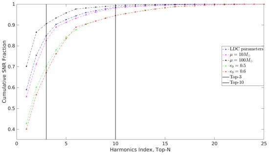
Figure 1.
Cumulative SNR fractions over harmonics in descending order for the 5 signal parameters in Table 1.
The nested inner maximization over the initial angles, , , , is carried out using the Simplex algorithm of Nelder and Mead [64], which has guaranteed convergence to a local maximum. This is found to be quite effective because the 13-dimensional LLR varies much more slowly over the initial angles compared to, for example, the six parameters related to the ODEs. Consequently, as illustrated in Figure 2, the 13-dimensional LLR usually contains only a few peaks over the 3-dimensional space of the initial angles that are, moreover, equal or comparable in magnitude to the highest peak. Thus, to find the maximum value over the initial angles, it is sufficient to use a local maximizer to converge to any one of these local peaks. To ensure that we obtain the value of the global maximum within the 3-dimensional space, we use a grid of 32 different starting points for the local maximization (e.g., for , and for ) and select the best solution.
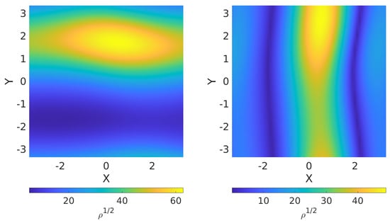
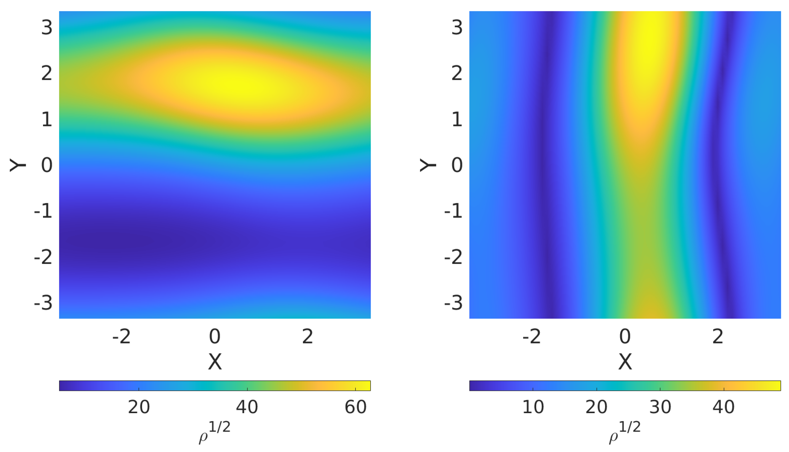
Figure 2.
Illustrations of the peak structure of the function using two 2-dimensional planar cross-sections of the 3-dimensional space formed by the three initial angles. The plane on the left is and the plane on the right is . The X and Y axes lie in these planes and the range along both is . Other planes exhibit similar patterns as above. The figure is produced using the noise realization in LDC-1.2 [58] data and an arbitrary injected signal.
Although numerical maximization over the initial angles incurs additional computation compared to the more restrictive analytical approach outlined in Section 3, its cost is reduced considerably by optimizing the code implementation as follows. The key idea is to apply the TDI linear decomposition in Equation (29) to separate the parameters , , from the inner product and . Thus, we have
where N is the number of harmonics involved and the parameters , , are absorbed in the linear coefficients , . For a given , precomputing the inner products and in the above expressions allows significant savings in computational cost when using a local maximizer over the three initial angles, since they appear only in the set of coefficients . Further savings are obtained by neglecting the off-diagonal inner products above between different harmonics, which tend to be very small. In addition, OpenMP is used to parallelize and speed up the evaluation of the inner products. As a result of the above optimizations, the computational cost of each run of the local maximization is on the millisecond scale using a GHz 8-core processor, which is negligible compared to the time (on the order of seconds) taken by the other steps in the algorithm.
4. Particle Swarm Optimization
The maximization of the LLR over the 10 parameters left over after (a) analytical maximization over A and (b) local maximization over the initial angles must be carried out numerically. As discussed earlier, we use PSO for this step. A brief review of the PSO algorithm is provided below.
PSO is a nature-inspired optimization algorithm inspired by the social behavior of birds and fish, where individuals in a group coordinate their movements to find the best solution to an optimization problem. PSO has been successfully applied in various fields, including engineering, finance, and machine learning.
The PSO algorithm solves the optimization problem
where the function to be maximized is called the fitness function and the space is called the search space. (The fitness function in our case is the 10-dimensional LLR.) This is accomplished in PSO using a set of particles exploring the search space iteratively, where a particle is simply a location in . Each particle represents a potential solution to the optimization problem, and its movement is influenced by both its own experience and the experiences of its neighboring particles.
The dynamics of a particle in PSO is governed by the following equations (with t representing an iteration). The position of a particle is updated following the rule
where is the position of particle i at time t, and is the displacement (called velocity in PSO) update at time . The starting positions and velocities of the particles are commonly picked randomly from a uniform distribution over . Using to denote the j-th component of a vector , the velocity is updated following the rule
where w is the inertia weight, and are acceleration coefficients, and are uniformly distributed random variables between 0 and 1, is the best position of particle i so far (called its personal best or pbest), and is the best position in the entire swarm so far (called the global best or gbest). Here, a position is better than another if its corresponding fitness value is higher. The inertia weight determines the influence of the previous velocity on the current velocity. The corresponding term in the dynamical equation promotes the exploration of the search space by a particle. A common choice is to use a linearly decreasing inertia weight over iterations. The acceleration coefficients control the attraction strengths of the personal best () and global best () on the movement of the particle. A typical setting is . These terms promote the convergence of the algorithm towards previously identified good solutions. In addition to these parameters, it is necessary to constrain the velocities of particles in order to prevent the entire swarm from quickly leaving the search space. The velocity is commonly constrained by a parameter called the maximum velocity, , with enforced for all iterations.
Before updating the velocity of a particle, the pbest of all particles and the gbest are updated following
and
In addition to the parameters listed above, one must set some hyperparameters in the PSO algorithm. These include the number of particles and the form of the initial and boundary conditions. We use the so-called let-them-fly boundary condition, in which no changes are made to the position or velocity of a particle that leaves the search space but its fitness is set to . Gradually, since the pbest and gbest are always located inside the search space, the particle is drawn back in by their attractive forces. The number of particles in the swarm influences the algorithm’s exploration and convergence. A small swarm cannot efficiently explore a high-dimensional space, while a larger swarm size may prematurely converge to a local maximum before the particles have had time to fully explore the search space. Empirical evidence suggests that having about 40 particles works well in most cases, and this is the number adopted in this paper to obtain our main results. Finally, one must set up a termination criterion, and a common one that is also adopted in this paper is reaching a predefined number, , of iterations.
There are several variations around the basic PSO algorithm described above that seek to achieve different trade-offs between the exploration and exploitation (i.e., convergence) phases of the search. Delaying the onset of the exploitation phase leads to a higher computational cost for the search but also improves the chances of finding the global maximum due to a more thorough exploration of the search space. One such variant of PSO, and the one that is used in this paper, is Local Best PSO, which introduces the concept of local best (lbest) positions, , to replace gbest in the velocity update equation. The lbest position is defined by
where is a set of particle indices called the neighborhood of particle i. The scheme used to set up is called the swarm topology. Note that if is set to be the entire swarm for each i, one recovers the gbest PSO described earlier. In this paper, we use the so-called ring topology, in which the particle indices are arranged on a closed circle and the neighborhood of each particle is the set of adjacent indices on both sides. For example, in our case, we set the neighborhood size to 3, which means that only the particles immediately adjacent on either side constitute the neighborhood of a given particle. By using lbest instead of gbest in the velocity update equation, the information about the latter propagates only indirectly, through neighbors, and more slowly through the swarm. This extends the exploration phase of the search, generally leading to better performance for more rugged fitness functions.
To boost the performance of PSO, or any stochastic optimization algorithm, a straightforward approach is to carry out parallel runs of PSO with independent pseudorandom number streams, where depends on the specific computational resources at hand, and to choose the final solution to be the one from the run that finds the best fitness value. If the probability of any one run succeeding in a specified region around the global maximum is p, the probability that all independent runs will fail to converge, , drops exponentially quickly with increasing . Thus, one can tune PSO to perform moderately well in any one run and simply use the parallel runs strategy to obtain significantly better overall performance.
For parametric inference problems, such as the one being considered here, there exists [44] an objective strategy for the tuning of PSO. This is carried out using simulated data realizations, each containing the same true signal. If PSO is successful in locating the global maximum of the fitness function in a given realization, the fitness value that it finds must be higher than the value at the location of the true signal in the search space. Hence, one can measure the fraction of realizations in which this condition is satisfied. The higher this fraction, the better tuned the PSO is. In most cases, the tuning process involves searching over combinations of and alone, keeping all other PSO parameters fixed. We provide more details about the choice of and in Section 5.
5. Results
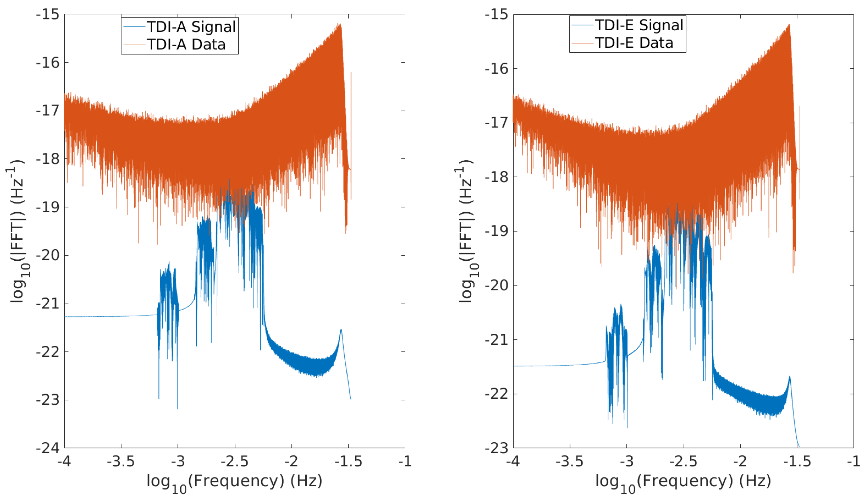
Given the computational resources available to us and the current level of parallelization used in our code, we have limited our analysis to year data in this paper. For similar reasons, the same duration has been used widely in other studies [36,65,66] for the exploration of EMRI data analysis methods. We have used the LDC-1.2 [58] signal as our injected signal but adjust the SNR to have three different values, , by setting the distance D to Gpc, Gpc, and Gpc, respectively. As a result, our injected signal has the same source parameters, given in Table 2, as used in LDC-1.2 [58], except the distance. The noise realization in the data analyzed here was obtained as the difference between the data and the signal provided in LDC-1.2 [58]. Thus, both our injected signal and the noise realization are identical to the ones used in LDC-1.2 [58], except for (a) distance scaling and (b) the reduction of the data duration from 2 years to 6 months. Figure 3 shows the data and the injected signal with in the Fourier domain for the TDI A and E combinations. We see that, at this SNR, the signal is quite weak in the Fourier domain relative to the noise.
Table 2.
The injected source parameters and range width used in our search. Currently, the location of the injected signal is set at the center of the given range. We leave a more general search, with injected signals placed non-centrally in the search space, to future work.
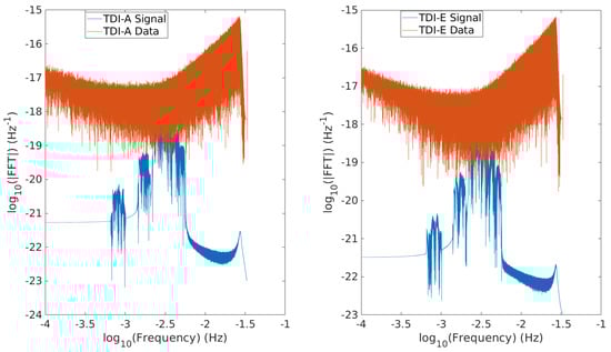
Figure 3.
Magnitudes of the FFTs of the injected signal with in blue and the corresponding data in red, where the TDI A combination is illustrated in the left panel and the TDI E combination is displayed in the right panel. See their definitions in Equation (1).
We carry out the 10-dimensional PSO search with the search ranges for the signal parameters set to the values given in Table 2. The search range for a given parameter is expressed as a multiple of , where is the CRLB on the estimation error for that parameter at the specified signal SNR. Thus, it is important to note that the search range expands with the lowering of the SNR since this increases . In effect, since a lower SNR and larger search range make it more difficult to locate the global maximum, the strength of the challenge posed to the data analysis method is controlled in this study using the SNR as a parameter.
Following the strategy outlined in Section 4, there are two primary tunable hyperparameters for our PSO-based search, the number of independent runs of PSO and the number of iterations, , per run. However, due to the limitations of the computational resources, we carried out the very coarse tuning of these parameters based on a small set of runs and set = 10,000 and . Moreover, we were unable to run all 6 runs in parallel and had to carry them out serially. In order to save computational resources, we terminated the sequence of runs once, as explained in Section 4; a successful one appeared in which the fitness value exceeded that at the true location. As a result, the actual was 3, 1, 3 for , respectively. It is important to note that since we did not choose the best of 6 runs, we may not have obtained the best possible fitness values.
The results obtained from the 10-dimensional search applied to the three data realizations described above are summarized in Table 3. We also report the square root of the fitness values, which provide the estimated SNRs, at the true signal location for both the 13-dimensional fitness function, given by Equation (26) and the 10-dimensional one (c.f., Section 3.2), in which the three initial angles are maximized over numerically using the Nelder–Mead method. Since the global maximum over the three initial angles always shifts from their true values due to noise in the data, the 10-dimensional search always finds a better estimated SNR, as observed. Further details regarding Table 3 are noted below.
Table 3.
Outputs from the PSO searches for different injected signal SNRs. For each of the 6 ODE-related parameters, we show two numbers (with denoting the standard deviation): (top) the difference between the estimated and true parameter values relative to the FIM error for that parameter, and (bottom) the corresponding FIM error. Further details regarding the table are discussed in Section 5.
- As noted above, one expects a successful PSO search to find a 10-dimensional fitness value that is larger than the one at the true location. We show the corresponding estimated SNR from the successful run in bold.
- The parameter estimation errors listed in the table are evaluated based on the best-fit locations of the successful PSO search. For the parameters , M, , , , and , we show their estimation errors, defined as the difference between the true and best-fit values, relative to their respective CRLB errors (evaluated at the true location), while the error is shown relative to its true value for D. For the parameters , , , and , we simply show the error itself.
- Having obtained the 10-dimensional best-fit location of the successful PSO search, which uses templates restricted to the 10 loudest harmonics, we rerun the 3-dimensional local maximization at this location using all 25 harmonics to estimate the three initial angles, , , . This is done to reveal the influence of the weak harmonics beyond the loudest 10 on the initial angles. The estimated initial angles are then used in the estimation of the distance D using Equation (27).
- With the 14-dimensional recovered parameters in hand, the estimated TDI A and E signals can be obtained by rerunning Equations (2) and (1). The overlap between the estimated A and E signals and the corresponding true signals, computed separately and in combination as defined in Equation (15), are reported as the quantities , , and .
We see from Table 3 that the estimated errors of the parameters , M, , , , are within level, parameter D within level, and the angles of sky locations , are within ∼ radians level for all three SNRs. The errors in the parameters , for are larger, which may result from secondary peaks in the fitness, as described in Section 1. As a complementary measure of the performance, we see that the overlaps, both individual and combined, between the estimated and injected signals are ≳, which indicates that the signal waveform was estimated well. We observe that the errors in the parameters related to the ODEs are smaller for the 30 case, despite the higher difficulty of this search, compared to . If this is not a random fluctuation specific to the data realization used, it either indicates the effect of degenerate secondary peaks in the fitness function, which may be more prominent for higher SNR signals and could have attracted PSO, or indicates that our current settings for PSO, governed mainly by computational constraints, may need to be changed to a higher or to stabilize its performance.
6. Discussion
We have demonstrated the first application of PSO to the EMRI search problem and shown that, in the context of a limited search space and reduced data length, it performs well at reasonable SNR levels. Using three different SNRs () and a search space with coordinate ranges limited to for all parameters except for , with being the CRLB standard deviation, PSO was able to successfully find the signal, as shown by the small estimation errors for the parameters that affect the intrinsic phase evolution of the GW signal and the overlaps between the estimated and true signals. This sets the stage for the further exploration of the EMRI search problem using PSO-based strategies. Our study, which is ongoing, also provides useful guidance for hierarchical strategies in terms of the coordinate ranges to which they should seek to constrain the main search.
The main innovation in our approach is the lifting of several restrictions and approximations adopted in other proposed strategies. In particular, we use local numerical maximization over the three initial angles , , , which obviates the need to severely restrict the number of harmonics used in the templates and avoids the issues associated with such restrictions. We only make the reasonable restriction of keeping the 10 loudest harmonics based on their contribution to the total SNR. Allowing 10 harmonics in the templates leads to a more stable SNR contribution, as well as the order of the dominant harmonics across a wider range of parameter values. Implementing certain optimizations in the implementation of the local maximization makes its computational cost insignificant compared to the rest of the code.
Besides the high dimensionality of the search space, the main challenge in the EMRI search is the high degeneracy of the fitness function, with many comparable secondary peaks due to the superposition of multiple harmonics in the waveform. As discussed in [39], characterizing this degeneracy is quite challenging and it is difficult to exploit in a search. One possible approach is to design less degenerate fitness functions by employing [36] surrogate phenomenological EMRI waveforms [34]. Another approach would be to use the fact that, like the initial angles, the parameters and only contribute to the time-independent amplitude of the waveform and use local maximization over them also, following the code optimization discussed in Section 3.2, leaving a potentially easier 8-dimensional search for PSO. Such a lower-dimensional search will be considered in our future work.
A key limitation of our study was the inability to test a much larger number of PSO iterations or runs due to computational resource constraints. While successful in all the cases tested here, PSO exhibited somewhat unstable performance by showing better performance at the lowest SNR that was used. While this could have also been caused by degeneracies in the EMRI fitness function, a better understanding requires much larger PSO runs. The computational resources also limited us from studying the case of signals with weaker SNRs. We have conducted preliminary studies for a much lower SNR of 20 in year of data and found that PSO can still detect the signal by obtaining the square roots of the fitness values (e.g., ≈17), which are well above the ones obtained for pure noise (e.g., ≈10). However, due to the lack of a sufficient number of iterations and runs, PSO tends to converge to secondary maxima most of the time and incurs very large parameter estimation errors. In the future, we will include GPU-based hardware acceleration in our code to alleviate this problem and push the PSO-based search further, using larger runs.
Author Contributions
Conceptualization, S.D.M. and X.-B.Z.; software, X.-B.Z. and S.D.M. (for PSO); validation, X.-B.Z., S.D.M., H.-G.L. and Y.-X.L.; writing—original draft preparation, X.-B.Z.; writing—review and editing, S.D.M., H.-G.L. and Y.-X.L.; supervision, S.D.M. and H.-G.L.; project administration, Y.-X.L.; funding acquisition, H.-G.L. and Y.-X.L. All authors have read and agreed to the published version of the manuscript.
Funding
The work of X.-B.Z., H.-G.L., and Y.-X.L. was supported by the following grants: (1) the National Key Research and Development Program of China (grant No. 2021YFC2203003); (2) the National Key Research and Development Program of China (grant No. 2022YFA1402704); (3) the National Natural Science Foundation of China (NSFC) (Grant No. 11834005 and No. 12247101).
Data Availability Statement
The LDC data used in this study are publicly available from https://lisa-ldc.lal.in2p3.fr/challenge1 accessed on 13 February 2024. The PSO code used in this study is based on that provided in the GitHub repository RAAPTR, available at https://github.com/yanwang2012/RAAPTR, accessed on 13 February 2024. The rest of the code simply implements the mathematical formalisms for GLRT and MLE described in this paper, with all necessary details provided to aid reproducibility.
Acknowledgments
The computations were performed on the high-performance computers of the State Key Laboratory of Scientific and Engineering Computing, Chinese Academy of Sciences. We express our gratitude to RunQiu Liu for granting us access to the cluster and providing invaluable suggestions for our research. We also extend our appreciation to the administrator, Yin Qian, for assisting us in utilizing the cluster effectively. Furthermore, we would like to acknowledge the insightful discussions that we had with Xian Chen, Wen-biao Han, Peng Xu, Wen-lin Tang, Qun-ying Xie, Xue-hao Zhang, Shao-dong Zhao, Yi-yang Guo, Han-zhi Wang, Shu-zhu Jin, Qian-yun Yun, and Hou-qiang Teng.
Conflicts of Interest
The authors declare no conflicts of interest. The funders had no role in the design of the study; in the collection, analyses, or interpretation of data; in the writing of the manuscript; or in the decision to publish the results.
Abbreviations
The following abbreviations are used in this manuscript:
| AK | Analytical Kludge |
| CO | Compact Object |
| CRLB | Cramer–Rao Lower Bound |
| DFT | Discrete Fourier Transform |
| EMRI | Extreme Mass Ratio Inspiral |
| FIM | Fisher Information Matrix |
| GW | Gravitational Wave |
| GLRT | Generalized Likelihood Ratio Test |
| GPU | Graphics Processing Unit |
| LDC | LISA Data Challenge |
| LLR | Log-Likelihood Ratio |
| LISA | Laser Interferometer Space Antenna |
| MLE | Maximum Likelihood Estimation |
| MCMC | Markov Chain Monte Carlo |
| MLDC | Mock LISA Data Challenge |
| MBH | Massive Black Hole |
| MPI | Message Passing Interface |
| ODE | Ordinary Differential Equation |
| PSD | Power Spectral Density |
| PSO | Particle Swarm Optimization |
| SNR | Signal-to-Noise Ratio |
| SSB | Solar System Barycenter |
| SI | Swarm Intelligence |
| TDI | Time Delay Interferometry |
References
- Amaro-Seoane, P.; Audley, H.; Babak, S.; Baker, J.; Barausse, E.; Bender, P.; Berti, E.; Binetruy, P.; Born, M.; Bortoluzzi, D.; et al. Laser Interferometer Space Antenna. arXiv 2017, arXiv:1702.00786. [Google Scholar]
- Hu, W.R.; Wu, Y.L. The Taiji Program in Space for gravitational wave physics and the nature of gravity. Natl. Sci. Rev. 2017, 4, 685–686. [Google Scholar] [CrossRef]
- Luo, Z.; Guo, Z.; Jin, G.; Wu, Y.; Hu, W. A brief analysis to Taiji: Science and technology. Results Phys. 2020, 16, 102918. [Google Scholar] [CrossRef]
- Luo, J.; Chen, L.S.; Duan, H.Z.; Gong, Y.G.; Hu, S.; Ji, J.; Liu, Q.; Mei, J.; Milyukov, V.; Sazhin, M.; et al. TianQin: A space-borne gravitational wave detector. Class. Quantum Gravity 2016, 33, 035010. [Google Scholar] [CrossRef]
- Nelemans, G.; Yungelson, L.R.; Zwart, S.F.P. The gravitational wave signal from the galactic disk population of binaries containing two compact objects. Astron. Astrophys. 2001, 375, 890–898. [Google Scholar] [CrossRef]
- Korol, V.; Rossi, E.M.; Groot, P.J.; Nelemans, G.; Toonen, S.; Brown, A.G.A. Prospects for detection of detached double white dwarf binaries with Gaia, LSST and LISA. Mon. Not. R. Astron. Soc. 2017, 470, 1894–1910. [Google Scholar] [CrossRef]
- Korol, V.; Hallakoun, N.; Toonen, S.; Karnesis, N. Observationally driven Galactic double white dwarf population for LISA. Mon. Not. R. Astron. Soc. 2022, 511, 5936–5947. [Google Scholar] [CrossRef]
- Barausse, E.; Bellovary, J.; Berti, E.; Holley-Bockelmann, K.; Farris, B.; Sathyaprakash, B.; Sesana, A. Massive Black Hole Science with eLISA. J. Phys. Conf. Ser. 2015, 610, 012001. [Google Scholar] [CrossRef]
- Klein, A.; Barausse, E.; Sesana, A.; Petiteau, A.; Berti, E.; Babak, S.; Gair, J.; Aoudia, S.; Hinder, I.; Ohme, F.; et al. Science with the space-based interferometer eLISA: Supermassive black hole binaries. Phys. Rev. D 2016, 93, 024003. [Google Scholar] [CrossRef]
- Wang, H.T.; Jiang, Z.; Sesana, A.; Barausse, E.; Huang, S.J.; Wang, Y.F.; Feng, W.F.; Wang, Y.; Hu, Y.M.; Mei, J.; et al. Science with the TianQin observatory: Preliminary results on massive black hole binaries. Phys. Rev. D 2019, 100, 043003. [Google Scholar] [CrossRef]
- Gair, J.R.; Barack, L.; Creighton, T.; Cutler, C.; Larson, S.L.; Phinney, E.S.; Vallisneri, M. Event rate estimates for LISA extreme mass ratio capture sources. Class. Quantum Gravity 2004, 21, S1595–S1606. [Google Scholar] [CrossRef]
- Babak, S.; Gair, J.; Sesana, A.; Barausse, E.; Sopuerta, C.F.; Berry, C.P.L.; Berti, E.; Amaro-Seoane, P.; Petiteau, A.; Klein, A. Science with the space-based interferometer LISA. V: Extreme mass-ratio inspirals. Phys. Rev. D 2017, 95, 03012. [Google Scholar] [CrossRef]
- Gair, J.R.; Babak, S.; Sesana, A.; Amaro-Seoane, P.; Barausse, E.; Berry, C.P.L.; Berti, E.; Sopuerta, C. Prospects for observing extreme-mass-ratio inspirals with LISA. J. Phys. Conf. Ser. 2017, 840, 012021. [Google Scholar] [CrossRef]
- Fan, H.M.; Hu, Y.M.; Barausse, E.; Sesana, A.; Zhang, J.d.; Zhang, X.; Zi, T.G.; Mei, J. Science with the TianQin observatory: Preliminary result on extreme-mass-ratio inspirals. Phys. Rev. D 2020, 102, 063016. [Google Scholar] [CrossRef]
- Vázquez-Aceves, V.; Zwick, L.; Bortolas, E.; Capelo, P.R.; Amaro-Seoane, P.; Mayer, L.; Chen, X. Revised event rates for extreme and extremely large mass-ratio inspirals. Mon. Not. R. Astron. Soc. 2022, 510, 2379–2390. [Google Scholar] [CrossRef]
- Littenberg, T.; Cornish, N.; Lackeos, K.; Robson, T. Global Analysis of the Gravitational Wave Signal from Galactic Binaries. Phys. Rev. D 2020, 101, 123021. [Google Scholar] [CrossRef]
- Littenberg, T.B.; Cornish, N.J. Prototype global analysis of LISA data with multiple source types. Phys. Rev. D 2023, 107, 063004. [Google Scholar] [CrossRef]
- Zhang, X.; Mohanty, S.D.; Zou, X.; Liu, Y. Resolving Galactic binaries in LISA data using particle swarm optimization and cross-validation. Phys. Rev. D 2021, 104, 024023. [Google Scholar] [CrossRef]
- Zhang, X.H.; Zhao, S.D.; Mohanty, S.D.; Liu, Y.X. Resolving Galactic binaries using a network of space-borne gravitational wave detectors. Phys. Rev. D 2022, 106, 102004. [Google Scholar] [CrossRef]
- Strub, S.H.; Ferraioli, L.; Schmelzbach, C.; Stähler, S.C.; Giardini, D. Bayesian parameter estimation of Galactic binaries in LISA data with Gaussian process regression. Phys. Rev. D 2022, 106, 062003. [Google Scholar] [CrossRef]
- Strub, S.H.; Ferraioli, L.; Schmelzbach, C.; Stähler, S.C.; Giardini, D. Accelerating global parameter estimation of gravitational waves from Galactic binaries using a genetic algorithm and GPUs. Phys. Rev. D 2023, 108, 103018. [Google Scholar] [CrossRef]
- Babak, S.; Baker, J.G.; Benacquista, M.J.; Cornish, N.J.; Crowder, J.; Larson, S.L.; Plagnol, E.; Porter, E.K.; Vallisneri, M.; Vecchio, A.; et al. The Mock LISA Data Challenges: From Challenge 1B to Challenge 3. Class. Quantum Gravity 2008, 25, 184026. [Google Scholar] [CrossRef]
- Babak, S.; Baker, J.G.; Benacquista, M.J.; Cornish, N.J.; Larson, S.L.; Mendel, I.; McWilliams, S.T.; Petiteau, A.; Porter, E.K.; Robinson, E.L.; et al. The Mock LISA Data Challenges: From Challenge 3 to Challenge 4. Class. Quantum Gravity 2010, 27, 084009. [Google Scholar] [CrossRef]
- Baghi, Q. The LISA Data Challenges. arXiv 2022, arXiv:2204.12142. [Google Scholar]
- Ren, Z.; Zhao, T.; Cao, Z.; Guo, Z.K.; Han, W.B.; Jin, H.B.; Wu, Y.L. Taiji data challenge for exploring gravitational wave universe. Front. Phys. 2023, 18, 64302. [Google Scholar] [CrossRef]
- Gair, J.R.; Mandel, I.; Wen, L. Improved time-frequency analysis of extreme-mass-ratio inspiral signals in mock LISA data. Class. Quantum Gravity 2008, 25, 184031. [Google Scholar] [CrossRef]
- Barack, L.; Cutler, C. LISA capture sources: Approximate waveform, signal-to-noise ratios, and parameter estimation accuracy. Phys. Rev. D 2004, 69, 082005. [Google Scholar] [CrossRef]
- Peters, P.C.; Mathews, J. Gravitational radiation from point masses in a Keplerian orbit. Phys. Rev. 1963, 131, 435–439. [Google Scholar] [CrossRef]
- Peters, P.C. Gravitational Radiation and the Motion of Two Point Masses. Phys. Rev. 1964, 136, B1224–B1232. [Google Scholar] [CrossRef]
- Kay, S.M. Fundamentals of Statistical Signal Processing; Prentice Hall: Hoboken, NJ, USA, 1993; Volumes 1 & 2. [Google Scholar]
- Liu, J.S. Monte Carlo Strategies in Scientific Computing; Springer: Berlin/Heidelberg, Germany, 2008. [Google Scholar]
- Babak, S.; Gair, J.R.; Porter, E.K. An Algorithm for detection of extreme mass ratio inspirals in LISA data. Class. Quantum Gravity 2009, 26, 135004. [Google Scholar] [CrossRef]
- Cornish, N.J. Detection Strategies for Extreme Mass Ratio Inspirals. Class. Quantum Gravity 2011, 28, 094016. [Google Scholar] [CrossRef]
- Wang, Y.; Shang, Y.; Babak, S.; Shang, Y.; Babak, S. EMRI data analysis with a phenomenological waveform. Phys. Rev. D 2012, 86, 104050. [Google Scholar] [CrossRef]
- Bandopadhyay, D.; Moore, C.J. LISA stellar-mass black hole searches with semicoherent and particle-swarm methods. Phys. Rev. D 2023, 108, 084014. [Google Scholar] [CrossRef]
- Ye, C.Q.; Fan, H.M.; Torres-Orjuela, A.; Zhang, J.d.; Hu, Y.M. Identification of Gravitational-waves from Extreme Mass Ratio Inspirals. arXiv 2023, arXiv:2310.03520. [Google Scholar]
- Ali, A. Bayesian Inference on EMRI Signals in LISA Data. Available online: https://researchspace.auckland.ac.nz/handle/2292/7123 (accessed on 14 February 2024).
- Ali, A.; Christensen, N.; Meyer, R.; Rover, C. Bayesian inference on EMRI signals using low frequency approximations. Class. Quantum Gravity 2012, 29, 145014. [Google Scholar] [CrossRef]
- Chua, A.J.K.; Cutler, C.J. Nonlocal parameter degeneracy in the intrinsic space of gravitational-wave signals from extreme-mass-ratio inspirals. Phys. Rev. D 2022, 106, 124046. [Google Scholar] [CrossRef]
- Arnaud, K.A.; Babak, S.; Baker, J.G.; Benacquista, M.J.; Cornish, N.J.; Cutler, C.; Finn, L.S.; Larson, S.L.; Littenberg, T.; Porter, E.K.; et al. An Overview of the second round of the Mock LISA Data Challenges. Class. Quantum Gravity 2007, 24, S551–S564. [Google Scholar] [CrossRef]
- Kennedy, J.; Eberhart, R.C. Particle swarm optimization. In Proceedings of the International Conference on Neural Networks, Perth, WA, Australia, 27 November–1 December 1995; pp. 1942–1948. [Google Scholar]
- Bratton, D.; Kennedy, J. Defining a Standard for Particle Swarm Optimization. In Proceedings of the 2007 IEEE Swarm Intelligence Symposium, Honolulu, HI, USA, 1–5 April 2007; pp. 120–127. [Google Scholar] [CrossRef]
- Mohanty, S.D. Swarm Intelligence Methods for Statistical Regression; CRC Press: Boca Raton, FL, USA, 2018. [Google Scholar] [CrossRef]
- Wang, Y.; Mohanty, S.D. Particle Swarm Optimization and gravitational wave data analysis: Performance on a binary inspiral testbed. Phys. Rev. D 2010, 81, 063002. [Google Scholar] [CrossRef]
- Weerathunga, T.S.; Mohanty, S.D. Performance of Particle Swarm Optimization on the fully-coherent all-sky search for gravitational waves from compact binary coalescences. Phys. Rev. D 2017, 95, 124030. [Google Scholar] [CrossRef]
- Normandin, M.E.; Mohanty, S.D.; Weerathunga, T.S. Particle Swarm Optimization based search for gravitational waves from compact binary coalescences: Performance improvements. Phys. Rev. D 2018, 98, 044029. [Google Scholar] [CrossRef]
- Normandin, M.E.; Mohanty, S.D. Towards a real-time fully-coherent all-sky search for gravitational waves from compact binary coalescences using particle swarm optimization. Phys. Rev. D 2020, 101, 082001. [Google Scholar] [CrossRef]
- Wang, Y.; Mohanty, S.D.; Jenet, F.A. A coherent method for the detection and estimation of continuous gravitational wave signals using a pulsar timing array. Astrophys. J. 2014, 795, 96. [Google Scholar] [CrossRef]
- Wang, Y.; Mohanty, S.D.; Jenet, F.A. Coherent network analysis for continuous gravitational wave signals in a pulsar timing array: Pulsar phases as extrinsic parameters. Astrophys. J. 2015, 815, 125. [Google Scholar] [CrossRef]
- Zhu, X.; Wen, L.; Xiong, J.; Xu, Y.; Wang, Y.; Mohanty, S.D.; Hobbs, G.; Manchester, R.N. Detection and localization of continuous gravitational waves with pulsar timing arrays: The role of pulsar terms. Mon. Not. R. Astron. Soc. 2016, 461, 1317–1327. [Google Scholar] [CrossRef]
- Wang, Y.; Mohanty, S.D. Pulsar Timing Array Based Search for Supermassive Black Hole Binaries in the Square Kilometer Array Era. Phys. Rev. Lett. 2017, 118, 151104, Erratum in Phys. Rev. Lett. 2020, 124, 169901. [Google Scholar] [CrossRef] [PubMed]
- Wang, Y.; Mohanty, S.D.; Qian, Y.Q. Continuous gravitational wave searches with pulsar timing arrays: Maximization versus marginalization over pulsar phase parameters. J. Phys. Conf. Ser. 2017, 840, 012058. [Google Scholar] [CrossRef]
- Qian, Y.Q.; Mohanty, S.D.; Wang, Y. Iterative time-domain method for resolving multiple gravitational wave sources in pulsar timing array data. Phys. Rev. D 2022, 106, 023016. [Google Scholar] [CrossRef]
- Mohanty, S.D. Spline Based Search Method For Unmodeled Transient Gravitational Wave Chirps. Phys. Rev. D 2017, 96, 102008. [Google Scholar] [CrossRef]
- Mohanty, S.D.; Fahnestock, E. Adaptive spline fitting with particle swarm optimization. Comput. Stat. 2021, 36, 155–191. [Google Scholar] [CrossRef]
- Mohanty, S.D.; Chowdhury, M.A.T. Glitch subtraction from gravitational wave data using adaptive spline fitting. Class. Quantum Gravity 2023, 40, 125001. [Google Scholar] [CrossRef]
- Tinto, M.; Dhurandhar, S.V. Time Delay. Living Rev. Rel. 2005, 8, 4. [Google Scholar] [CrossRef]
- LISA Data Challenge, Code and Maunal. Available online: https://lisa-ldc.lal.in2p3.fr/challenge1; https://lisa-ldc.lal.in2p3.fr/static/data/pdf/LDC-manual-002.pdf (accessed on 13 February 2024).
- Babak, S.; Petiteau, A.; Hewitson, M. LISA Sensitivity and SNR Calculations. arXiv 2021, arXiv:2108.01167. [Google Scholar]
- Press, W.H.; Teukolsky, S.A.; Vetterling, W.T.; Flannery, B.P. Numerical Recipes in Fortran 90: The Art of Parallel Scientific Computing, 2nd ed.; Fortran Numerical Recipes 2; Cambridge University Press: Cambridge, UK, 1996. [Google Scholar]
- OpenMP. Available online: https://www.openmp.org/ (accessed on 13 February 2024).
- Jaranowski, P.; Krolak, A.; Schutz, B.F. Data analysis of gravitational - wave signals from spinning neutron stars. 1. The Signal and its detection. Phys. Rev. D 1998, 58, 063001. [Google Scholar] [CrossRef]
- Robson, T.; Cornish, N.J.; Liu, C. The construction and use of LISA sensitivity curves. Class. Quantum Gravity 2019, 36, 105011. [Google Scholar] [CrossRef]
- The gsl Library. Available online: https://www.gnu.org/software/gsl/doc/html/multimin.html (accessed on 13 February 2024).
- Yun, Q.; Han, W.B.; Guo, Y.Y.; Wang, H.; Du, M. Detecting extreme-mass-ratio inspirals for space-borne detectors with deep learning. arXiv 2023, arXiv:2309.06694. [Google Scholar]
- Yun, Q.; Han, W.B.; Guo, Y.Y.; Wang, H.; Du, M. The detection, extraction and parameter estimation of extreme-mass-ratio inspirals with deep learning. arXiv 2023, arXiv:2311.18640. [Google Scholar]
Disclaimer/Publisher’s Note: The statements, opinions and data contained in all publications are solely those of the individual author(s) and contributor(s) and not of MDPI and/or the editor(s). MDPI and/or the editor(s) disclaim responsibility for any injury to people or property resulting from any ideas, methods, instructions or products referred to in the content. |
© 2024 by the authors. Licensee MDPI, Basel, Switzerland. This article is an open access article distributed under the terms and conditions of the Creative Commons Attribution (CC BY) license (https://creativecommons.org/licenses/by/4.0/).