Photometry and Models of Seven Main-Belt Asteroids

Abstract

The China Near-Earth Object Survey Telescope (CNEOST) conducted four photometric surveys from 2015 to 2018 using image processing and aperture photometry techniques to obtain extensive light curve data on asteroids. The second-order Fourier series method was selected for its efficiency in determining the rotation periods of the observed asteroids. Our study successfully derived rotation periods for 892 asteroids, with 648 of those matching values recorded in the LCDB (for asteroids with U > 2). To enhance the reliability of the derived spin parameters and shape models, we also amassed a comprehensive collection of published light curve data supplemented by additional photometric observations on a targeted subset of asteroids conducted using multiple telescopes between 2021 and 2022. Through the application of convex inversion techniques, we successfully derived spin parameters and shape models for seven main-belt asteroids (MBAs): (2233) Kuznetsov, (2294) Andronikov, (2253) Espinette, (4796) Lewis, (1563) Noel, (2912) Lapalma, and (5150) Fellini. Our thorough analysis identified two credible orientations for the rotational poles of these MBAs, shedding light on the prevalent issue of “ambiguity in pole direction” that often accompanies photometric inversion processes. CNEOST continues its observational endeavors, and future collected data combined with other independent photometric measurements will facilitate further inversion to better constrain the spin parameters and yield more refined shape models.

1. Introduction

Asteroids have undergone a multitude of physical processes throughout their evolutionary history, including collisions, mergers, fission, and migration of surface materials. Consequently, their current rotational states and shapes differ markedly from their initial formation stages [1,2,3]. Inversion studies of asteroids offer valuable insights into their evolutionary trajectories as well as the broader history of the solar system. Presently, asteroids are a primary focus of deep space exploration missions, with preliminary inversion studies of target asteroids providing crucial data that can inform these missions. For instance, Nolan et al. [4] conducted inversion studies on the target asteroid (101955) Bennu prior to the OSIRIS-REx mission, while Li and Scheeres [5] completed an inversion study of the asteroid (469219) 2016 HO3. The ongoing deep space mission targeting (469219) 2016 HO3 stands to benefit significantly from data derived through shape inversion and surface environmental studies. Currently, photometric data are the most widely utilized and frequently employed in asteroid shape inversion research, particularly data from ground-based observations. In contrast, alternative imaging methods, including radar images, occultations, and adaptive optics (AO) images are still underutilized. Expanding the incorporation of these imaging techniques may further enrich the data landscape for asteroid shape inversion studies.

Most asteroids with established shape models can be accessed via the Database of Asteroid Models from Inversion Techniques 1 [6]. The convex light curve inversion method has been mathematically proven to converge to a unique solution only when the convexity hypothesis is upheld [7,8]. While this method is limited in its ability to describe concave structures of asteroids, numerous instances demonstrate that the convex shape model serves as a close approximation of the convex hull of the asteroid’s actual shape [8]. Furthermore, Kaasalainen and Ďurech [9] highlighted that even a modest number of light curves (fewer than ten) derived from diverse geometries can yield sufficient information to construct a unique model. Thus, this method stands as a powerful tool for reconstructing shape models of asteroids within the Solar System. Accordingly, expanding the sample size of asteroids with reliable spin parameters and shape models remains a pivotal objective in the field of planetary science.

In line with this objective, the present work aims to use photometric data obtained from the China Near-Earth Object Survey Telescope (CNEOST) to derive rotation periods and reconstruct the fundamental shapes of asteroids. The CNEOST functions as a sky survey that maps the population of asteroids, including near-Earth asteroids (NEAs), with a primary focus on detecting potentially hazardous NEAs. In addition to its astrometric measurements used for asteroid orbit determination, the CNEOST conducts extensive photometric surveys to measure asteroid brightness. During these surveys, the telescope achieves a limiting magnitude of approximately 20.1 mag in the R band and 19.9 mag in the I band, utilizing exposure times of 90 s.

This article primarily presents an analysis of the photometric data collected from the CNEOST, specifically detailing the reconstruction of shape models for seven main-belt asteroids (MBAs). The study integrates the CNEOST photometry with other independent datasets. Section 2 provides a comprehensive description of the CNEOST lightcurve dataset from 2015 to 2018, in addition to published datasets and new photometric observations from 2021 to 2022, along with detailed information about the data sources, telescopes, and data reduction processes employed. Section 3 concentrates on the data analysis, offering an in-depth overview of the analytical method and the convex light curve inversion techniques used throughout the study. Section 4 outlines the inversion results for the seven MBAs, while Section 5 summarizes these results.

2. Observational Data

2.1. Instruments and Sites

Between 2015 and 2018, four photometric surveys were conducted using the CNEOST [10], during which CCD images were captured utilizing the Bessel R filter in 2015, 2016, and 2017 and the Bessel I filter in 2018. Our analysis is primarily based on the photometric observation data obtained from the Purple Mountain Observatory’s CNEOST2. A significant number of light curves were generated for the observed asteroids, with most subjects being observed continuously for two to five nights during their respective apparitions.

In addition to the CNEOST, our photometric observations encompassed five different telescopes and sites. Notably, observations of several MBAs among the seven target asteroids were conducted in May 2021 using a 0.4 m telescope located at Ali, China. Further observations of the seven MBAs were performed between May and November 2022 at Yaoan Observatory, Abastumani Observatory, and the Cerro Tololo Inter-American Observatory. The subsequent list provides detailed information about these telescopes and their respective observing equipment:

• The CNEOST is a Schmidt telescope system featuring a 1.2 m primary mirror complemented by a 1.04 m corrector. It operates with a focal ratio of $f/1.8$ and is equipped with an STA1600LN CCD detector (Semiconductor Technology Associates, Inc., San Clemente, CA, USA), which delivers a resolution of 10,000 × 10,000 pixels, resulting in an FOV of $3.{02}^{\circ }\times 3.{02}^{\circ }$.
• The Yaoan High Precision Telescope (YAHPT) is a 0.8 m telescope located at Yaoan Station in China. It has a focal length of 8 m and is fitted with a 2048 × 2048 PI camera. This configuration provides an FOV of $11.8^{\prime }\times 11.8^{\prime }$ with a pixel scale of $0.{347}^{\prime \prime }\times 0.{347}^{\prime \prime }$. For this telescope, CCD images were captured using the Bessel V filter from July to October 2022, followed by observations with the Rc filter in November 2022.
• A 0.7 m Maksutov system mirror telescope utilized at Abastumani Observatory [11] possesses a focal length of 2.46 m and is equipped with a PL4240 CCD (Finger Lakes Instrumentation, Lima, NY, USA), yielding an FOV of ${30}^{\prime }\times {30}^{\prime }$. Photometric observations with this telescope were conducted using the Bessel V filter.
• A 0.8 m telescope at Cerro Tololo Inter-American Observatory3 is outfitted with an FLI ML16803 camera (Finger Lakes Instrumentation, Lima, NY, USA) with a resolution of 4096 × 4096 pixels, providing an FOV of ${23}^{\prime }\times {23}^{\prime }$. Photometric observations from this telescope employed $2\times 2$ binning on the detector alongside the use of the Lum filter.
• A 0.4 m telescope stationed at Ali Observation Station in China features a focal length of 1.52 m and is equipped with a 4088 × 3066 FLI Microline ML50100 (Finger Lakes Instrumentation, Lima, NY, USA). This setup affords an FOV of ${97}^{\prime }\times {72}^{\prime }$, with photometric observations conducted using $2\times 2$ binning on the detector and the Bessel R filter.

The photometric observations conducted using the aforementioned telescopes (excluding CNEOST) were executed as single-target tracking observations. These observations employed a straightforward tracking method based on the respective motion rates of the asteroids, allowing for enhanced accuracy. The raw image data from CNEOST followed a standard data processing procedures, starting with preprocessing to eliminate apparent outliers caused by instrumental or observational errors. The point spread function (PSF) for each frame was derived directly from the asteroids themselves, enhancing the accuracy of the measurements. Exposure times were consistently set to either 60 or 90 s each night, contributing to the robustness and quality of the photometric data. We applied a minimum signal-to-noise ratio (S/N) of 50. Finally, the light curves were visually inspected to detect any inconsistencies or anomalies that might have been overlooked by automated procedures.

In Section 3.2, we present the photometric observations for the seven MBAs, as detailed in

Table 1. Details of the independent photometric observation campaigns for the seven selected asteroids.

Asteroid Name	Date	${\mathit{N}}_{\mathit{lc}}$	Filters	Observers	Observatory	MPC Code *
(2233) Kuznetsov	06–11/02/2018	5	Bessel I	CNEOST Team	Xuyi, China	D29
	27/05/2022	1	Rc	Jian Chen; Jun Tian	Yaoan, China	O49
	28–29/05/2022	2	Bessel V	Leonid Elenin	Abastumani, Georgian	119
(2253) Espinette	20/01/2017–19/02/2021	7	Bessel R	CNEOST Team	Xuyi, China	D29
	29/04/2022	1	Bessel R	CNEOST Team	Ali, China	N56
	12/07/2022–16/11/2022	4	Rc	Jian Chen; Jun Tian	Yaoan, China	O49
(2294) Andronikov	06–09/02/2016	4	Bessel R	CNEOST Team	Xuyi, China	D29
	13–21/05/2022	2	Lum	Leonid Elenin	Cerro Tolollo, Chile	807
(4796) Lewis	26–27/02/2017	2	Bessel R	CNEOST Team	Xuyi, China	D29
	10–11/07/2022	2	Rc	Jian Chen; Jun Tian	Yaoan, China	O49
(1563) Noel	07–09/12/2016	3	Bessel R	CNEOST Team	Xuyi, China	D29
	30/09/2022–11/11/2022	4	Rc	Jian Chen; Jun Tian	Yaoan, China	O49
(2912) Lapalma	16–20/12/2017	4	Bessel R	CNEOST Team	Xuyi, China	D29
	25–27/05/2022	3	Bessel V	Leonid Elenin	Abastumani, Georgian	119
	17/07/2022	2	Rc	Jian Chen; Jun Tian	Yaoan, China	O49
(5150) Fellini	02–04/12/2015	2	Bessel R	CNEOST Team	Xuyi, China	D29
	03/06/2021–07/05/2021	5	Bessel R	CNEOST Team	Ali, China	N56
	01/10/2022–08/08/2022	2	Rc	Jian Chen; Jun Tian	Yaoan, China	O49

* The observatory code assigned by the Minor Planet Center can be found at the following link: https://www.minorplanetcenter.net/iau/lists/ObsCodesF.html (accessed on 21 July 2024).

. Over the course of this study, we obtained 55 independent photometric light curves for the seven MBAs, totaling around 210 h of observation. This dataset includes 2823 individual photometric measurements, all of which were independently collected by our research team.

2.2. Data Reduction

All CCD images were processed using standard reduction techniques, including bias correction and normalization with flat-field images. The image timestamps were adjusted to represent mid-exposure times. We then extracted all sources using the Image Reduction and Analysis Facility (IRAF) [12,13]. The extracted sources were aligned with the Gaia catalog to ensure precise astronomical positioning [14]. Photometric measurements were calibrated using the UCAC4 catalog [15]. A curve-of-growth analysis was performed to determine the optimal photometric aperture for each target star, with aperture sizes ranging from 2 to 10 pixels [16]. The brightness of the calibration star was measured using the same method as for the asteroid, with comparison stars chosen based on their proximity to the Sun’s color index (not exceeding 0.2 from the solar color index), typically selecting no fewer than three calibration stars.

Light curves were obtained using relative photometry, which involves calculating the differences between the instrumental magnitudes of the asteroid and a comparison star of similar brightness in the field. This method helps to minimize the effects of atmospheric extinction and weather fluctuations. Stars that exhibited variability were excluded from the analysis, and the average magnitude of the remaining field stars was used for comparison.

During the photometric process, we employed the multiprocessing module in Python to implement a parallelization approach. The exact runtime depended on several factors, including system memory and computational power, image size, the number of images, and background star density. For images with a resolution of 2048 pixels × 2048 pixels, when performing photometry on a single target, our photometric program takes approximately 20 min to process 200 images on a 3.2 GHz laptop with eight cores running Ubuntu Linux 16.04.

2.3. Published Data

Published photometric data of asteroids were sourced from various databases, including but not limited to the Minor Planet Bulletin (MPBu)4 and the Asteroid Light Curve Data Exchange Format (ALCDEF)5.

Light curves for numerous asteroids are available in the MPBu, although these are often only extractable from published journal graphs due to loss or unavailability of the original data. In this study, we used the Dexter program [17] developed by the NASA Astrophysics Data System (ADS) to extract corresponding light curve data and to determine their epochs and reduced magnitudes. Light curves for the asteroids (1563) Noel [18], (2912) Lapalma [19], and (2294) Andronikov [20,21] were obtained from this source. The data for each asteroid include details about the specific telescope used for light curve collection. The observational circumstances for all the photometric data of the studied targets are provided in Appendix A. For example, the light curve data for (2233) Kuznetsov are presented in

Table A1. All available light curves of (2233) Kuznetsov were used in this study. Each light curve is identified by a numerical “ID”, with the data sources provided in the “Ref.” ($\mathrm{I}$: Stephens [31]; $\mathrm{I}\mathrm{I}$: this work; $\mathrm{I}\mathrm{I}\mathrm{I}$: Stephens [31]).

ID	UT Date	$\mathbf{\Delta }$	r	$\mathit{\alpha }$	${\mathit{\lambda }}_0$	${\mathit{\beta }}_0$	Amplitude	Total	Observing	Ref.
	[dd-mm-yyyy]	[AU]	[AU]	[°]	[°]	[°]	[mag]	[h]	Facility
1	21-08-2016	1.210	2.207	5.9	339.7	6.2	0.22	3.4	0.35-m f/11 SCT	$\mathrm{I}$
2	21-08-2016	1.209	2.207	5.8	339.6	6.2	0.14	2.0	0.35-m f/11 SCT	$\mathrm{I}$
3	22-08-2016	1.207	2.206	5.3	339.4	6.2	0.18	3.4	0.35-m f/11 SCT	$\mathrm{I}$
4	22-08-2016	1.207	2.207	5.4	339.4	6.2	0.23	3.1	0.35-m f/11 SCT	$\mathrm{I}$
5	23-08-2016	1.204	2.206	5.0	339.2	6.3	0.09	1.3	0.35-m f/11 SCT	$\mathrm{I}$
6	23-08-2016	1.204	2.206	4.9	339.1	6.3	0.20	2.8	0.35-m f/11 SCT	$\mathrm{I}$
7	24-08-2016	1.202	2.205	4.5	338.9	6.3	0.21	3.3	0.35-m f/11 SCT	$\mathrm{I}$
8	24-08-2016	1.202	2.205	4.5	338.9	6.3	0.20	3.3	0.35-m f/11 SCT	$\mathrm{I}$
9	06-02-2018	1.327	2.293	6.4	151.7	−5.8	0.40	4.3	CNEOST	$\mathrm{I}\mathrm{I}$
10	07-02-2018	1.325	2.294	6.0	151.4	−5.8	0.36	6.1	CNEOST	$\mathrm{I}\mathrm{I}$
11	08-02-2018	1.323	2.295	5.5	151.2	−5.8	0.22	3.7	CNEOST	$\mathrm{I}\mathrm{I}$
12	10-02-2018	1.320	2.297	4.6	150.6	−5.8	0.28	5.6	CNEOST	$\mathrm{I}\mathrm{I}$
13	11-02-2018	1.319	2.298	4.2	150.4	−5.9	0.22	5.1	CNEOST	$\mathrm{I}\mathrm{I}$
14	26-02-2021	1.777	2.167	26.8	76.6	−2.5	0.18	3.1	0.40-m F/10 SCT	$\mathrm{I}\mathrm{I}\mathrm{I}$
15	27-02-2021	1.790	2.167	26.9	76.9	−2.5	0.21	3.3	0.40-m F/10 SCT	$\mathrm{I}\mathrm{I}\mathrm{I}$
16	28-02-2021	1.802	2.168	26.9	77.1	−2.5	0.33	3.3	0.40-m F/10 SCT	$\mathrm{I}\mathrm{I}\mathrm{I}$
17	01-03-2021	1.815	2.169	27.0	77.4	−2.5	0.42	3.7	0.40-m F/10 SCT	$\mathrm{I}\mathrm{I}\mathrm{I}$
18	02-03-2021	1.827	2.170	27.0	77.7	−2.5	0.38	4.2	0.40-m F/10 SCT	$\mathrm{I}\mathrm{I}\mathrm{I}$
19	27-05-2022	1.545	2.463	12.6	214.1	−1.9	0.42	5.7	0.80-m f/10	$\mathrm{I}\mathrm{I}$
20	28-05-2022	1.552	2.463	13.0	213.9	−1.9	0.34	2.9	0.7-m Maksutov system	$\mathrm{I}\mathrm{I}$
21	29-05-2022	1.559	2.463	13.4	213.8	−1.9	0.42	4.9	0.7-m Maksutov system	$\mathrm{I}\mathrm{I}$

in Appendix A.

To use the light curves in the convex light curve inversion model, we calculate the brightness in intensity units for each epoch. A Python program calls the Horizons ephemeris system of the Jet Propulsion Laboratory (JPL)6, enabling the computation of light travel time corrections as well as the ecliptic astrocentric Cartesian coordinates x, y, and z of the Sun and observer in astronomical units (AU). This step is essential for accurately determining the viewing and illumination geometry. Finally, the Python script converts the light curve data into the required input format as specified by DAMIT7, ensuring compatibility with the convex light curve inversion method.

3. Data Analysis

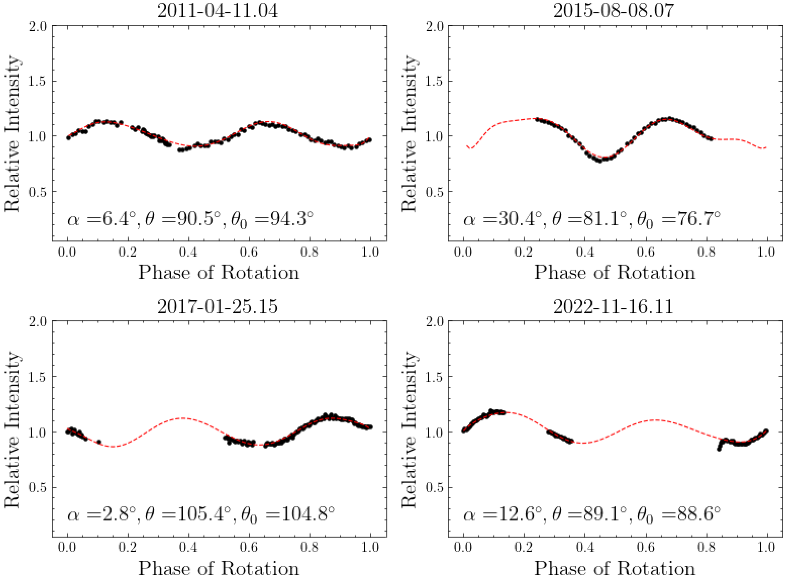
3.1. Rotation Period Analysis

To derive the rotation periods, we corrected the light travel time for each data point and fitted the light curves using a second-order Fourier serie: [22].

$$M_{i,j}=\sum _{k=1,2}^{N_k}\left\{B_{k}sin\left[{\displaystyle \frac{2\pi k}{P}}\left(t_j-t_0\right)\right]+C_{k}cos\left[{\displaystyle \frac{2\pi k}{P}}\left(t_j-t_0\right)\right]\right\}+Z_i$$

(1)

where $M_{i,j}$ is the magnitude measured at epoch $t_j$ in the corresponding band (R, I, or V), $B_k$ and $C_k$ are the Fourier coefficients, P is the rotation period, $t_0$ is an arbitrary epoch, and $Z_i$ is the offset for measurements taken on different nights. As an example, in Figure 1 we present the results of the rotation period fitting for (2253) Espinette using a second-order Fourier series method. The rotation period of (2253) Espinette was accurately determined using only the 2021 light curve data, which were sufficient for precise period determination, negating the need for additional data. This result is consistent with previous studies [23]. Additional light curve data and second-order Fourier fit plots for determining rotation periods of other asteroids can also be found in the CNEOST database.

When observational data are insufficient to cover a complete light curve or when noise levels are significant, determining the period using a second-order Fourier series presents challenges. In addition, long gaps between individual light curves can create ambiguity in the cycle count, leading to the potential for aliasing. To address these issues, we selected 892 asteroids from the CNEOST photometric survey conducted between 2015 and 2018. Each asteroid was subjected to continuous time series photometric observations over 2 to 5 days, ensuring that at least half of the light curve period was covered. We remain cautious about these results, and have examined the fitting of each asteroid individually. This careful approach allows us to derive more robust conclusions regarding the periodic behavior of these asteroids and minimizes the risk of misidentifying periods due to aliasing or insufficient data coverage.

Finally, the rotation periods of these 892 asteroids (including five NEAs) were obtained, visually reviewed, and analyzed. Unfortunately, no candidates for super-fast rotators (SFRs) were identified within our samples. To validate our analysis of the rotation periods, we compared our results with the Light Curve Database (LCDB)8 by Warner et al. [24], updated as of 1 October 2023, which archives rotation periods derived from independent light curves. The reliability of these periods in the LCDB is indicated by an uncertainty code U, where higher values signify greater reliability. For comparison, we selected asteroids with uncertainty codes of U = 2 or higher, totaling 812 cases.

To evaluate the consistency between the asteroid rotation periods obtained from the CNEOST and those listed in the LCDB, we used a relative error criterion. Results were considered consistent and reasonable if the relative error between the fitted period and the LCDB period was within 10% [25]. Of the 648 asteroids in our sample, approximately 73% had rotation periods consistent with those provided by the LCDB; specifically, 81% of asteroids marked with an uncertainty code of U = 3 in the LCDB had consistent rotation periods, compared to 79% for those with U = 2 or higher, indicating no significant differences. Figure 2 shows the diameters versus the rotation frequencies for the 892 asteroids, along with a comparison of rotation periods from both databases. For asteroids with U < 2, the rotation periods in our dataset are more reliable, as our observations almost entirely covered a full rotation period.

Table 2. Asteroids with U < 2 in LCDB, showing discrepancies in the rotation periods compared to CNEOST along with related parameters.

Asteroid	${\mathit{D}}_{\mathbf{eff}}$ *	H	Albedo	${\mathit{P}}_{\mathbf{LCDB}}$	${\mathit{P}}_{\mathbf{CNEOST}}$
	[km]	[mag]		[h]	[h]
(2113) Ehrdni	6.81	3.2	0.2	13.2	5.035
(2640) Hallstrom	7.16	3.09	0.2	22.9	11.17
(4334) Foo	11.3	3.24	0.07	7.42	11.04
(7147) Feijth	2.84	5.22	0.179	5.318	8.505
(11202) Teddunham	7.58	3.08	0.18	7.414	15.505
(12659) Schlegel	2.59	5.42	0.179	9.7	5.6975
(13014) Hasslacher	11.95	3.4	0.054	7.62	11.8075
(16115) 1999 XH25	12.48	3.28	0.0553	14.68	11.095
(17953) 1999 JB20	10.32	3.66	0.057	37.279	4.885
(38663) 2000 OK49	2.8	5.13	0.2	5.51	6.115
(42535) 1995 VN9	1.77	6.12	0.2	2.37	6.1375
(43321) 2000 JR52	2.85	5.09	0.2	4.75	3.7575
(44576) 1999 GJ10	5.83	4.9	0.057	0.48	5.5425
(55002) 2001 QF19	4.11	4.61	0.15	4.56	5.0625
(60381) 2000 AX180	15.62	2.76	0.057	28.96	5.885
(82333) 2001 LF7	5.59	4.99	0.057	2.303	19.3225
(85338) 1995 SX37	2.06	5.8	0.2	1.1	3.5825
(90050) 2002 VQ23	2.85	5.84	0.1	17.3	5.6375
(103541) 2000 BU18	4.48	5.47	0.057	7.11	6.035
(282631) 2005 SV1	2.76	5.63	0.13	16.8	6.41

* The equivalent diameter $D_{\mathrm{eff}}$ of the asteroid is calculated using the formula: $D_{\mathrm{eff}}={10}^{(3.1236-0.5lo{g}_{10}\left(p_v\right)-0.2H)}$ [26].

provides the rotation periods $P_{\mathrm{CNEOST}}$ for each asteroid derived from the CNEOST data along with the corresponding period $P_{\mathrm{LCDB}}$ reported in the LCDB by Warner et al. [24].

To expand the sample of asteroids with reliable spin parameters and shape models, we screened 648 asteroids with U = 3 and U = 2. We examined the data from which DAMIT models were derived, focusing on asteroids that lacked reliable spin parameters and shape models but had at least ten light curves from different viewing geometries and apparitions. The asteroids selected for further analysis included (2233) Kuznetsov, (2294) Andronikov, (2253) Espinette, (4796) Lewis, (1563) Noel, (2912) Lapalma, and (5150) Fellini.

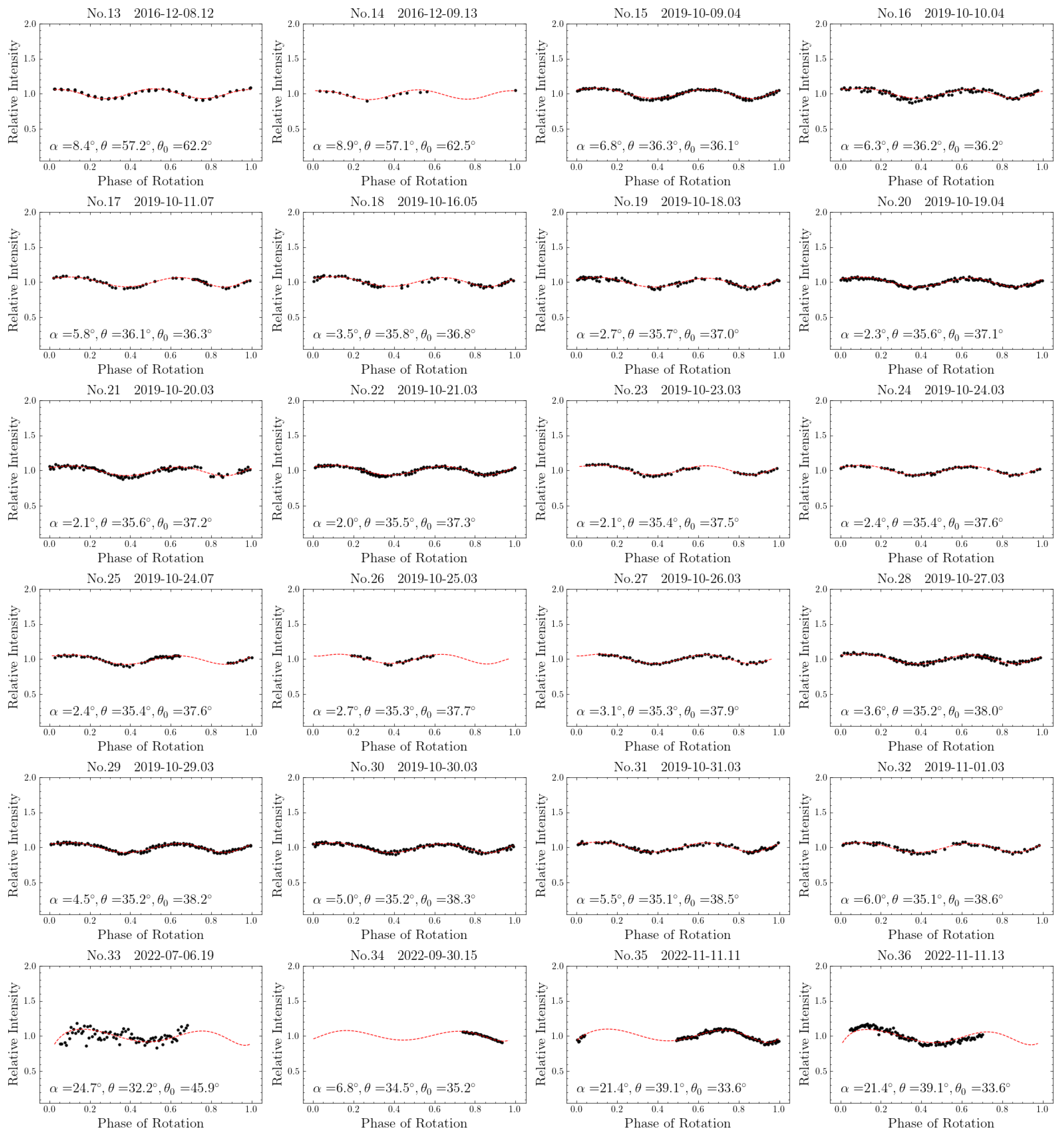
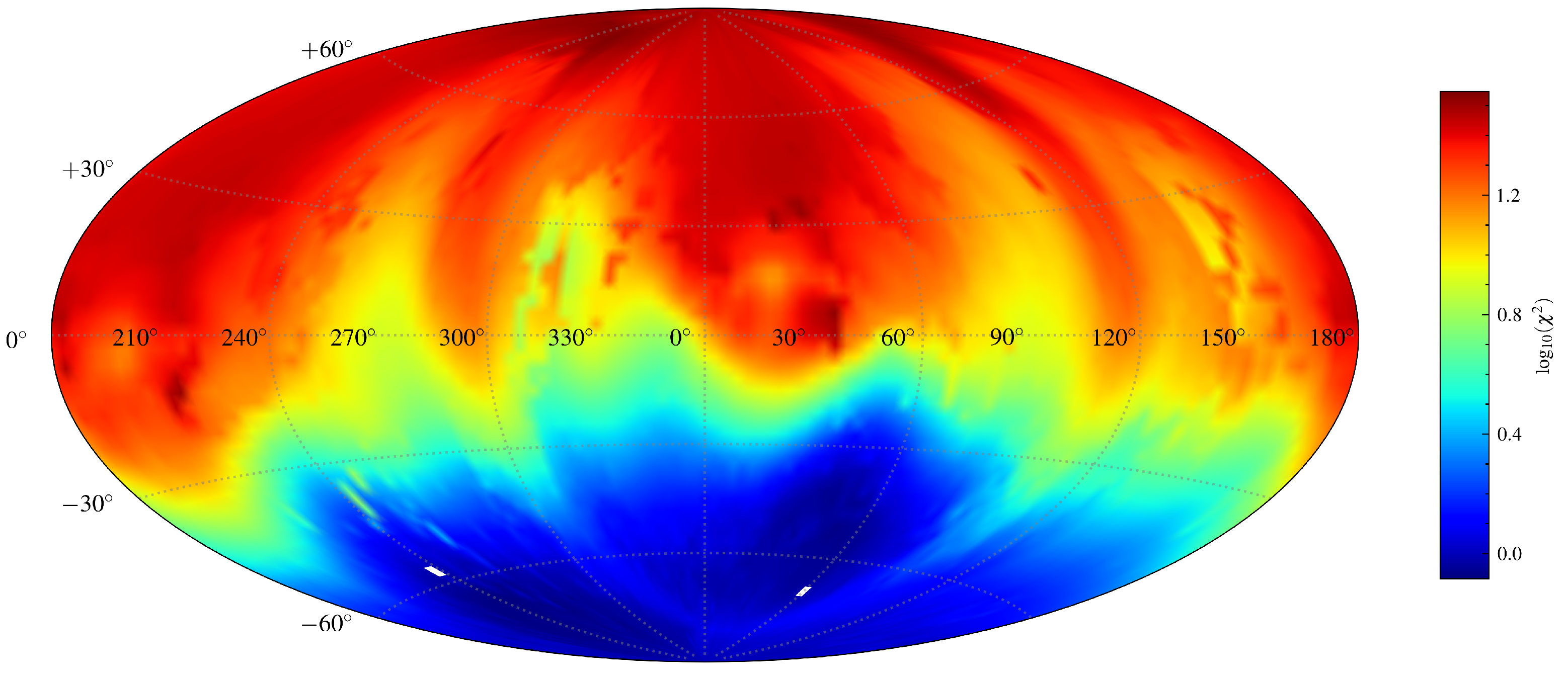
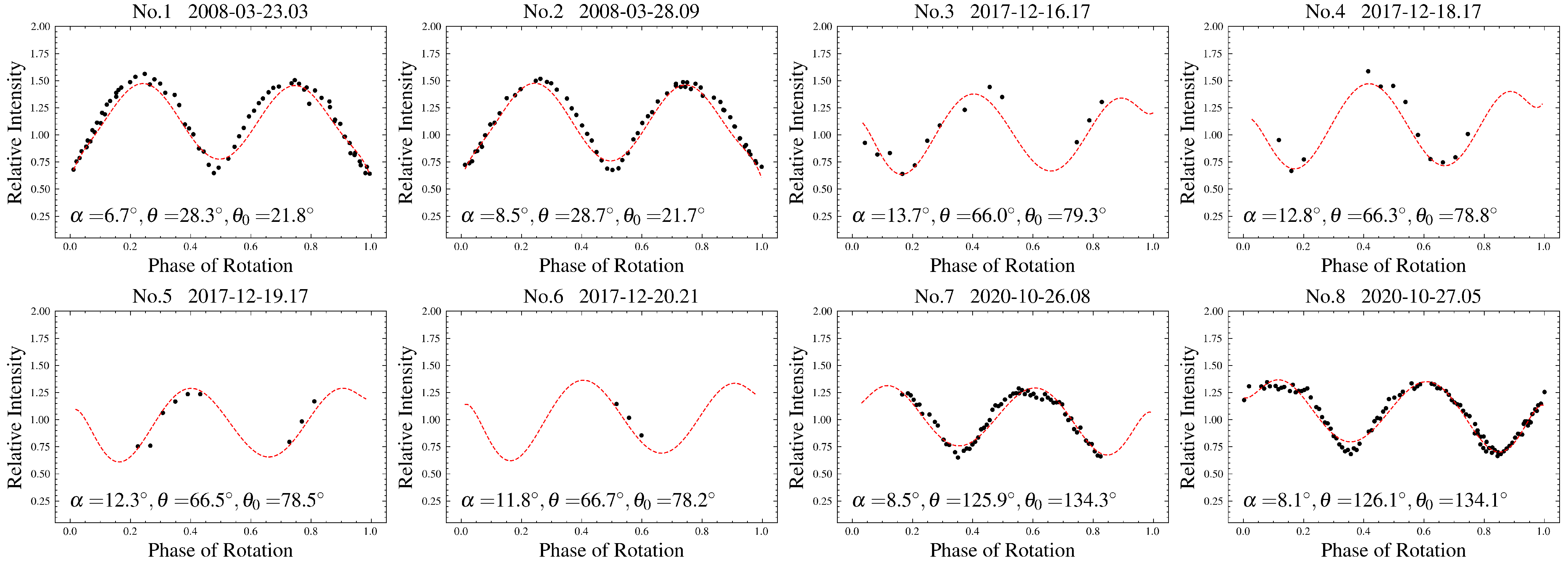
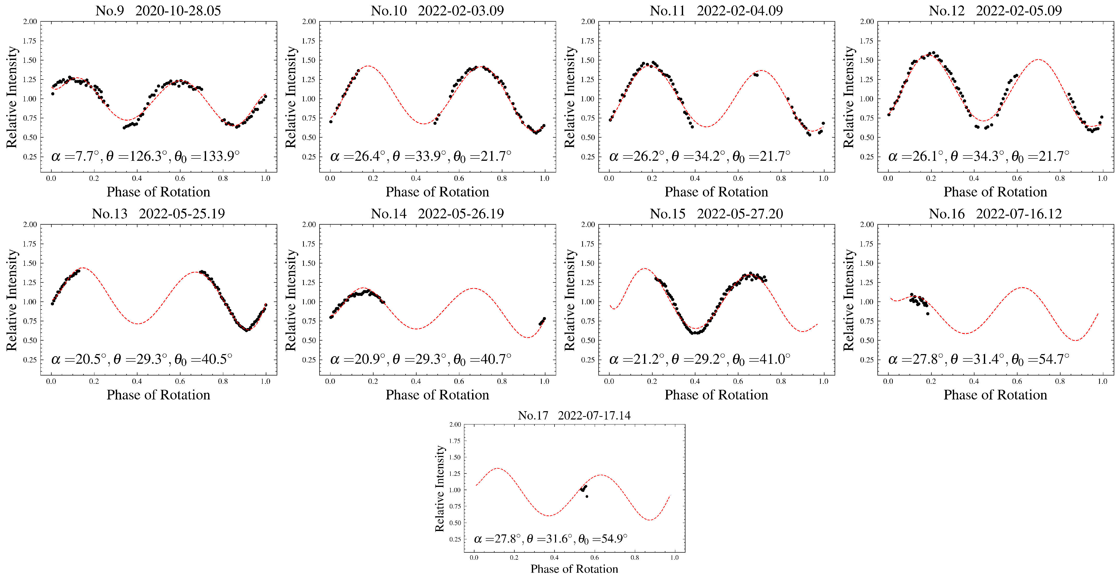
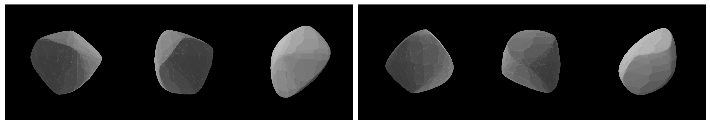
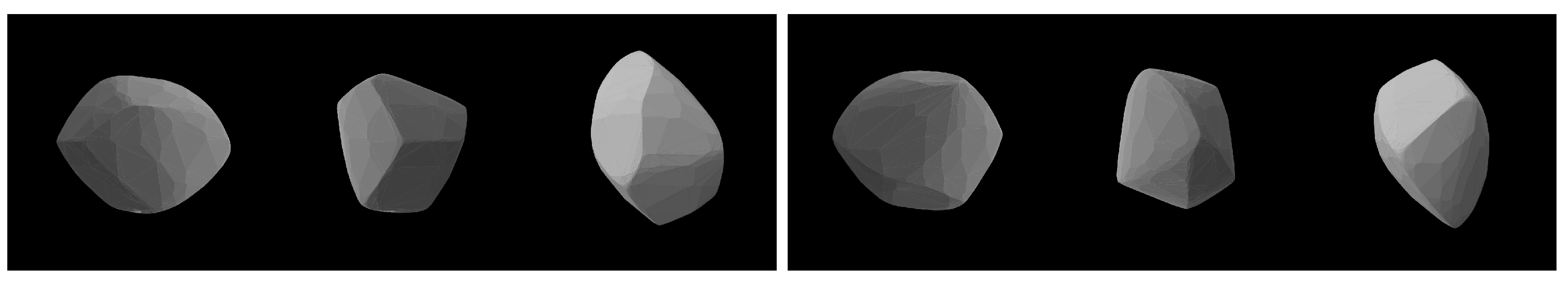
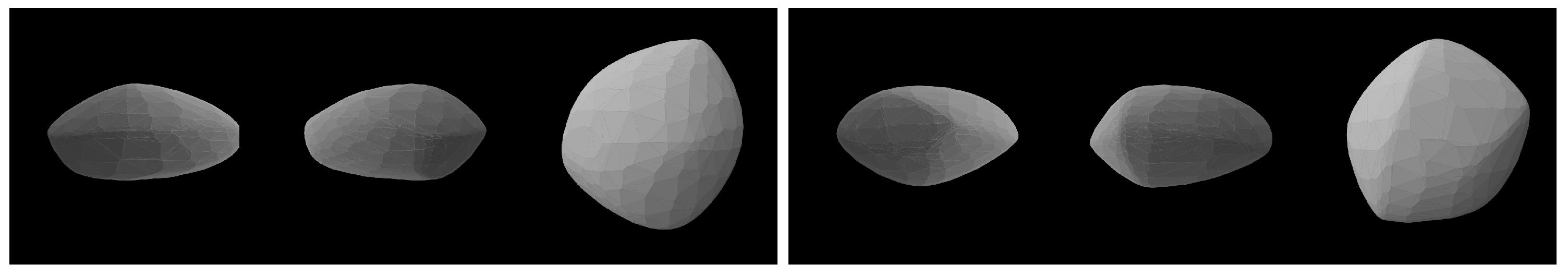
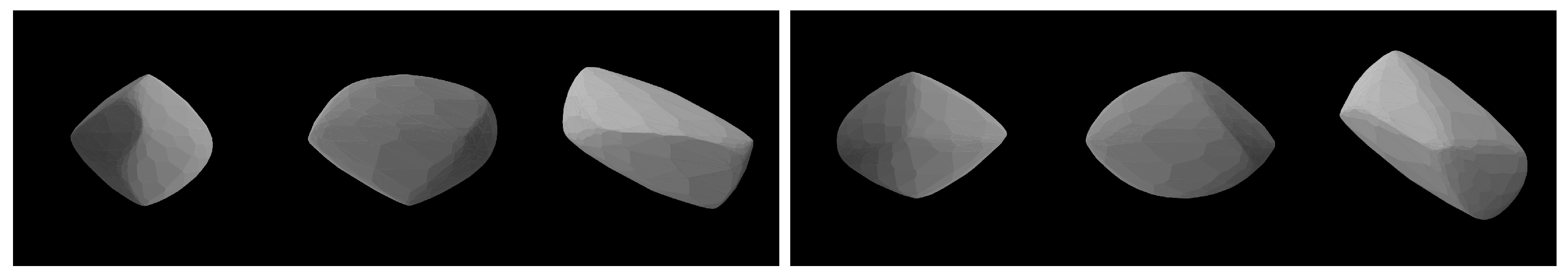
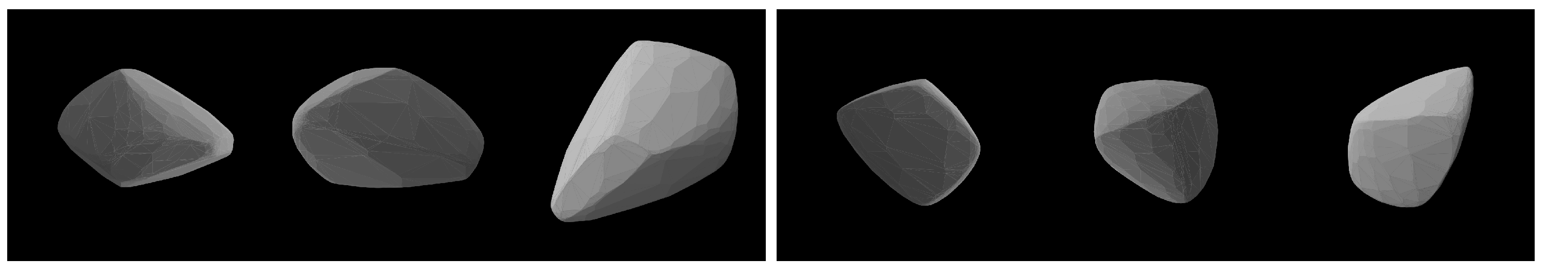
3.2. Shape and Spin Reconstruction with Light Curve Inversion

We used the standard convex inversion method [7,8] based on the inversion of photometric measurements. The convex inversion method assumes that the reflectance of the asteroid surface is provided by a combination of the Lambert and Lommel–Seeliger scattering laws:

$$S\left(\mu ,{\mu }_0,\alpha \right)=f\left(\alpha \right)\left({\displaystyle \frac{\mu {\mu }_0}{\mu +{\mu }_0}}+c\mu {\mu }_0\right)$$

(2)

where $\alpha$ is the solar phase angle (Sun–object–observer angle), $f\left(\alpha \right)$ is the phase function, $c=0.1$ is the weight factor for the Lambert term, ${\mu }_0=cosi$, $\mu =cose$ (with i and e being the angle of incidence and emergence of the light, respectively), and $f\left(\alpha \right)$ is the following phase function [27]:

$$f\left(\alpha \right)=A_{0}exp\left(-{\displaystyle \frac{\alpha }{D}}\right)+k\alpha +b$$

(3)

where $A_0$, k, and b are the three linear parameters: $A_0$ is the amplitude, k is the slope, and D is the angular width of the opposition. The optimal model is determined by achieving the best fit between the observed light curves and those calculated based on the shape model. The equation that defines this fit is provided by

$${\chi }_{rel}^2=\sum _i{∥{\displaystyle \frac{L_{obs}^{\left(i\right)}}{{\overline{L}}_{obs}^{\left(i\right)}}}-{\displaystyle \frac{L^{\left(i\right)}}{{\overline{L}}^{\left(i\right)}}}∥}^2,$$

(4)

where $L_{obs}^{\left(i\right)}$ and $L^{\left(i\right)}$ are the observed and modeled light curves, respectively, while ${\overline{L}}_{obs}^{\left(i\right)}$ and ${\overline{L}}^{\left(i\right)}$ are their mean brightness values. The index i refers to each individual sequence of light curves separately. The Levenberg–Marquardt algorithm (L-M algorithm) is used to solve the minimization problem within the convex light curve inversion method [6,8]. However, due to the localized optimization nature of the L-M algorithm, extensive scanning of spaces with large rotation period parameters is required, which necessitates additional iterations to ensure the accuracy of the inversion results.

To determine the synodic period of the asteroid, we use a second-order Fourier series for fitting, which provides an accurate approximation of the true sidereal period. This estimated period was used as a constraint on the parameter space, thereby improving computational efficiency. Subsequently, we conducted a period search employing a convex shape model, parameterized by spherical harmonics of order and degree six. The periodograms were scanned over an interval of one hour centered on the estimated period to identify an optimal rotation period, which was then used as the initial sidereal period.

Next, we searched for optimal initial values for the polar coordinates by evaluating a sky grid with a resolution of $3^{\circ }\times 3^{\circ }$. The sidereal period and convex shape were iteratively optimized to best match the observed light curves for each fixed pole position, while the initial epoch $T_0$ and rotation phase ${\varphi }_0$ remained constant. The results from the pole search for asteroid (2253) Espinette are presented in Figure 3.

Finally, the shape model was further optimized based on the initial values of the three spin parameters (P, $\lambda$, $\beta$). A globally unique solution was defined as having the lowest ${\chi }_{min}^2$, with all other solutions providing ${\chi }^2$ higher than ${\chi }_{tr}^2=(1+\sqrt{2/\nu }){\chi }_{min}^2$, where $\nu$ is the number of degrees of freedom and the root mean square (RMS) residuals of all local minima must be higher than 0.01.

The Monte Carlo method was used to estimate the errors in the spin parameters for the seven studied MBAs. This involved generating 8000 virtual light curve datasets, each with randomly added noise within their respective photometric error ranges. Specifically, we introduced normally distributed random noise at each observation point based on the photometric error. The standard deviation of this noise is associated with the corresponding photometric error. By randomly adding noise to the photometry at each observation point across the entire light curve dataset, we generated a virtual light curve dataset. This approach can simulate the photometric errors that may occur in actual observations, thereby producing a virtual dataset that accurately reflects realistic conditions. For cases where the light curves lack photometric error information, such as for asteroid (1563) Noel, for which this information was extrapolated from the MPBu [18], a Fourier series of the highest order as determined by an F-test was used to realistically estimate errors in the light curve fitting [28], as follows:

$$F_n={\displaystyle \frac{\left({\chi }_0^2-{\chi }_n^2\right)/\left({\nu }_0-{\nu }_n\right)}{{\chi }_n^2/{\nu }_n}}$$

(5)

where ${\chi }_n^2$ is the chi-square value for fitting a Fourier series of order n with ${\nu }_n=N-(2n+1)$ degrees of freedom (where N is the number of photometric points per light curve) and ${\chi }_0^2$ is the chi-square value for the light curve with ${\nu }_0=N$ degrees of freedom. The residual of the root mean square is used as the estimate for the photometric error.

Each dataset is then inverted to derive the spin parameters. The distribution of these parameters is fitted using a normal distribution to estimate the standard deviation. However, the standard deviations of these spin parameters only reflect the influence of the photometric errors in the existing light curve data.

4. Results

In total, we obtained seven unique asteroid models that passed our reliability tests. The convex inversion method can only infer coarse global-scale shape properties and fails to accurately represent the concave structures of an asteroid’s surface. These concave features typically appear as larger flat areas within the convex shape model. Nevertheless, reasonable inferences regarding the asteroid’s structural characteristics along with physical processes such as collisions and rotational fission can still be derived from the convex shape model. Furthermore, the reliability of this model is highly dependent on the quality of the photometric data used during the inversion process. Significant data errors or a lack of photometric observations across different viewing geometries can adversely impact the accuracy of the results.

We also employed the Cellinoid model [29] to validate our inversion results. The Cellinoid model provided optimal solutions for the six semi-axes (a1, a2, b1, b2, c1, c2) of these seven asteroids, enabling us to estimate their axis ratios, which we present for the first time in

Table 3. Summary of inversion results for the seven studied main belt asteroids.

Asteroid	${\mathit{P}}_{\mathbf{sid}}$	$\mathit{\lambda },\mathit{\beta }$	Axial Ratio	Obliquity *	${\mathit{D}}_{\mathbf{eff}}$
	[h]	[deg], [deg]		[deg]	[km]
(2233) Kuznetsov	$5.030425\left(3\right)$	$({147}^{\circ }\pm 1^{\circ },-{68}^{\circ }\pm 2^{\circ })$	a/c = 1.4, b/c = 1.2	154.6	6.70
	$5.030425\left(9\right)$	$({330}^{\circ }\pm 4^{\circ },-{59}^{\circ }\pm 5^{\circ })$		152.4
(2294) Andronikov	$3.002242\left(3\right)$	$({313}^{\circ }\pm 3^{\circ },-{50}^{\circ }\pm 3^{\circ })$	a/c = 2.0, b/c = 1.4	55.1	15.1
	$3.002243\left(1\right)$	$({113}^{\circ }\pm 1^{\circ },-{54}^{\circ }\pm 2^{\circ })$		50.5
(2253) Espinette	$7.443344\left(6\right)$	$({144}^{\circ }\pm 1^{\circ },-{34}^{\circ }\pm 1^{\circ })$	a/c = 1.2, b/c = 1.0	123.9	6.23
	$7.443345\left(7\right)$	$({322}^{\circ }\pm 2^{\circ },-{35}^{\circ }\pm 2^{\circ })$		125.0
(4796) Lewis	$3.508346\left(1\right)$	$({73}^{\circ }\pm 3^{\circ },{35}^{\circ }\pm 3^{\circ })$	a/c = 1.9, b/c = 1.1	56.6	4.20
	$3.508346\left(1\right)$	$({253}^{\circ }\pm 3^{\circ },{27}^{\circ }\pm 3^{\circ })$		61.5
(1563) Noel	$3.548785\left(1\right)$	$({117}^{\circ }\pm 4^{\circ },-{54}^{\circ }\pm 2^{\circ })$	a/c = 2.5, b/c = 2.2	149.3	7.24
	$3.548784\left(3\right)$	$({292}^{\circ }\pm 4^{\circ },-{68}^{\circ }\pm 2^{\circ })$		152.7
(2912) Lapalma	$5.710868\left(2\right)$	$({60}^{\circ }\pm 2^{\circ },-{67}^{\circ }\pm 2^{\circ })$	a/c = 2.0, b/c = 1.0	151.2	6.52
	$5.710865\left(2\right)$	$({231}^{\circ }\pm 6^{\circ },-{56}^{\circ }\pm 5^{\circ })$		151.9
(5150) Fellini	$5.195770\left(28\right)$	$({302}^{\circ }\pm {10}^{\circ },-{48}^{\circ }\pm {21}^{\circ })$	a/c = 2.2, b/c = 1.0	131.3	5.40
	$5.195763\left(4\right)$	$({115}^{\circ }\pm 3^{\circ },-{38}^{\circ }\pm 2^{\circ })$		134.6

* The obliquity, which is the angle between the rotational pole of the asteroid and its orbital momentum, is calculated using the proper orbital inclination and longitude of the ascending node obtained through the Horizons ephemeris system from JPL (https://ssd.jpl.nasa.gov, accessed on 21 July 2024).

. For all cases, we identified two possible pole solutions, each with nearly identical pole latitudes $\beta$ and pole longitudes $\lambda$ differing by approximately ${180}^{\circ }$. This ambiguity arises from the symmetry of the problem, as observations confined to the ecliptic plane inherently lead to this $\lambda \pm {180}^{\circ }$ ambiguity [30]. Consequently, deriving spin parameters and shape models for MBAs may necessitate longer durations of photometric data collection across various viewing geometries.

The shape model obtained from the convex light curve inversion method is not scaled to size, resulting in arbitrary units for the x, y, and z axes. In this model, the z-axis aligns with the shortest axis of inertia, which also corresponds to the spin axis. The shape model views are presented along the x, y, and z axes. Figure 4, Figure 5, Figure 6, Figure 7, Figure 8, Figure 9 and Figure 10 show the shape models of seven asteroids, showing no significant differences between the two solutions for each asteroid. The sample light curve fits are plotted in relative intensity, with the mean intensity of the observed points normalized to one. This format is preferred because it corresponds directly to the physical observable (photon count) of the object, providing a well defined zero line. The modeling procedure fits the intensity rather than the magnitude, as intensity is a more direct measurement. For each asteroid, we provide two shape solutions that match the synthetic light curves with the observed data. These solutions are listed in Table 3 ranked by fit quality, with the first solution selected for presentation in the fitting results of the following subsection. As an example, the fitting results for (2253) Espinette are shown in Figure 11. The light curve fitting results for all seven asteroids are provided in Appendix A.

Asteroid (2233) Kuznetsov exhibits an oblate spheroidal shape, with approximate dimension ratios of a/c = 1.4 and b/c = 1.2. Although its light curves are generally smooth and regular, some irregularities are present in its shape. In contrast, (2253) Espinette is nearly spherical, with dimension ratios of a/c = 1.2 and b/c = 1.0. Neither of these asteroids shows significant large-scale planar structures. The analysis utilizes a substantial number of light curves which provide good coverage of the geometries. The synthetic light curves generated by the models fit well with the observed data, indicating that reliable shape solutions were obtained.

Asteroid (2294) Andronikov has an axis ratio of approximately a/c = 2.0 and b/c = 1.4, indicating a significantly elongated shape. Similarly, (4796) Lewis displays a large planar dimension, likely resulting from fitting a light curve with a larger amplitude. This observation implies that the current light curve constraints are insufficient and that the flexibility in adjusting various geometric structures to fit the light curves decreases as the dataset expands. The light curve fit for (2294) Andronikov in 2016 was notably poor, while the other fits were satisfactory, indicating that the shape models for these two asteroids may still be preliminary.

Asteroid (1563) Noel has a notably flattened shape, with axis ratios of approximately a/c = 2.5 and b/c = 2.2. The shape model is derived from 36 light curves across five apparitions, offering good coverage of the solar phase angle. This morphology features an equatorial bulge, identifying the asteroid as a “top-shaped” object. This is likely a result of surface reformation due to rapid rotation, which is consistent with its short rotation period.

Asteroids (2912) Lapalma and (5150) Fellini both exhibit highly elongated shapes. (2912) Lapalma likely has a cylindrical structure, with large-scale planar features that might correspond to depressions; its barrel-like shape could even suggest a contact binary structure with a possible concave ‘waist’. In contrast, (5150) Fellini has a cone-like and highly irregular shape. The light curves for both shape solutions of these asteroids do not show significant differences. However, the fits for the two light curves from 2015 were notably poor and the parameters for the second shape solution exhibited large errors, indicating that these models remain preliminary.

Based on the shape models presented above, the future acquisition of radar, interferometry, adaptive optics, and occultation data will provide strong constraints for these shape models. These data will not only facilitate the determination of physical parameters such as the size, roughness, and composition of these asteroids, but also allow for further inferences regarding their possible evolutionary processes.

5. Conclusions

We initially analyzed photometric data obtained by CNEOST from four photometric surveys conducted between 2015 to 2018, deriving the rotation periods of 892 asteroids using a second-order Fourier series. The results show that approximately 73% of these asteroids have rotation periods consistent with those listed in the LCDB. By expanding the sample of asteroids with reliable rotation periods, our results enhance the statistical significance in studying the evolution of rotation periods influenced by asteroid collisions and non-gravitational effects, in particular the Yarkovsky–O’Keefe–Radzievskii–Paddack (YORP) effect. Additionally, we present the first measurements of the spin parameters and shapes of seven MBAs using independent photometric data through the convex light curve inversion method. This expands the current dataset of asteroids with inferred spin parameters and shapes, thereby supporting future research on asteroid rotation dynamics and shape distribution. Ultimately, these results contribute to a more comprehensive understanding of the formation and evolution of asteroids.

In addition, comparison with DAMIT will support future updates to the spin parameters and shape models of 188 asteroids, particularly those derived entirely from sparse photometric data. This paper presents an analysis of data from the ongoing CNEOST photometric survey of asteroids, which offers opportunities for future inversion to refine models and specifically investigate the YORP effect in NEAs. Furthermore, our future work will place greater emphasis on comparing these asteroids with the general population, which could enhance our understanding of their formation and evolution.

References

1. Davis, D.R.; Weidenschilling, S.J.; Farinella, P.; Paolicchi, P.; Binzel, R.P. Asteroid collisional history: Effects on sizes and spins. In Asteroids II; Binzel, R.P., Gehrels, T., Matthews, M.S., Eds.; University of Arizona Press: Tucson, AZ, USA, 1989; pp. 805–826. [Google Scholar]
2. Rossi, A.; Marzari, F.; Scheeres, D.J.; Jacobson, S. Effects of YORP-Induced Rotational Fission on the Asteroid Size Distribution at the Small Size End. In Proceedings of the 43rd Annual Lunar and Planetary Science Conference, The Woodlands, TX, USA, 19–23 March 2012; p. 2095. [Google Scholar]
3. Scheeres, D.J.; Fahnestock, E.G.; Ostro, S.J.; Margot, J.L.; Benner, L.A.M.; Broschart, S.B.; Bellerose, J.; Giorgini, J.D.; Nolan, M.C.; Magri, C.; et al. Dynamical Configuration of Binary Near-Earth Asteroid (66391) 1999 KW4. Science 2006, 314, 1280–1283. [Google Scholar] [CrossRef] [PubMed]
4. Nolan, M.C.; Magri, C.; Howell, E.S.; Benner, L.A.M.; Giorgini, J.D.; Hergenrother, C.W.; Hudson, R.S.; Lauretta, D.S.; Margot, J.L.; Ostro, S.J.; et al. Shape model and surface properties of the OSIRIS-REx target Asteroid (101955) Bennu from radar and lightcurve observations. Icarus 2013, 226, 629–640. [Google Scholar] [CrossRef]
5. Li, X.; Scheeres, D.J. The shape and surface environment of 2016 HO3. Icarus 2021, 357, 114249. [Google Scholar] [CrossRef]
6. Ďurech, J.; Sidorin, V.; Kaasalainen, M. DAMIT: A database of asteroid models. Astron. Astrophys. 2010, 513, A46. [Google Scholar] [CrossRef]
7. Kaasalainen, M.; Torppa, J. Optimization Methods for Asteroid Lightcurve Inversion: I. Shape Determination. Icarus 2001, 153, 24–36. [Google Scholar] [CrossRef]
8. Kaasalainen, M.; Torppa, J.; Muinonen, K. Optimization Methods for Asteroid Lightcurve Inversion: II. The Complete Inverse Problem. Icarus 2001, 153, 37–51. [Google Scholar] [CrossRef]
9. Kaasalainen, M.; Ďurech, J. Asteroid models from generalised projections: Essential facts for asteroid modellers and geometric inverse problem solvers. arXiv 2020, arXiv:2005.09947. [Google Scholar]
10. Zhaori, G.T.; Zhao, H.B.; Liu, W.; Li, B. Correction of Off-axis Aberration of the China Near Earth Object Survey Telescope with 10k CCD. Acta Astron. Sin. 2019, 60, 52. [Google Scholar]
11. Molotov, I.; Agapov, V.; Kouprianov, V.; Titenko, V.; Rumyantsev, V.; Biryukov, V.; Borisov, G.; Burtsev, Y.; Khutorovsky, Z.; Kornienko, G.; et al. ISON Worldwide Scientific Optical Network. In Proceedings of the Fifth European Conference on Space Debris, Darmstadt, Germany, 30 March–2 April 2009; Lacoste, H., Ed.; ESA Special Publication: Noordwijk, The Netherlands, 2009; Volume 672, p. 7. [Google Scholar]
12. Tody, D. The IRAF Data Reduction and Analysis System. In Proceedings of the Instrumentation in Astronomy VI, Tucson, AZ, USA, 1–2 March 1986; Crawford, D.L., Ed.; Society of Photo-Optical Instrumentation Engineers (SPIE) Conference Series. SPIE: St. Bellingham, WA, USA, 1986; Volume 627, p. 733. [Google Scholar] [CrossRef]
13. Tody, D. IRAF in the Nineties. In Astronomical Data Analysis Software and Systems II; Hanisch, R.J., Brissenden, R.J.V., Barnes, J., Eds.; Astronomical Society of the Pacific Conference Series; Astronomical Society of the Pacific: San Francisco, CA, USA, 1993; Volume 52, p. 173. [Google Scholar]
14. Gaia Collaboration; Vallenari, A.; Brown, A.G.A.; Prusti, T.; de Bruijne, J.H.J.; Arenou, F.; Babusiaux, C.; Biermann, M.; Creevey, O.L.; Ducourant, C.; et al. Gaia Data Release 3. Summary of the content and survey properties. Astron. Astrophys. 2023, 674, A1. [Google Scholar] [CrossRef]
15. Zacharias, N.; Finch, C.T.; Girard, T.M.; Henden, A.; Bartlett, J.L.; Monet, D.G.; Zacharias, M.I. The Fourth US Naval Observatory CCD Astrograph Catalog (UCAC4). Astron. J. 2013, 145, 44. [Google Scholar] [CrossRef]
16. Howell, S.B. Handbook of CCD Astronomy; Cambridge University Press: Cambridge, UK, 2000. [Google Scholar]
17. Demleitner, M.; Accomazzi, A.; Eichhorn, G.; Grant, C.S.; Kurtz, M.J.; Murray, S.S. ADS’s Dexter Data Extraction Applet. In Proceedings of the Astronomical Data Analysis Software and Systems X, Boston, MA, USA, 12–15 November 2000; Harnden, F.R.J., Primini, F.A., Payne, H.E., Eds.; Astronomical Society of the Pacific Conference Series. Astronomical Society of the Pacific: San Francisco, CA, USA, 2001; Volume 238, p. 321. [Google Scholar]
18. Apostolovska, G.; Kostov, A.; Donchev, Z.; Ovcharov, E. Lightcurve of 1563 Noel at Low Phase Angle. Minor Planet Bull. 2017, 44, 143. [Google Scholar]
19. Brinsfield, J.W. Asteroid Lightcurve Analysis at the via Capote Observatory: First Quarter 2008. Minor Planet Bull. 2008, 35, 119–122. [Google Scholar]
20. Carbognani, A. Lightcurve and Rotational Period of Asteroids 1456 Saldanha, 2294 Andronikov, and 2006 NM. Minor Planet Bull. 2007, 34, 4–5. [Google Scholar]
21. Carbo, L.; Green, D.; Kragh, K.; Krotz, J.; Meiers, A.; Patino, B.; Pligge, Z.; Shaffer, N.; Ditteon, R. Asteroid Lightcurve Analysis at the Oakley Southern Sky Observatory: 2008 October thru 2009 March. Minor Planet Bull. 2009, 36, 152–157. [Google Scholar]
22. Harris, A.W.; Young, J.W.; Bowell, E.; Martin, L.J.; Millis, R.L.; Poutanen, M.; Scaltriti, e.a. Photoelectric observations of asteroids 3, 24, 60, 261, and 863. Icarus 1989, 77, 171–186. [Google Scholar] [CrossRef]
23. Warner, B.D.; Harris, A.W.; Pravec, P.; Durech, J.; Benner, L.A.M. Lightcurve Photometry Opportunities: July–September 2008. Minor Planet Bull. 2008, 35, 139–141. [Google Scholar]
24. Warner, B.D.; Harris, A.W.; Pravec, P. The asteroid lightcurve database. Icarus 2009, 202, 134–146. [Google Scholar] [CrossRef]
25. Ďurech, J.; Hanuš, J. Reconstruction of asteroid spin states from Gaia DR3 photometry. Astron. Astrophys. 2023, 675, A24. [Google Scholar] [CrossRef]
26. Fowler, J.W.; Chillemi, J.R. IRAS Minor Planet Survey; Phillips Laboratory Technical Report No. PL-TR-92-2049; Phillips Laboratory, Directorate of Geophysics, Air Force Materiel Command: Hanscom Air Force Base, MA, USA, 1992. [Google Scholar]
27. Muinonen, K.; Penttilä, A.; Cellino, A.; Belskaya, I.N.; Delbò, M.; Levasseur-Regourd, A.C.; Tedesco, E.F. Asteroid photometric and polarimetric phase curves: Joint linear-exponential modeling. Meteorit. Planet. Sci. 2009, 44, 1937–1946. [Google Scholar] [CrossRef]
28. Magnusson, P.; Dahlgren, M.; Barucci, M.A.; Jorda, L.; Binzel, R.P.; Slivan, S.M.; Blanco, C.; Riccioli, D.; Buratti, B.J.; Colas, F.; et al. Photometric Observations and Modeling of Asteroid 1620 Geographos. Icarus 1996, 123, 227–244. [Google Scholar] [CrossRef]
29. Lu, X.; Zhao, H.; You, Z. Cellinoid Shape Model for Asteroids. Earth Moon Planets 2014, 112, 73–87. [Google Scholar] [CrossRef]
30. Kaasalainen, M.; Lamberg, L. Inverse problems of generalized projection operators. Inverse Probl. 2006, 22, 749–769. [Google Scholar] [CrossRef]
31. Stephens, R.D. Asteroids Observed from CS3: 2016–September. Minor Planet Bull. 2017, 44, 49–52. [Google Scholar] [PubMed]
32. Skiff, B.A.; McLelland, K.P.; Sanborn, J.J.; Pravec, P.; Koehn, B.W. Lowell Observatory Near-Earth Asteroid Photometric Survey (NEAPS): Paper 3. Minor Planet Bull. 2019, 46, 238–265. [Google Scholar]
33. Stephens, R.D. Asteroids Observed from CS3: 2015 July–September. Minor Planet Bulletin 2016, 43, 52–56. [Google Scholar]
34. Stephens, R.D.; Coley, D.R.; Warner, B.D. Main-belt Asteroids Observed from CS3: 2021 January to March. Minor Planet Bull. 2021, 48, 246–267. [Google Scholar]
35. Hasegawa, S.; Miyasaka, S.; Mito, H.; Sarugaku, Y.; Ozawa, T.; Kuroda, D.; Nishihara, S.; Harada, A.; Yoshida, M.; Yanagisawa, K.; et al. Lightcurve survey of V-type asteroids in the inner asteroid belt. Publ. Astron. Soc. Jpn. 2014, 66, 54. [Google Scholar] [CrossRef]
36. Oszkiewicz, D.A.; Skiff, B.A.; Moskovitz, N.; Kankiewicz, P.; Marciniak, A.; Licandro, J.; Galiazzo, M.A.; Zeilinger, W.W. Non-Vestoid candidate asteroids in the inner main belt. Astron. Astrophys. 2017, 599, A107. [Google Scholar] [CrossRef]
37. Polishook, D. Lightcurves and Spin Periods from the Wise Observatory: 2008 August–2009 March. Minor Planet Bull. 2009, 36, 104–107. [Google Scholar]
38. Erasmus, N.; McNeill, A.; Mommert, M.; Trilling, D.E.; Sickafoose, A.A.; van Gend, C. Taxonomy and Light-curve Data of 1000 Serendipitously Observed Main-belt Asteroids. Astrophys. J. Suppl. Ser. 2018, 237, 19. [Google Scholar] [CrossRef]
39. Oey, J. Lightcurve Analysis of Asteroids from Leura and Kingsgrove Observatories in the First Half of 2008. Minor Planet Bull. 2009, 36, 4–6. [Google Scholar]
40. Stephens, R.D.; Warner, B.D. Main-Belt Asteroids Observed from CS3: 2019 October to December. Minor Planet Bull. 2020, 47, 125–133. [Google Scholar]
41. Stephens, R.D.; Warner, B.D. Main-belt Asteroids Observed from CS3: 2020 October to December. Minor Planet Bull. 2021, 48, 150–158. [Google Scholar]
Figure 1. The left panel shows the χ 2 distribution of rotation periods fitted using a second-order Fourier series, with the minimum χ 2 corresponding to a rotation period of P = 7.4249 h. The right panel shows folded light curves of (2253) Espinette from a single apparition, with an epoch of J D 0 = 2,459,295.649215. Different markers represent photometric data collected on various observing nights (refer to Table A2). The x-axis represents the rotation phase, while the y-axis shows the apparent magnitude.
Universe 10 00395 g001
Figure 2. The left panel displays a plot of asteroid diameters versus rotation frequency, with the red, blue, and black dots respectively representing asteroids with U = 3, U = 2, and other uncertainty codes in our samples. The right panel provides a comparative illustration of the rotation periods for the same set of asteroids, as recorded in both the LCDB and CNEOST; the red shaded area highlights where the relative error between the rotation periods reported by CNEOST and LCDB is within 10%.
Universe 10 00395 g002
Figure 3. The χ 2 values for all spin axis solutions plotted on a longitude–latitude plane using an Aitoff projection of the sky in ecliptic coordinates. The plot reveals two local minima for the pole position, with the minimum χ 2 value highlighted in white for better visibility. These minima correspond to the initial spin pole values of ( λ , β ) = ( 138 , 33 ) and ( λ , β ) = ( 315 , 33 ), where λ and β represent the ecliptic longitude and latitude of the pole, respectively.
Universe 10 00395 g003
Figure 4. Convex shape models for (2233) Kuznetsov are shown from the equatorial view (y-axis on the left and x-axis at the center, 90 apart) and pole-on (z-axis on the right). The shape on the left is reconstructed from the light curves using the best-fit spin parameters ( P , λ , β ) = ( 5.030425 h , 147 , 68 ) , while the shape on the right is reconstructed using the second-best spin parameters ( P , λ , β ) = ( 5.030425 h , 330 , 59 ) .
Universe 10 00395 g004
Figure 5. As in Figure 4, the convex shape models of (2294) Andronikov are reconstructed using spin parameters ( P , λ , β ) = ( 3.002242 h , 313 , 50 ) and ( P , λ , β ) = ( 3.002243 h , 113 , 54 ) .
Universe 10 00395 g005
Figure 6. As in Figure 4, the convex shape models of (2253) Espinette are reconstructed using spin parameters ( P , λ , β ) = ( 7.443344 h , 144 , 34 ) and ( P , λ , β ) = ( 7.443345 h , 322 , 35 ) .
Universe 10 00395 g006
Figure 7. As in Figure 4, the convex shape models of (4796) Lewis are reconstructed using spin parameters ( P , λ , β ) = ( 3.508346 h , 73 , 35 ) and ( P , λ , β ) = ( 3.508346 h , 253 , 27 ) .
Universe 10 00395 g007
Figure 8. As in Figure 4, the convex shape models of (1563) Noel are reconstructed using spin parameters ( P , λ , β ) = ( 3.548785 h , 117 , 54 ) and ( P , λ , β ) = ( 3.548784 h , 292 , 68 ) .
Universe 10 00395 g008
Figure 9. As in Figure 4, the convex shape models of (2912) Lapalma are reconstructed using spin parameters ( P , λ , β ) = ( 5.710868 h , 60 , 67 ) and ( P , λ , β ) = ( 5.710865 h , 231 , 56 ) .
Universe 10 00395 g009
Figure 10. As in Figure 4, the convex shape models of (5150) Fellini are reconstructed using spin parameters ( P , λ , β ) = ( 5.195763 h , 115 , 38 ) and ( P , λ , β ) = ( 5.195770 h , 302 , 48 ) .
Universe 10 00395 g010
Figure 11. Example light curves of (2253) Espinette (black dots) alongside the synthetic light curves (red dashed curves) produced by the convex shape model with spin parameters ( P , λ , β ) = ( 7.443344 h , 144 , 34 ) .
Universe 10 00395 g011