Galaxy Classification Using EWGC

Abstract

The Enhanced Wide-field Galaxy Classification Network (EWGC) is a novel architecture designed to classify spiral and elliptical galaxies using Wide-field Infrared Survey Explorer (WISE) images. The EWGC achieves an impressive classification accuracy of 90.02%, significantly outperforming the previously developed WGC network and underscoring its superior performance in galaxy morphology classification. Remarkably, the network demonstrates a consistent accuracy of 90.02% when processing both multi-target and single-target images. Such robustness indicates the EWGC’s versatility and potential for various applications in galaxy classification tasks.

1. Introduction

The infrared band is crucial in astronomical observations, offering the ability to penetrate the dust and reveal celestial structures and phenomena that are challenging to observe in the visible band. This capability provides essential insights into the internal structure and evolutionary processes of galaxies. With the advancement of astronomical technology, the quantity and performance of infrared telescopes have significantly improved, enhancing the value of infrared astronomical research.

For instance, the launch of the Infrared Astronomical Satellite (IRAS) [1] in 1983 marked a pioneering effort in infrared surveys; the Infrared Space Observatory (ISO) [2] in 1995 enhanced observational accuracy and coverage; The Spitzer Space Telescope [3] launched in 2003, delivered high-resolution infrared images; The Wide-field Infrared Survey Explorer (WISE) [4] in 2009 covered the entire sky and amassed a vast amount of high-quality infrared data. The James Webb Space Telescope (JWST) [5], launched in December 2021, has significantly increased the depth and sensitivity of infrared observations.

In this paper, the data utilized are derived from WISE. Since its launch on 14 December 2009, WISE has systematically conducted infrared observations of the entire sky. Covering four infrared bands (W1, W2, W3, and W4, corresponding to 3.4, 4.6, 12, and 22 microns, respectively), WISE has detected hundreds of millions of stars and galaxies, thereby amassing a wealth of high-quality infrared image data.

In recent years, Convolutional Neural Networks (CNNs) and Transformer networks have made significant advancements in the field of galaxy morphology classification, presenting new opportunities and challenges. For example, Zhu et al. [6] employed the ResNet for galaxy morphology classification on the Galaxy Zoo 2 dataset, achieving an overall accuracy of 95.21%. Wu et al. [7] developed the GalSpecNet convolutional neural network model to classify emission-line galaxy spectra, attaining an accuracy of over 93% in their classification tasks. This model was also successfully applied to the SDSS DR16 and LAMOST DR8 datasets to produce a public catalog of 41,699 star-forming candidate galaxies and 55,103 AGN candidate galaxies. Wang et al. [8] applied the RepViT, which integrates the strengths of convolutional neural networks (CNNs) and visual transformers (ViTs), for a five-class galaxy morphology classification task, and achieved an accuracy of 98%. These study results demonstrate that deep learning techniques substantially enhance the accuracy of galaxy classification, laying a robust foundation for future research.

In the task of galaxy morphology classification, CNNs, and Transformer networks have been extensively researched and have achieved significant progress. Concurrently, increasingly efficient network architectures are emerging, demonstrating strong potential. Notable examples include VMamba [9], RMT [10], StarNet [11], and EfficientFormerV2 [12]. VMamba achieves the retention of a global receptive field through Visual State Space (VSS) blocks and Cross-Scan Modules (CSM) while maintaining linear computational complexity. RMT utilizes explicit decay and a Manhattan distance-based spatial decay matrix to retain the global receptive field, also achieving linear computational complexity. StarNet employs the star operation to map high-dimensional implicit feature spaces, achieving efficient image classification performance while maintaining a streamlined design. EfficientFormerV2 combines the self-attention mechanism of Transformers with the local perception capability of CNNs, optimizing network structure and lightweight design to achieve efficient image classification performance, making it an ideal choice for large-scale image classification tasks.

The objective is to enhance galaxy classification capabilities by refining the EfficientFormerV2 architecture through an innovative approach that leverages its strengths. To address this challenge, a lightweight, learnable upsampling framework, termed “Dysample”, is introduced to enhance overall classification accuracy and efficiency, particularly for small-scale targets.

The structure of this paper is organized as follows: Section 2 describes the dataset, data band fusion, and data preprocessing techniques; Section 3 provides a detailed description of the classification model and its modified version (incorporating WISE magnitude); Section 4 presents and discusses the experimental results; finally, Section 5 summarizes the main conclusions of the paper and outlines future research work.

2. Data

To acquire the necessary galaxy data from WISE, a cross-matching with the Galaxy Zoo 2 dataset [13] is utilized to ensure precise labeling of galaxy types. A crossover radius of 5 arcseconds is employed using the nearest-neighbor principle to account for pixel scale differences between SDSS (0.396 arcsec/pix) and WISE (1.375 arcsec/pix), which minimizes photometric center offsets and ensures accurate galaxy target labeling. The Galaxy Zoo 2 dataset comprises classifications from volunteers who completed 11 tasks and provided 37 responses for each galaxy image. By leveraging this dataset, a collection of 12,852 elliptical galaxies and 12,088 spiral galaxies was identified through a systematic process of visual inspection and classification.

In addition, using a cropped image size of 46.75 arcseconds (34 pixels) ensures that galaxy targets are consistently centered. The previously mentioned cross-matching radius of 5 arcseconds, combined with the WISE pixel scale of approximately 1.375 arcseconds per pixel, translates to an effective radius of about 3.6 pixels on the WISE images. This configuration allows the 34-pixel cropped image to accommodate the radius, permitting a center offset of 3.6 pixels and ensuring that the target galaxies are accurately positioned at the center. Consequently, this method enhances the reliability and accuracy of data marking. Accuracy is defined as the ratio of the number of correctly classified samples to the total number of samples. Finally, the identified galaxies are divided into training, validation, and test sets in a proportion of 7:2:1, with the detailed parameters presented in

Table 1. Galaxy parameter filtering.

Class	Task	Galaxy Zoo 2 Threshold Setting	Amount	Redshift
Spiral	T01	$f_{\mathrm{features}/\mathrm{disk}}\ge 0.430$	12,088	0–0.0736
	T02	$f_{\mathrm{edge}-\mathrm{on},\mathrm{no}}\ge 0.715$
	T04	$f_{\mathrm{spiral},\mathrm{yes}}\ge 0.619$
Elliptical	T01	$f_{\mathrm{smooth}}\ge 0.469$	12,852	0–0.0828
	T07	$f_{\mathrm{completely}\_\mathrm{round}}\ge 0.5$

Note: $f_{\mathrm{features}/\mathrm{disk}}$ is the frequency of smooth and disk-like structure, $f_{\mathrm{edge}\_\mathrm{on},\mathrm{on}}$ is the frequency of an image without lateral edges, and $f_{\mathrm{spiral},\mathrm{yes}}$ is the frequency of an image that is a spiral galaxy. Note: For T01 (“Is the galaxy simply smooth and rounded, with no sign of a disk?”), the options were as follows: smooth; features or disk; star or artifact. For T02 (“Could this galaxy have a disk or spiral arm?”), the options were as follows: edge-on disk; spiral; other. For T04 (“How many spiral arms are there?”), the options were as follows: 1 arm; 2 arms; 3 arms; 4+ arms; no spiral arms. For T07 (“Is there any sign of a merger or interaction?”), the options were as follows: yes; no.

.

The classification of spiral and elliptical galaxies in the Galaxy Zoo 2 dataset was conducted using a series of stringent threshold criteria to ensure morphological accuracy (Table 1). For spiral galaxies, the selection process first requires the frequency of disk or smooth structures (T01) to be no less than 0.430, ensuring that the chosen galaxies exhibit prominent disk structures. Additionally, the frequency of non-edge views (T02) must reach 0.715 or higher to reduce errors caused by edge-on perspectives and to enhance the clarity of spiral structures. Furthermore, the frequency of identified spiral structures (T04) must not fall below 0.619, ensuring that the galaxies possess a distinct spiral morphology. These conditions effectively filter out readily identifiable spiral galaxies but may inadvertently lead to the misclassification of edge-on galaxies as elliptical. When observed edge-on, spiral galaxies may not exhibit their characteristic spiral structure or disk morphology clearly, which can result in their erroneous categorization as elliptical galaxies. Despite rigorous efforts to mitigate the impact of edge-on perspectives in the data processing stage, completely eliminating such misclassifications remains challenging.

Similarly, the classification criteria for elliptical galaxies require the frequency of smooth structures (T01) to be no less than 0.469, effectively excluding galaxies with disk-like features. Moreover, the frequency of perfectly rounded galaxies (T07) must meet or exceed 0.5, confirming that the galaxies exhibit the characteristic elliptical morphology. These rigorous screening conditions enable the accurate identification of disk and spiral structures in spiral galaxies, while elliptical galaxies are characterized by smoother, more circular forms.

Task T06 emphasizes the identification and processing of unique features within images, including galaxy mergers and interactions, which can profoundly influence the classification outcomes of other tasks (e.g., T01 and T07). Through the analysis of complex images, T06 facilitates the precise classification of spiral and elliptical galaxies, thereby ensuring adherence to the criteria of smooth structure and optimal roundness.

In particular, T06 has a substantial impact on classifying spiral and elliptical galaxies by focusing on exotic features present in the images. These features include galaxy mergers, multiple object phenomena, lensing effects, and image bias. All of these factors can seriously affect the accuracy of the classification. Merging galaxies may mix disk and spiral structures, causing classification models to fail to accurately recognize spiral features; multi-celestial phenomena may mask spiral structures, making classification difficult; and lensing galaxies and image bias may distort the actual morphology of galaxies, affecting the accuracy of classification. For elliptical galaxies, these special features may also make their smooth and rounded nature less obvious. Therefore, special attention needs to be paid to identifying and dealing with these unusual features when processing these galaxy data. The contamination of the sample by these features can be minimized by image enhancement processing.

Positional information in terms of RA and Dec was obtained from the Galaxy Zoo 2 dataset. Based on these coordinates, data in the W1 band (3.4 µm), W2 band (4.6 µm), and W3 band (12 µm) were extracted from the WISE database for cross-matching. The W1, W2, and W3 bands of WISE are widely utilized in Color–Color diagrams to characterize the color features and spectral properties of celestial objects. This is crucial for the accurate classification and identification of objects. The W1 and W2 bands provide detailed observations in the near-infrared range, revealing the fundamental structure of galaxies and the distribution of interstellar dust. The W3 band, on the other hand, is instrumental in detecting thermal emissions and dust clouds.

In contrast, the W4 band (22 µm) of WISE was excluded from this study due to its lower sensitivity and larger point spread function (PSF), which resulted in less clear and detailed images. Therefore, data from the W1 (3.4 µm), W2 (4.6 µm), and W3 (12 µm) bands were selected. These bands are assumed to capture sufficient detail in the synthetic images and minimize the impact of background noise on the classification results.

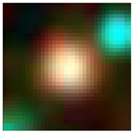
The image synthesis and preprocessing methods proposed by Pan et al. [14] were employed to enhance the quality and classification accuracy of galaxy images. The effectiveness of the methods was further demonstrated through an ablation study conducted by Pan et al. During the image synthesis process, the make_lupton_rgb function was used to combine the WISE data. Initially, the W1, W2, and W3 bands were normalized to ensure that the data from each band were fused on the same scale. The stretch factor of the make_lupton_rgb function was set to 0.5, and the brightness factor Q was set to 2. These parameter settings enhance the contrast and brightness of the images, thereby clarifying the details. The synthesized images effectively integrated information from different bands, providing a more comprehensive view of the celestial bodies. The results of the synthesis are illustrated in Figure 1.

To enhance the synthesized RGB image, we applied a non-local means denoising technique during the subsequent image preprocessing stage. This approach was selected to maintain the integrated context of the image by cohesively addressing noise characteristics across the combined bands. By denoising the RGB image, we ensured a unified treatment of noise across all channels, thus preserving both structural details and color information in the final composite. In the image preprocessing stage, a non-local means denoising technique was initially applied to effectively remove random noise while preserving important structural details. Subsequently, image enhancement techniques were employed to improve the contrast and sharpness of the images. These enhancements adjust the brightness and contrast, making the galaxy features more distinct and the images visually smoother. The results of these preprocessing steps are shown in Figure 2.

3. EWGC

3.1. Backbone—Efficient Former V2

A series of novel network structures, including VMamba, RMT, StarNet, EfficientFormerV2, etc., were evaluated on the galaxy morphology classification task, with the results presented in

Table 2. Comparison of experimental results for different networks (1).

Model	Accuracy (Test)	Spiral Precision	Spiral Recall	Spiral F1-Score	Elliptical Precision	Elliptial Recall	Elliptical F1-Score
EfficientFormerV2	89.79	88.93	89.88	89.41	90.59	89.70	90.14
RepViT	89.67	88.41	90.30	89.34	90.88	89.09	89.98
VMamba	88.53	88.44	87.50	87.97	88.60	89.47	89.03
RMT	88.68	88.11	88.32	88.21	89.22	89.02	89.12
StarNet	89.20	88.73	88.73	88.73	89.62	89.62	89.62
Efficientvit	88.84	88.27	88.49	88.38	89.37	89.17	89.27
EWGC	90.02	89.37	89.88	89.63	90.63	90.15	90.39

Note: bold entries in the table highlight the best results in each column. Note: underlined entries in the table highlight the second-best results in each column.

. As indicated in the table, EfficientFormerV2 demonstrated superior performance across all key metrics. Therefore, EfficientFormerV2 was selected as the foundational model for this study.

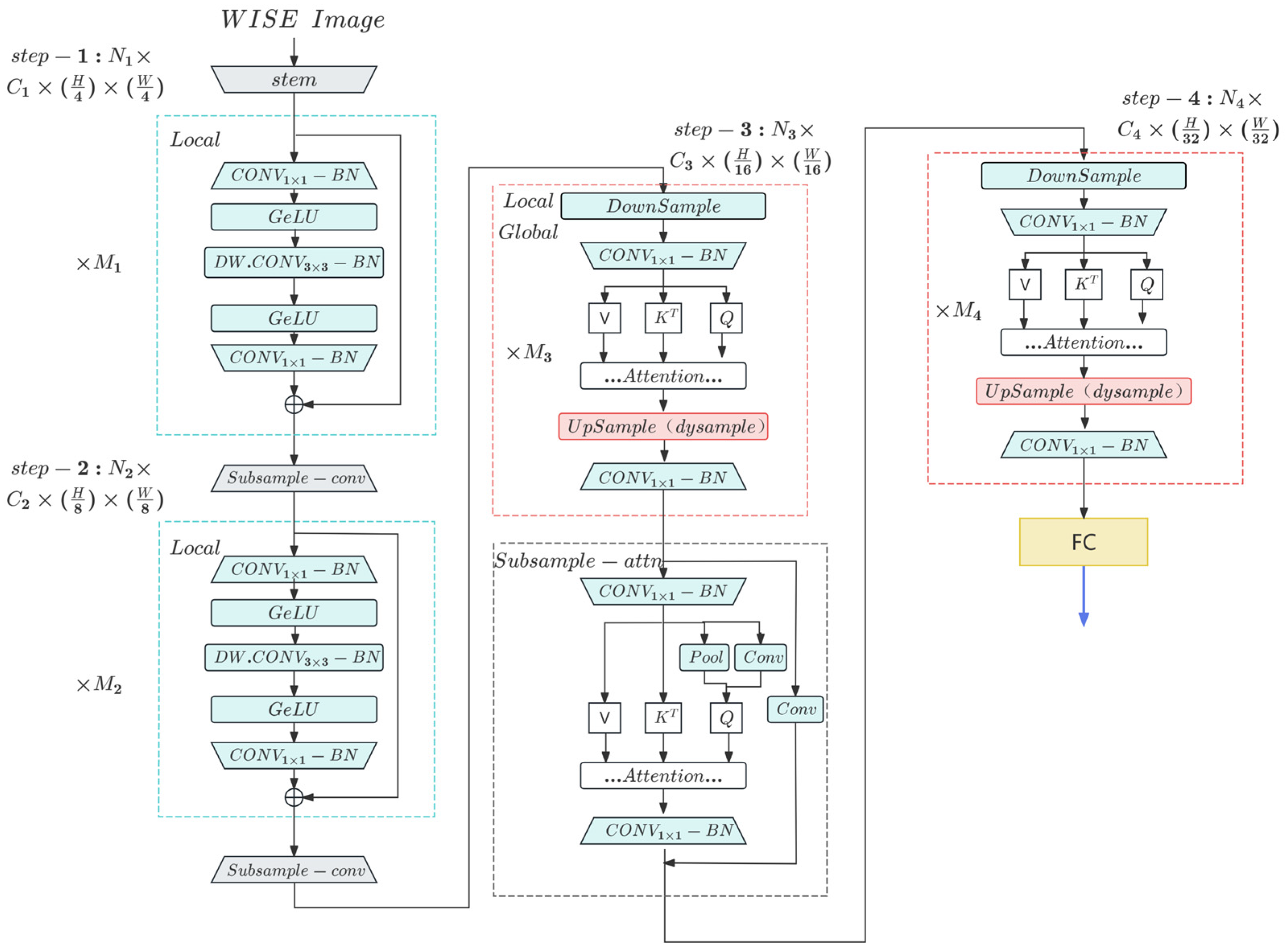
The EWGC, as illustrated in Figure 3, is designed based on the EfficientFormerV2 model. It efficiently extracts features from the input WISE images through a four-layered structure, achieving accurate classification while maintaining low latency and small model size.

In the first two stages of the model, the primary focus is on the extraction of local features. Deep convolution (DW.CONV) is used as the local token mixer. A new efficient FFN structure is formed by integrating the local token mixer (DW.CONV) and channel mixer (FFN) within the Transformer structure in the same residual structure. This modification enhances the performance without adding delay. Additionally, the downsampling is achieved through a 3 × 3 convolution with a stride of 2, aligning with the design concept of localized feature extraction.

The model shows improvement in classification accuracy metrics such as Area Under the Curve (AUC) and the Matthews Correlation Coefficient (MCC). The AUC of the Receiver Operating Characteristic (ROC) curve reflects the model’s overall ability to distinguish between classes, while the MCC provides a balanced measure of performance even with imbalanced classes, by calculating the correlation between observed and predicted classifications. At the same time, the false positive rate (FPR) of EWGC is reduced, the training efficiency is optimized while the training time is reduced, and the computational efficiency is improved by reducing the FLOPs and the number of covariates, achieving a more balanced model performance.

The latter two stages of the model primarily focus on the efficient fusion of global information, a key strength of the attention mechanism. EfficientFormerV2 incorporates an improved version of Attention for Higher Resolution Mechanisms and Dual-Path Attention downsampling for feature extraction and downsampling. To efficiently handle higher resolution inputs, EfficientFormerV2 introduces Stride Attention, which downscales the Query, Key, and Value tokens to a fixed resolution, significantly reducing computational complexity. Additionally, the Dual-Path Attentional downsampling mechanism combines static local downsampling with global dependency modeling to further enhance the accuracy. These two newly introduced attention mechanisms simultaneously utilize a new Multi-Head Self-Attention (MHSA) computation approach, including the infusion of local information into the value matrix using deep convolution (DW.CONV), and the communication of global information between heads using Talking Heads.

After the “2 + 2” local and global feature extraction process, the network achieves the classification task by utilizing a fully connected layer.

3.2. Lightweight Learnable Upsampling Framework—Dysample

In Efficient former v2, efficient global attention computation is achieved by performing downsampling before the attention mechanism, followed by upsampling at the end to restore the original image scale. Downsampling is typically implemented through a convolutional operation, which can be effectively tailored to the data characteristics during training. However, the upsampling process employs standard bilinear interpolation, often insufficient in accurately reconstructing feature maps. This limitation is particularly pronounced for small-scale targets (less than 34 × 34 pixels), such as those in this study, where inefficient upsampling can negatively impact classification accuracy. To address this issue, this work introduces a lightweight, learnable upsampling framework—Dysample [15]. The design specifics of the Dysample are described in the following (shown in Figure 4).

A simple implementation of the Dysample is illustrated in Figure 4a. Given a feature map of size $C\times H_1\times W_1$ and a sampling set of size $2\times H_2\times W_2$, the two in the first dimension denote the x and y coordinates. The grid_sample function resamples the hypothetical bilinearly interpolated X using the positions in S, generating an X′ of size $C\times H_2\times W_2$. This process is defined as follows:

$$X^{\prime }=\mathrm{grid}\_\mathrm{sample}(X,S)$$

(1)

provided an upsampling scale factor s and a feature map X of size $C\times H\times W$. A linear layer with input and output channels C and $2s^2$, respectively, is utilized to yield an offset O of size $2s^2\times H\times W$. Then, it is reshaped into $2\times sH\times sW$ using Pixel Shuffling. The sampling set S is then the sum of the offset O and the original sampling grid G, as follows:

$$O=linear(X)$$

(2)

$$S=g+O$$

(3)

Eventually, with the grid sample and sampling set S, an upsampled feature map of size $C\times sH\times sW$ can be created, as shown in Equation (1).

To enhance the accuracy of the initial sampling positions, a “static scope factor” is employed. In the original method, all the sampling locations were fixed at the same initial position, as shown in Figure 5a, which neglects the spatial relationships between neighboring points. To address this issue, the sampling process was refined using a “bilinear initialization” approach, as illustrated in Figure 5b. However, the overlap of sampling locations introduces prediction errors near the boundaries, which propagate incrementally, resulting in output artifacts. To mitigate this, the offset is multiplied by 0.25 to limit the displacement range of the sampling positions, as shown in Figure 5c. This “static range factor” effectively regulates the theoretical boundary conditions between overlapping and non-overlapping areas, ensuring a smoother and more precise sampling process. Accordingly, Equation (2) is rewritten as follows:

$$O=0.25linear(X)$$

(4)

3.3. EWGC_mag

Early releases of WISE data demonstrated that elliptical and spiral galaxies can be effectively distinguished through color–color diagrams, highlighting the critical role of magnitude information in the morphological classification of galaxies. The significance of this approach was further emphasized in the work of Pan et al. [14], where the integration of magnitude data proved beneficial. Building on this foundation, the present study investigates the potential of incorporating magnitude information to enhance image-based galaxy morphology classification. Building on this approach, the EWGC_mag network was designed to fuse image features with magnitude parameter features. As illustrated in Figure 6, the images are first processed to extract features, which are then flattened into a one-dimensional vector with 256 elements. Subsequently, the magnitude parameters (W1, W2, and W3) corresponding to each image are concatenated with this vector, resulting in a one-dimensional vector with 259 elements. This concatenated vector is finally input into a fully connected module for further processing.

4. Results

4.1. Evaluation Indicators

The performance of the classifier is comprehensively evaluated using the following metrics. Accuracy is the ratio of the number of correctly classified samples to the total number of samples. Precision is the ratio of the number of positive samples correctly predicted to the total number of positive samples predicted. Recall is the ratio of the number of samples correctly classified by the classifier to the number of actual positive samples out of all actual positive samples. F1-score is the reconciled average of precision and recall.

The formulas for accuracy, precision, recall, and F1-score are shown in Equations (5), (6), (7) and (8), respectively. In the formulas, TP refers to the number of instances where the model correctly predicted the positive class, TN refers to the number of instances where the model correctly predicted the negative class, FP refers to the number of instances where the model incorrectly predicted the positive class, and FN refers to the number of instances where the model incorrectly predicted the negative class.

$$\mathrm{Accuracy}={\displaystyle \frac{\mathrm{TP}+\mathrm{TN}}{\mathrm{TP}+\mathrm{TN}+\mathrm{FP}+\mathrm{FN}}}$$

(5)

$$\mathrm{Precision}={\displaystyle \frac{\mathrm{TP}}{\mathrm{TP}+\mathrm{FP}}}$$

(6)

$$\mathrm{Recall}={\displaystyle \frac{\mathrm{TP}}{\mathrm{TP}+\mathrm{FN}}}$$

(7)

$${\mathrm{F}}_1=2\times {\displaystyle \frac{\mathrm{precision}\times \mathrm{recall}}{\mathrm{precision}+\mathrm{recall}}}$$

(8)

In addition to standard performance metrics, three evaluation criteria are commonly used: floating point operations (FLOPs), number of parameters (params), and training time (Training Time (s)). FLOPs measure the total number of floating point operations required by the network, serving as a standard indicator of computational complexity. Params represent the total number of parameters that need to be trained in the network, providing insight into the model’s capacity and complexity. Training time refers to the duration required to complete a single epoch, representing the model’s training efficiency.

The experiments were conducted on hardware featuring an Intel Core i7-11700KF CPU and an NVIDIA GeForce RTX 3070Ti 8 GB GPU, with 16 GB of RAM. All networks were implemented using the PyTorch deep learning framework and the Python programming language.

4.2. Experimental Results and Verification

4.2.1. Verifying the Effectiveness of EWGC

The EWGC is compared with several novel networks, including VMamba, RMT, StarNet, and Efficientvit [16]. In this study, all networks were initialized and trained from scratch, without leveraging pre-trained weights. To facilitate binary classification, a fully connected layer comprising two output neurons was appended to the end of each model. These networks are designed to achieve state-of-the-art (SOTA) performance without additional tricks. All models were trained with identical hyperparameters and datasets to ensure convergence and consistency. The models were used from published codes without modifications for comparison. The EWGC demonstrates a superior balance between performance and computational efficiency (FLOPS), maintaining optimal performance with a moderate number of parameters and FLOPS.

The accuracy performance of the EWGC and its comparison network on the validation set is shown in Figure 7. The EWGC consistently demonstrated high accuracy throughout the training process, with accuracy levels stabilizing around 90%. In contrast, the accuracy of the other networks exhibited greater fluctuations, with WGC experiencing significant drops in accuracy at various training stages. Although EfficientFormerV2 and Efficientvit achieved higher accuracy, their performance was slightly less stable compared to EWGC. Furthermore, EWGC converged more quickly during the early training stages, with accuracy rising rapidly to a high level. Conversely, networks such as StarNet and VMamba exhibited relatively lower accuracy in the early training phases, indicating lower initial learning efficiency. Overall, EWGC shows notable advantages in both accuracy and stability.

From the comparison of the test set evaluation data (Table 2), the EWGC shows the highest overall accuracy at 90.02%, outperforming models such as EfficientFormerV2 (89.79%) and RepViT (89.67%). EWGC also delivers the strongest results in both spiral precision (89.37) and elliptical recall (90.15), which makes it particularly well-suited for galaxy classification.

The superior performance of EWGC is further highlighted through AUC, MCC, and FPR, as shown in

Table 3. Comparison of experimental results for different networks (2).

Model	AUC	MCC	Spiral FPR	Elliptocal FPR	Training Time (s)	FLOPs	Params
EfficientFormerV2	89.79	79.55	10.30	10.12	31.06	211.20 M	25.55 M
RepViT	89.69	79.34	10.91	9.70	28.21	378.59 M	22.41 M
VMamba	88.52	77.09	10.53	12.09	37.51	44.96 M	29.48 M
RMT	88.67	77.33	10.98	11.68	36.44	372.01 M	25.94 M
StarNet	89.18	78.35	10.38	11.27	15.63	86.64 M	7.48 M
Efficientvit	88.76	77.56	10.83	11.51	19.72	134.66 M	21.78 M
EWGC	90.02	80.02	9.85	10.12	29.09	210.91 M	25.73 M

Note: bold entries in the table highlight the best results in each column. Note: underlined entries in the table highlight the second-best results in each column.

. With an AUC of 90.02 and an MCC of 80.02, EWGC surpasses EfficientFormerV2 (AUC: 89.79, MCC: 79.55) and RepViT (AUC: 89.69, MCC: 79.34). While RepViT achieves a slightly lower false positive rate (FPR: 9.70), EWGC maintains competitive results with an FPR of 10.12, offering a balance between accuracy and precision. Models like VMamba and RMT show lower AUC (88.67, 77.33, respectively) and higher FPR, indicating a relative underperformance compared to the top contenders.

EWGC shows a significant superiority in training time, consuming only 29.09 s, which outperforms most other models, especially RepViT and RMT, demonstrating a faster training efficiency. The reduced time not only accelerates model development but also lowers resource consumption, contributing to its overall scalability in practical applications.

The computational overhead of EWGC, with FLOPs of 210.91 M and parameters totaling 25.73 M, remains comparable to EfficientFormerV2. This manageable overhead, coupled with the introduction of DySample, significantly enhances EWGC’s performance. Consequently, its optimized structure and classification precision establish EWGC as the most efficient and reliable model among those tested.

By comparing the performance of the EWGC, EfficientFormerV2, RepViT, VMamba, and RMT models, the EWGC model demonstrates strong accuracy overall but exhibits some misclassifications in specific cases. A closer examination reveals that misclassified spiral galaxy images often contain more background noise and interference from multiple objects, with complex surrounding colors, such as the intermingling of red and blue hues. In contrast, misclassified elliptical galaxy images tend to have less pronounced central brightness and blurred edges. Correctly classified elliptical galaxies, however, typically display bright white centers encircled by red regions. As illustrated in

Table 4. Example images of correct and incorrect classification.

	Spiral			Elliptical
Incorrect
Correct

, these examples of correct and misclassified galaxies highlight the features that influence classification accuracy, offering insights for future model refinement.

4.2.2. Validating the Effectiveness of the EWGC in Single and Multiple Object Galaxy Image Classification

The impact of contaminants from other sources on the classification of galaxies in WISE images was also assessed. The datasets were divided into two categories, “multiple” and “single”, based on analysis. “Multiple” refers to images that include objects other than the target galaxy, while “single” refers to images containing only the target galaxy.

Table 5. Example of single/multiple image in WISE.

	Spiral			Elliptical
Single
Mutiple

displays the example images of each category. By cross-matching within the image range using the TOPCAT software tool [17], the corresponding star table was derived, allowing for the determination of the presence of multiple targets in the images.

Table 6. Distribution of “single” and “multiple” types of data in the dataset.

	Train (Single–Multiple)	Validation (Single–Multiple)	Test (Single–Multiple)	Total (Single–Multiple)
Elliptical	3733:5230	1097:1471	613:707	5443:7408
Spiral	3940:4521	1094:1314	579:637	5593:6472

illustrates the distribution of the two types of data. Overall, the proportion of “single” to “multiple” is about 4:5. The categories of “single” and “multiple” are defined based on the 34 × 34 pixel images processed by the model. Images containing only a single-target are classified as “single”, while those containing multiple targets are classified as “multiple”.

The Grad-CAM [18] processed images for both types of data, visualizing the regions of focus of the model when dealing with single versus multiple objects; these images are shown in

Table 7. Example of WISE single/multiple images with Grad-CAM pre- and post-processing.

	Spiral		Elliptical
Single
Mutiple

. For single objects, the bright green areas clearly show that the model focuses mainly on the core region of the target galaxy. For multiple objects, the bright green area also shows that the model still focuses on the target galaxy, despite the presence of other objects in the image. EWGC is able to effectively deal with the interference of multiple objects and ensure the feature extraction of the target galaxy, demonstrating its robustness and anti-interference ability.

Each of the data subsets were tested individually and the respective results are detailed in

Table 8. Classification performance of EWGC on single/multiple test set.

Model	Accuracy	Spiral Precision	Spiral Recall	Spiral F1-Score	Elliptical Precision	Elliptial Recall	Elliptical F1-Score
Single	90.02	89.93	89.46	89.69	90.09	90.54	90.31
Multiple	90.03	88.87	90.26	89.56	91.10	89.82	90.46
Total	90.02	89.37	89.88	89.63	90.63	90.15	90.39

. The contrast analysis indicates that the EWGC can effectively classify the multiple objects within an image. This demonstrates the robustness of the model in handling images with multiple objects, as it successfully focuses on the main object in the center to ensure accurate classification. It is important to note that while multiple objects may not be physically related, the influence of WGC can potentially affect the classifier’s performance. Nevertheless, our model, EWGC, demonstrates a robust capability to mitigate this interference, thereby preserving classification accuracy.

4.2.3. Compare EWGC with EWGC_mag

Introducing galaxy magnitude information into the EWGC (i.e., EWGC_mag network) failed to significantly enhance classification performance, as shown in

Table 9. Classification performance of EWGC and EWGC_mag with magnitude information.

Model	Accuracy	Spiral Precision	Spiral Recall	Spiral F1-Score	Elliptical Precision	Elliptial Recall	Elliptical F1-Score
EWGC	90.02	89.37	89.88	89.63	90.63	90.15	90.39
EWGC_mag	90.18	89.53	90.05	89.79	90.78	90.30	90.54

. This contrasts with the WGC network, where incorporating galaxy magnitude information significantly improved classification accuracy by nearly 1%. The discrepancy can be attributed to the fact that magnitude information is inherently captured in the image data. The EWGC excels at extracting classification-relevant features from images, rendering the addition of extra magnitude information less impactful on performance enhancement.

Despite the limited performance gain, the fusion of magnitude features with image data in the EWGC_mag network remains a valuable experimental step. The goal was to determine whether incorporating explicit magnitude data could further enrich the feature space and improve classification accuracy. However, the results indicate that the added magnitude data are redundant, as the EWGC already captures these features directly from the images. This minimal impact highlights the powerful feature extraction capabilities of the network of networks, as its advanced feature extraction reduces dependence on supplementary data. Therefore, while the fusion step provided useful validation, it confirms that the EWGC architecture is already optimized for classification tasks without needing additional magnitude inputs.

5. Conclusions

The EWGC is introduced to classify spiral and elliptical galaxies. The study utilized a dataset comprising 12,088 spiral galaxies and 12,852 elliptical galaxies. This dataset was divided into a training set, a validation set, and a test set in the proportion of 7:2:1. The EWGC achieved a classification accuracy of 90.02% on the test set, with 89.37% accuracy for spiral galaxies and 90.63% for elliptical galaxies. Comparative tests with other classification networks confirmed the superior performance of the EWGC, particularly highlighting the effectiveness of its improvement module.

Additionally, the performance of the EWGC in “single” and “multiple” galaxy classification tasks is further analyzed. The results demonstrated that the EWGC maintains high classification accuracy even when processing complex images containing multiple celestial bodies. Following the principle of multimodal feature fusion, the EWGC_mag network was developed to combine WISE image features with magnitude features. While the overall classification accuracy did not significantly change from the original network, this design showcased the model’s capability to extract and utilize galaxy magnitude information.

To further enhance the accuracy of galaxy morphology classification, future work will focus on two key directions. First, deep generative models (e.g., variational autoencoders) will be explored to generate high-quality synthetic images, thereby expanding the dataset and improving the classification model’s performance. Second, incorporating spectral data will be considered to provide a more comprehensive analysis of the physical properties of galaxies. These efforts are expected to further improve the accuracy of galaxy classification and broaden the applicability of the models.

References

1. Neugebauer, G.; Habing, H.; Van Duinen, R.; Aumann, H.; Baud, B.; Beichman, C.; Beintema, D.; Boggess, N.; Clegg, P.; De Jong, T. The infrared astronomical satellite (IRAS) mission. Astrophys. J. 1984, 278, L1–L6, Part 2-Letters to the Editor (ISSN 0004-637X). [Google Scholar] [CrossRef]
2. Kessler, M.; Steinz, J.; Anderegg, M.; Clavel, J.; Drechsel, G.; Estaria, P.; Faelker, J.; Riedinger, J.; Robson, A.; Taylor, B. The infrared space observatory (ISO) mission. Astron. Astrophys. 1996, 315, L27–L31. [Google Scholar] [CrossRef]
3. Werner, M.W.; Roellig, T.L.; Low, F.; Rieke, G.H.; Rieke, M.; Hoffmann, W.; Young, E.; Houck, J.; Brandl, B.; Fazio, G. The Spitzer space telescope mission. Astrophys. J. Suppl. Ser. 2004, 154, 1. [Google Scholar] [CrossRef]
4. Wright, E.L.; Eisenhardt, P.R.; Mainzer, A.K.; Ressler, M.E.; Cutri, R.M.; Jarrett, T.; Kirkpatrick, J.D.; Padgett, D.; McMillan, R.S.; Skrutskie, M. The Wide-field Infrared Survey Explorer (WISE): Mission description and initial on-orbit performance. Astron. J. 2010, 140, 1868. [Google Scholar] [CrossRef]
5. Gardner, J.P.; Mather, J.C.; Clampin, M.; Doyon, R.; Greenhouse, M.A.; Hammel, H.B.; Hutchings, J.B.; Jakobsen, P.; Lilly, S.J.; Long, K.S. The james webb space telescope. Space Sci. Rev. 2006, 123, 485–606. [Google Scholar] [CrossRef]
6. Krizhevsky, A.; Sutskever, I.; Hinton, G.E. Imagenet classification with deep convolutional neural networks. Adv. Neural Inf. Process. Syst. 2012, 25. [Google Scholar] [CrossRef]
7. Simonyan, K.; Zisserman, A. Very deep convolutional networks for large-scale image recognition. arXiv 2014, arXiv:1409.1556. [Google Scholar]
8. Wang, A.; Chen, H.; Lin, Z.; Han, J.; Ding, G. Repvit: Revisiting mobile cnn from vit perspective. In Proceedings of the IEEE/CVF Conference on Computer Vision and Pattern Recognition, Seattle, WA, USA, 16–22 June 2024; pp. 15909–15920. [Google Scholar]
9. Gu, A.; Dao, T. Mamba: Linear-time sequence modeling with selective state spaces. arXiv 2023, arXiv:2312.00752. [Google Scholar]
10. Fan, Q.; Huang, H.; Chen, M.; Liu, H.; He, R. Rmt: Retentive networks meet vision transformers. In Proceedings of the IEEE/CVF Conference on Computer Vision and Pattern Recognition, Seattle, WA, USA, 16–22 June 2024; pp. 5641–5651. [Google Scholar]
11. Ma, X.; Dai, X.; Bai, Y.; Wang, Y.; Fu, Y. Rewrite the Stars. In Proceedings of the IEEE/CVF Conference on Computer Vision and Pattern Recognition, Seattle, WA, USA, 16–22 June 2024; pp. 5694–5703. [Google Scholar]
12. Li, Y.; Hu, J.; Wen, Y.; Evangelidis, G.; Salahi, K.; Wang, Y.; Tulyakov, S.; Ren, J. Rethinking vision transformers for mobilenet size and speed. In Proceedings of the IEEE/CVF International Conference on Computer Vision, Vancouver, BC, Canada, 17–24 June 2023; pp. 16889–16900. [Google Scholar]
13. Willett, K.W.; Lintott, C.J.; Bamford, S.P.; Masters, K.L.; Simmons, B.D.; Casteels, K.R.; Edmondson, E.M.; Fortson, L.F.; Kaviraj, S.; Keel, W.C. Galaxy Zoo 2: Detailed morphological classifications for 304 122 galaxies from the Sloan Digital Sky Survey. Mon. Not. R. Astron. Soc. 2013, 435, 2835–2860. [Google Scholar] [CrossRef]
14. Pan, Z.-R.; Qiu, B.; Liu, C.-X.; Luo, A.-L.; Jiang, X.; Guo, X.-Y. Morphological Classification of Infrared Galaxies Based on WISE. Res. Astron. Astrophys. 2024, 24, 045020. [Google Scholar] [CrossRef]
15. Liu, W.; Lu, H.; Fu, H.; Cao, Z. Learning to upsample by learning to sample. In Proceedings of the IEEE/CVF International Conference on Computer Vision, Vancouver, BC, Canada, 17–24 June 2023; pp. 6027–6037. [Google Scholar]
16. Liu, X.; Peng, H.; Zheng, N.; Yang, Y.; Hu, H.; Yuan, Y. Efficientvit: Memory efficient vision transformer with cascaded group attention. In Proceedings of the IEEE/CVF Conference on Computer Vision and Pattern Recognition, Vancouver, BC, Canada, 18–22 June 2023; pp. 14420–14430. [Google Scholar]
17. Taylor, M.B. TOPCAT & STIL: Starlink table/VOTable processing software. In Proceedings of the Astronomical Data Analysis Software and Systems XIV, Pasadena, CA, USA, 24–27 October 2004; p. 29. [Google Scholar]
18. Selvaraju, R.R.; Cogswell, M.; Das, A.; Vedantam, R.; Parikh, D.; Batra, D. Grad-CAM: Visual explanations from deep networks via gradient-based localization. In Proceedings of the IEEE International Conference on Computer Vision, Venice, Italy; 2017; pp. 618–626. [Google Scholar]
Figure 1. Examples of synthesized samples using make_lupton_rgb function. (a) Images of the WISE W1, W2, and W3 bands from left to right. (b) Image composition.
Universe 10 00394 g001
Figure 2. Example of image preprocessing. (a) Original image; (b) enhancement; (c) pixel map obtained by subtracting (a) from (b) for the composite map. (d) Pixel map of each channel map obtained by subtracting (a) from (b). From left to right, the first is the W1 channel, the second is the W2 channel, and the third is the W3 channel.
Universe 10 00394 g002
Figure 3. Diagram of EWGC: C is the number of channels, H is the height of the input image, W is the width of the input image, N is the number of input images, and M is the number of modules.
Universe 10 00394 g003
Figure 4. Sampling-based dynamic upsampling and module designs in Dysample. The input feature, upsampled feature, generated offset, and original grid are denoted by X, X′, O, and g, respectively. (a) The sampling set is generated by the sampling point generator, with which the input feature is re-sampled by the grid sample function. In generator (b), the sampling set is the sum of the generated offset and the original grid position. A version of the “static scope factor” is used, where the offset is generated with a linear layer.
Universe 10 00394 g004
Figure 5. Initial sampling positions and offset scopes. The points and the colored masks represent the initial sampling positions and the offset scopes, respectively. Considering sampling four points (s = 2), (a) in the case of nearest initialization, the four offsets share the same initial position but ignore position relation; in bilinear initialization (b), it separates the initial positions such that they distribute evenly. Without offset modulation (b), the offset scope would typically overlap, so in (c) it locally constrains the offset scope to reduce the overlap.
Universe 10 00394 g005
Figure 6. Diagram of EWGC_mag network. In line with the concept of multimodal feature fusion, the magnitude information from W1 to W3 is concatenated to the end of the flattened feature extracted using EWGC. A fully connected layer processes the fused multimodal information to perform the classification operation.
Universe 10 00394 g006
Figure 7. Accuracy of different model training and validation sets.
Universe 10 00394 g007