Abstract
This paper analyzes the rapid rendezvous trajectory of a spacecraft equipped with an advanced solar electric propulsion system towards asteroid 4660 Nereus. In this context, a set of possible minimum-time orbit-to-orbit transfer trajectories is calculated by modeling the propulsion system performance characteristics on those of NASA’s Evolutionary Xenon Thruster-Commercial (NEXT-C). In particular, the actual NEXT-C ion engine throttle table is used to calculate the optimal thrust control law that ensures the flight time is minimized for an assigned value for the spacecraft’s initial mass and the reference (electric) power at the beginning of the transfer. A baseline scenario that considers the actual inertial characteristics of the NASA’s DART spacecraft is analyzed in detail, and a parametric study is proposed to evaluate the transfer performance as a function of the main design parameters as, for example, the spacecraft’s initial mass and the reference power.
1. Introduction
Significant advances in ion thruster development over the past 25 years have contributed significantly to the planning of increasingly complex and ambitious missions, both in terms of achievable scientific goals and the ability to achieve more and better utilization of space resources [1]. So far, several missions using solar electric propulsion (SEP) as their main propulsion system have been carried out or are planned, including Deep Space 1, the first interplanetary mission propelled by SEP [2]; SMART-1, the first European mission to the Moon [3]; Dawn, the first mission to use SEP for a long-duration journey to explore Vesta and Ceres [4], and Psyche, to rendezvous with the largest metal asteroid in the solar system [5], to cite just a few.
The main reason for its success is that SEP makes many space missions attractive, as it can reduce the size of launch vehicles, and reduce the total propellant consumption, when compared with more conventional (i.e., chemical) propulsion systems. All this translates into significant mission cost savings [6]. The development of increasingly reliable SEP thrusters is also having an important impact from an economic point of view, making the concept of space resource exploitation increasingly advantageous, not only from an engineering perspective, but also from that of possible commercial investment. A first step in this direction is the recent missions that have demonstrated the possibility of extracting material from celestial bodies (usually near-Earth asteroids), collecting it, and returning it to Earth. Typical examples of asteroid mining include Hayabusa and its successor Hayabusa 2 and, more recently, OSIRIS-REx, which visited and collected a sample from asteroid 101955 Bennu [7,8,9]. These missions can be thought of as a first step towards a more ambitious goal of collecting large quantities of valuable substances that are hard to find on Earth, or even entire asteroids [10,11].
The starting point for studying the feasibility of reaching an asteroid is to design trajectories and analyze its accessibility considering commercial propulsion systems. Such a study is generally carried out using an optimal control approach, that is, minimizing an appropriate performance index, typically propellant mass, time of flight, or a combination of these two quantities [12]. Because the quality of the solution found is highly dependent on the mathematical model describing the operation of the thruster, it is important to use sufficiently accurate models to obtain reliable estimates of achievable performance. However, examples of studying optimal trajectories with realistic SEP throttle models are rarely addressed in the literature. An interesting approach in this regard is offered by the works of Taheri et al. [13,14], who studied the effects of a refined thrust model on the performance of a space mission.
In most cases the behavior of the SEP is mathematically described as a function of a single control variable, the input power to the power processing unit (PPU), which is assumed to be able to vary continuously over an assigned range of variation. Instead, since a SEP system has a finite number of operation points, the purpose of this paper is to evaluate the performance of an electric thruster with a realistic model, in which each operation point corresponds to given values of thrust, propellant mass flow rate, and PPU input power. In this regard, we updated a mathematical model, previously validated in other mission scenarios [15,16], by including the characteristics of a recent commercial-type propulsion system.
In particular, this paper analyzes minimum-time rendezvous trajectories to asteroid 4660 Nereus for a spacecraft equipped with a next-generation solar electric propulsion system. Asteroid 4660 Nereus, which approached Earth on 11 December 2011 with a minimum distance of about , has been considered in the past as a potential target for a robotic exploration mission [17,18], due to both its accessibility (in terms of delta-V) and its physical characteristics, which make it possible to maintain a closed orbit around such a small body in the solar system. It is classified as an E-type asteroid, possibly associated with aubrite meteorites, with a hight albedo (greater than 0.3) and a maximum diameter of [17] (see Figure 1).
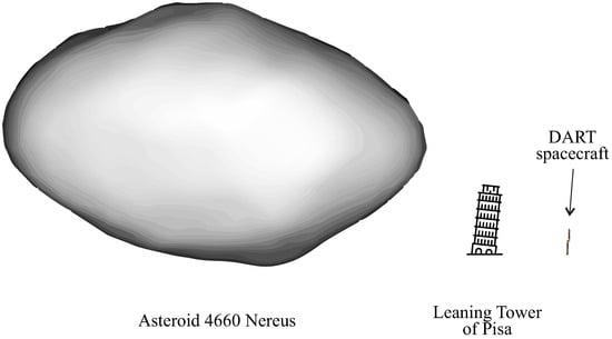
Figure 1.
Asteroid 4660 Nereus size comparison.
Its orbit, with an inclination of relative to the ecliptic plane, is illustrated in Figure 2.
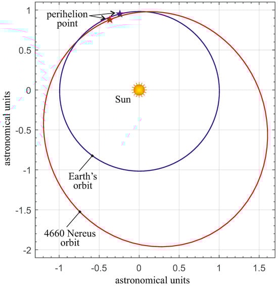
Figure 2.
Ecliptic projection of the asteroid 4660 Nereus orbit.
Assuming asteroid 4660 Nereus to be the primary target of a deep space exploration mission, a set of possible minimum-time orbit-to-orbit transfer trajectories is calculated by considering the performance characteristics of NASA’s Evolutionary Xenon Thruster-Commercial (NEXT-C) [19,20]. The latter is the propulsion system that was installed onboard the Double Asteroid Redirection Test (DART) spacecraft [21,22], which successfully completed its mission at the end of September 2022. Specifically, the acceleration table of the NEXT-C engine, together with a simplified analytical model of the performance of the power subsystem, is used to calculate the optimal control law that guarantees the minimization of the time of flight for an assigned value of the initial spacecraft mass and reference (electric) power. A baseline scenario that considers the actual inertial characteristics of the DART spacecraft is analyzed in detail, while a parametric study is proposed to evaluate transfer performance as a function of the spacecraft’s initial mass and reference power.
2. Mission Schematization and Mathematical Model Description
This section describes the mathematical model used to analyze the interplanetary mission scenario. Specifically, it illustrates the spacecraft dynamics model, the spacecraft thrust vector scheme, and the trajectory optimization process that was employed to obtain the numerical results. The mathematical approach is largely based on the model proposed by the authors in Ref. [15], where the interested reader can find a detailed discussion of the assumptions made. A simplified version of this model has also been used to study a circle-to-circle transfer to the inner regions of the solar system [16]. In this context, a novelty with respect to the model already presented in the literature [15] is the specific description of the characteristics of the propulsive system (i.e., the detailed table of thrusts), which is explained later in this section.
2.1. Spacecraft Dynamics in the Interplanetary Space
The spacecraft dynamics during the transfer are described by a simplified model, commonly used in the preliminary phase of interplanetary mission design. Specifically, the external forces acting on the spacecraft during flight consist of the gravitational pull of the Sun and the thrust provided by the on-board propulsion system. The latter can be set to zero by turning off the thruster, so that the transfer trajectory may include a coasting arc (i.e., a phase in which the spacecraft motion is purely Keplerian). Since the mass m of the spacecraft varies with time t and using a three-dimensional model for interplanetary transfer, the spacecraft state vector has 7 scalar components, i.e., the instantaneous mass of the vehicle and the 6 elements that define the position and velocity of the spacecraft. Following the common practice for trajectory analysis and optimization [23,24,25], the modified equinoctial orbit element set (MEOE) (An interesting discussion on the use of MEOEs can be found at the following link, retrieved on 10 September 2023: https://spsweb.fltops.jpl.nasa.gov/portaldataops/mpg/MPG_Docs/Source%20Docs/EquinoctalElements-modified.pdf) proposed by Walker et al. [26] was used to describe the spacecraft position and velocity. The relationships between the set of MEOEs and the classical orbital elements are as follows
where a is the semimajor axis, e is the eccentricity, i is the inclination, is the argument of perihelion, is the true anomaly, and is the right ascension of the ascending node of the spacecraft osculating orbit. Note that p coincides with the osculating orbit semilatus rectum, while the others MEOEs are dimensionless. The set of classical orbit elements can be recovered by inverting Equation (1), as described in Ref. [27], and the result is
Finally, the Sun-spacecraft distance r can be written as a function of MEOEs as
while the components of the spacecraft position and velocity vectors in a heliocentric-ecliptic (Cartesian) reference frame [28] of unit vectors can be obtained through the following relationships [23,29]
where is the Sun’s gravitational parameter.
Paralleling the procedure illustrated by Betts [29], and according to the model discussed in Ref. [15], the spacecraft state vector is defined as
so that the spacecraft dynamics is described by the vectorial equation
where is the electric thruster-induced propulsive acceleration vector, is a matrix whose entries depend on the MEOEs, while is a vector with two non-zero components only, which depend on both the propellant mass flow rate and a subset of MEOEs. In particular, according to Refs. [15,29] the expression of is
while the expression of is
The two propulsive terms and may be written as a function of the electric thruster characteristics, as described in the next subsection. Note that the components of the propulsive acceleration vector in Equation (7) are to be evaluated in a radial-tangential-normal (RTN) rotating reference frame whose unit vectors are defined as [29]
The RTN reference frame is schematized in Figure 3, which is an adaptation of a similar figure that has recently appeared in Ref. [27]. Note that the plane coincides with the plane of the spacecraft osculating orbit.
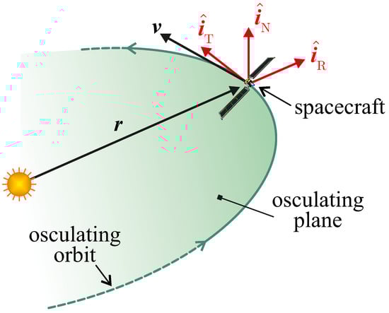
Figure 3.
Conceptual scheme of the rotating (RTN) reference frame with the unit vectors .
The initial condition required to complete the differential Equation (7) models the state of the spacecraft at the beginning of the interplanetary transfer, that is, at the initial time . In an orbit-to-orbit transfer, it is assumed that the spacecraft has an assigned initial mass
and that it initially travels through a Keplerian (parking) orbit with given characteristics. In this case, such a parking orbit coincides with Earth’s heliocentric orbit, so as to model a typical scenario in which the spacecraft leaves Earth’s sphere of influence with zero hyperbolic excess velocity relative to the planet [28]. The classical orbital elements describing the shape and orientation of the spacecraft osculating orbit at the initial time are obtained through the JPL Horizons system. Specifically, when using data from JPL Horizons (as of 1 August 2023), we have
Note that Equation (12) does not contain the value of the spacecraft’s initial true anomaly , because in a typical orbit-to-orbit transfer the angular position of the spacecraft along the parking orbit is left unconstrained and will be computed by solving an optimization problem, as described below. Likewise, the initial value of the true longitude L is left free, while the others elements are calculated by using Equations (1) and (12). In this case, the result is
The latter equation provides five (scalar) boundary constraints that will be used to complete the Two-Point Boundary Value Problem (TPBVP) associated with the optimization process described later in the section. Finally, the spacecraft’s mass at the beginning of the transfer must be considered as an assigned term (i.e., the value of is the sixth constraint of the TPBVP). In particular, the specific value of can be used to obtain the performance of the transfer parametrically.
2.2. Propulsive Characteristics and Thrust Vector Schematization
The propellant mass flow rate and the propulsive acceleration vector , i.e., the two “propulsive” terms that appear in the vector equation of motion (7), are usually modeled as a function of the on-board propulsion system. In this paper, the transfer performance is studied by considering an electric thruster modeled on the actual characteristics of the NEXT-C [30,31,32] that was installed aboard the DART spacecraft [22].
Specifically, the NEXT-C throttle table obtained from Refs. [33,34] was used to express the available thrust magnitude T, the nominal propellant mass flow rate , and the input power P to the PPU as a function of the throttle level , which is a (positive) integer indicating the possible operating point of the electric thruster. According to [33,34], the NEXT-C has 40 possible throttle levels, which are summarized in Table 1, where is a fictitious operating point that was introduced to model the electric thruster shutdown condition (in fact, gives a null value of T, P, and ).

Table 1.
Electric thruster throttle table adapted from the actual NEXT-C table.
The throttle table of the electric thruster used in the numerical simulations is also shown in Figure 4, where it can be seen that the maximum value of the thrust magnitude (i.e., ) is reached when and the input power is about with a propellant mass flow rate of about .
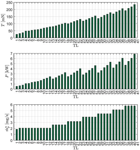
Figure 4.
Throttle table of the electric thruster used in the numerical simulations. The data are adapted from the actual table of the NEXT-C thruster.
In a spacecraft based on a solar electric propulsion system, i.e., one that uses solar panels to produce the electricity needed to power all on-board subsystems (including the thruster), the electric power available to drive the electric thruster can be approximated as the difference between the solar array output power and the power required by the other subsystems . The latter is considered in this paper to be a fixed (and assigned) value. Specifically, according to [15] the value of can be written as
so that when the solar array output power is less than the value of , the electric thruster is shut down by construction, i.e., the level is naturally selected; see Table 1. On the other hand, when the possible throttle levels that can be used to propel the spacecraft (at a generic point on the interplanetary trajectory) are those that satisfy the condition . A conceptual scheme of the electric power selection during the transfer is illustrated in Figure 5.
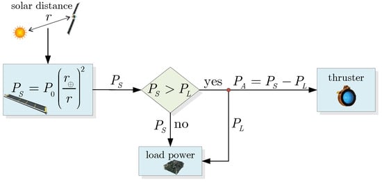
Figure 5.
Conceptual scheme of the electric power selection during the optimal transfer.
In Equation (14), the solar array output power is modeled with a simple function of the solar distance r and the reference power is defined as the solar array output power at the beginning of the life cycle and at a Sun-spacecraft distance , i.e.,
In particular, the value of is considered in this paper as assigned. Note that more refined mathematical models are presented in the literature to describe the variation of as a function of both solar distance and time (due to the degradation effect [35]), as discussed in Ref. [15]. In this context, an interesting historical approach is proposed in Refs. [6,36,37,38]. However, the simple model of Equation (15) is consistent with a preliminary trajectory design without introducing additional parameters that should be tailored to the specific power subsystem. Note that in this model the solar panels are always perpendicular to the incident sunlight.
The value of the propulsive acceleration vector and the (effective) propellant mass flow rate are obtained, as a function of TL, from the pair by introducing the duty cycle defined, according to [39], as the fraction of time during the deterministic thrust periods when the primary propulsive system is on. When using the duty cycle and the pair , we obtain
where is the unit vector of propulsive acceleration indicating the direction of the thrust vector induced by the electric thruster. The components in the rotating RTN frame of the unit vector can be expressed as a function of the two control angles and defined in Figure 6 as
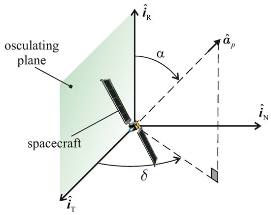
Figure 6.
Propulsive acceleration unit vector and thrust angles .
When taking into account the data summarized in Table 1 and Equation (16), the propulsive terms in the equations of motion (7) depend on the three dimensionless control variables . Accordingly, the throttle level and the two thrust angles are considered in this paper as the control parameters that can be used to design the interplanetary transfer trajectory. In particular, the control law, that is, the time variation of the triplet is determined by solving the optimization problem described in the next subsection.
2.3. Optimal Trajectory Design
The spacecraft transfer trajectory and the control law are obtained by studying an optimization problem in which the flight time is minimized. The spacecraft trajectory is determined so as to maximize the performance index , where is the final time when the spacecraft’s heliocentric orbit coincides with that of asteroid 4660 Nereus. This implies that the final value of the spacecraft true anomaly is not constrained. In fact, the final condition to be met is to obtain a final orbit whose orbital elements coincide with those of the target. By using again the JPL Horizons data at the 1 August 2023 we get
which can be rewritten in terms of MEOEs as
The flight time is minimized using an indirect approach [40,41], in which the costate vector is defined as
and the Hamiltonian function is obtained from Equations (7) and (20) as
from which the Euler-Lagrange equations are derived, viz.
The explicit expressions of the seven nonlinear differential equations that can be obtained from Equation (22) are omitted here for brevity.
The analytical form of the Hamiltonian function is used to find the optimal control law , , and . Indeed, according to the Pontryagin’s maximum principle [42], the optimal control law is the one that maximizes, at each instant of time t, the Hamiltonian function given by Equation (21). A standard procedure was employed to find the triplet that maximizes the local value of . The Hamiltonian function is also useful for writing the transversality condition that gives the following 4 boundary constraints
The TPBVP associated with the optimization process at an unspecified terminal time [40] is given by the 14 scalar differential Equations (7) and (22), with the 15 boundary constraints (recall that the flight time is an output of the process) given by Equations (11), (12), (18), and (23). The solution of the TPBVP, obtained by using the numerical approach used by the authors in [43,44], provides the optimal spacecraft trajectory and mission performance as a function of the duty cycle and the spacecraft design characteristics, i.e., initial mass , load power , and reference power . The numerical method used to solve the associated TPBVP is based on the use of a multiple shooting method [45] and a continuation procedure to extend the solution with for low computational cost. The numerical integration of the differential equations was performed using a standard numerical procedure based on the Adams–Bashforth method [46], with a relative and absolute tolerance of , whereas the TPBVP solution was obtained with an absolute tolerance of . The results of the numerical simulations are discussed in the next section.
3. Simulations and Numerical Results
Based on the mathematical model described in the previous section, the generic rapid transfer trajectory depends on the value of the set of design parameters . This section presents the numerical results of a series of simulations designed to assess the impact of the value of the design parameters on mission performance in terms of minimum flight time and required propellant mass .
Inder order to reduce the complexity of the numerical problem, a baseline scenario was assumed, in which the spacecraft characteristics were modeled on those of NASA’s DART spacecraft [21], with the exception of . More precisely, by taking into account the data presented in [47], a type of “reference spacecraft” was considered with an initial mass of , a reference power of , a load power of , and a duty cycle of . In this scenario, the solution of the optimization problem gives a minimum flight time of with a propellant mass consumption of . For comparative purposes, the DART spacecraft carried on board about of hydrazine propellant onboard for deep space maneuvers (and attitude control) and of xenon for the NEXT-C engine. As such, the total amount of propellant required to reach asteroid 4660 Nereus in this scenario, using a minimum time (orbit-to-orbit) transfer trajectory, is consistent with the total amount of propellant loaded on board the DART spacecraft. In this scenario, an optimal bi-impulsive orbit-to-orbit transfer trajectory, without ephemeris constraints, requires a minimum total velocity change of about with a corresponding flight time of . On the other hand, according to the CNEOS website (See the url retrieved in 23 October 2023: https://cneos.jpl.nasa.gov) a case using ephemeris constraints and a departure from a circular LEO with an altitude of requires a velocity change of about .
The solution of the optimal transfer problem gives the temporal variation of the spacecraft’s mass illustrated in Figure 7. Since the curve has a negative slope everywhere, it is evident that the propulsion system always remains on during the entire transfer. In other words, the optimal transfer trajectory contains no coasting arcs, that is, the (virtual) throttle level is never engaged.
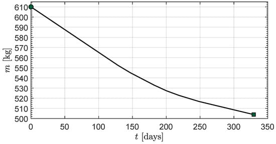
Figure 7.
Time variation of the spacecraft mass m in the baseline mission scenario. Green circle → start, green square → arrival.
This aspect is confirmed by the curves in Figure 8, which show the time variation of the optimal control law in terms of throttle level TL and thrust angles . Note, in the upper part of Figure 8, how the propulsion system engages the in the first phase of the transfer and then gradually reduces the throttle level according to the available electric power. The latter, in fact, decreases during the transfer because the solar array output power decreases with time due to the increase in Sun-spacecraft distance; see the spacecraft trajectory plotted in Figure 9. The initial phase with a constant value of TL is consistent with the time variation for the spacecraft’s mass shown in Figure 7, where the constant slope of the curve during the first of the transfer can be observed.
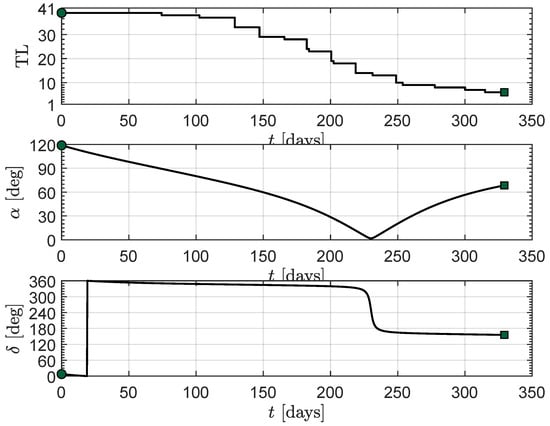
Figure 8.
Time variation of the optimal control law in the baseline mission scenario. Green circle → start, green square → arrival.
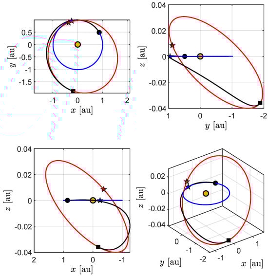
Figure 9.
Optimal transfer trajectory in the baseline mission scenario. See the text for the legend.
The optimal orbit-to-orbit transfer in the baseline scenario begins (or ends) when the spacecraft’s true anomaly is (or ), as confirmed by Figure 9, which shows the spacecraft transfer trajectory in a Cartesian heliocentric-ecliptic reference frame. In particular, Figure 9 shows the spacecraft trajectory (black line), the heliocentric orbit of the Earth (blue line) and asteroid (red line), the points of departure (black circle) and arrival (black square), the Sun (orange circle), and the perihelion points of the planetary orbits (blue and red stars). In this figure, the scale of the z-axis of the side and isometric views is expanded to better appreciate the three-dimensionality of the interplanetary transfer (recall that the asteroid orbit inclination is about ). Finally, the time variation of the classical orbital elements of the spacecraft’s osculating orbit are reported in Figure 10.
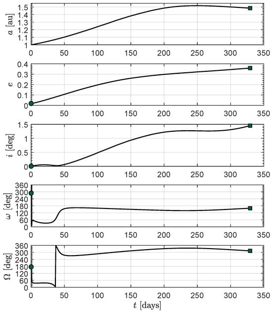
Figure 10.
Time variation of the osculating orbit classical orbital elements in the baseline mission scenario. Green circle → start, green square → arrival.
Transfer Performance Sensitivity
Transfer performance in the baseline mission scenario was used to evaluate the sensitivity of minimum flight time and propellant mass to a change in the design parameters . Specifically, each of the three parameters is designed to vary over an appropriate range in order to quantify the corresponding change in and .
For example, consider the case of ranging in the interval . When the values of the other design parameters are the same as those of the baseline scenario, the optimization process gives the results summarized in Figure 11. According to this figure, both the flight time and the propellant mass increase with . This is a rather expected result because a higher value of ( being fixed) gives a lower available power, which, in turn, changes the set of possible throttle levels in the engine performance of Table 1.
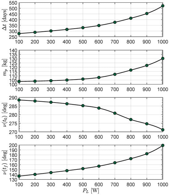
Figure 11.
Mission performance as a function of the value of , with , , and .
A thorough analysis of the effects of a variation in on mission performance is illustrated in Figure 12.
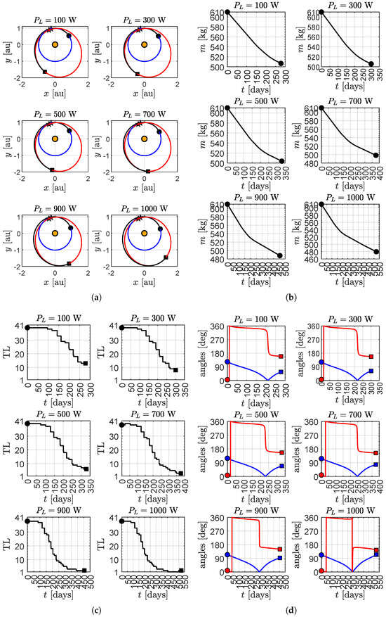
Figure 12.
Optimal trajectory, time variation with spacecraft mass and optimal control law as a function of the value of . (a) Trajectory ecliptic projection. (b) Mass variation with time. (c) Throttle level variation with time. (d) Thrust angles variation with time.
Similar trends are observed by varying the spacecraft’s initial mass or the reference electric power while keeping the other design parameters fixed (with a value equal to that used in the baseline scenario); see Figure 13. For example, a spacecraft with an initial mass of , , and is capable of completing the interplanetary transfer in less than with a propellant expenditure of about . On the other hand, a spacecraft with an initial mass of about twice the value used in the baseline scenario requires a flight time of about , which is nearly times the value obtained in the baseline scenario.
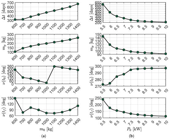
Figure 13.
Sensitivity analysis as a function of the value of and . (a) Case of varying . (b) Case of varying .
4. Final Remarks and Conclusions
Optimal trajectories to asteroid 4660 Nereus have been analyzed using data from a commercial-type electric propulsion system. By using a realistic dataset, namely the actual NEXT-C ion engine throttle table, it is possible to obtain the control law that minimizes the time of flight for an assigned value of the spacecraft’s initial mass and the electric power which are required at the beginning of the transfer. The simulations show that the transfer is feasible in a reasonable flight time, that is, less than one year and with a propellant mass consumption just over under the assumption of a load power of . This result is compatible with the propellant loaded on board the DART spacecraft, which used the same propellant system. The simulations are complemented by a thorough sensitivity study, in which the transfer performance was parameterized as a function of solar array output power, load power, and initial mass. The obtained results show that it is possible to have an accurate estimate of transfer times using a realistic thruster model.
Author Contributions
Conceptualization, A.A.Q.; methodology, A.A.Q.; software, A.A.Q.; writing—original draft preparation, A.A.Q., G.M. and M.B.; writing—review and editing, A.A.Q., G.M. and M.B. All authors have read and agreed to the published version of the manuscript.
Funding
This research received no external funding.
Institutional Review Board Statement
Not applicable.
Informed Consent Statement
Not applicable.
Data Availability Statement
Data are contained within the article.
Conflicts of Interest
The authors declare no conflict of interest.
Abbreviations
The following abbreviations are used in this manuscript:
| DART | Double Asteroid Redirection Test |
| MEOE | Modified Equinoctial Orbit Elements |
| NEXT-C | NASA’s Evolutionary Xenon Thruster - Commercial |
| PPU | Power Processing Unit |
| RTN | Radial-Tangential-Normal |
| SEP | Solar Electric Propulsion |
| TPBVP | Two-Point Boundary Value Problem |
The following symbols are used in this manuscript:
| a | semimajor axis [au] |
| propulsive acceleration vector [mm/s2] | |
| propulsive acceleration unit vector | |
| matrix, see Equation (8) | |
| vector, see Equation (9) | |
| e | orbital eccentricity |
| Hamiltonian function | |
| i | orbital inclination [deg] |
| radial unit vector | |
| transverse unit vector | |
| normal unit vector | |
| J | performance index [days] |
| m | spacecraft mass [kg] |
| propellant mass flow rate [kg/s] | |
| nominal propellant mass flow rate [kg/s] | |
| P | electric thruster input power [W] |
| solar array output power [W] | |
| available power [W] | |
| load power [W] | |
| MEOEs | |
| r | radial distance [au] |
| spacecraft position vector | |
| reference distance [] | |
| t | time [days] |
| T | thrust magnitude [N] |
| TL | throttle level |
| spacecraft velocity vector | |
| spacecraft state vector | |
| thrust pitch angle [rad] | |
| flight time [days] | |
| thrust clock angle [rad] | |
| generic adjoint variable to i-th state | |
| adjoint vector | |
| duty cycle | |
| Sun’s gravitational parameter [km3/s2] | |
| argument of periapse [deg] | |
| right ascension of the ascending node [deg] | |
| Subscripts | |
| 0 | initial, parking orbit |
| f | final, target orbit |
| Superscripts | |
| · | derivative with respect to time |
References
- Brophy, J. Advanced ion propulsion systems for affordable deep-space missions. Acta Astronaut. 2003, 52, 309–316. [Google Scholar] [CrossRef]
- Rayman, M.D.; Varghese, P.; Lehman, D.H.; Livesay, L.L. Results from the Deep Space 1 technology validation mission. Acta Astronaut. 2000, 47, 475–487. [Google Scholar] [CrossRef]
- Foing, B.; Racca, G.; Marini, A.; Evrard, E.; Stagnaro, L.; Almeida, M.; Koschny, D.; Frew, D.; Zender, J.; Heather, J.; et al. SMART-1 mission to the Moon: Status, first results and goals. Adv. Space Res. 2006, 37, 6–13. [Google Scholar] [CrossRef]
- Rayman, M.D.; Fraschetti, T.C.; Raymond, C.A.; Russell, C.T. Dawn: A mission in development for exploration of main belt asteroids Vesta and Ceres. Acta Astronaut. 2006, 58, 605–616. [Google Scholar] [CrossRef]
- Lord, P.; Tilley, S.; Oh, D.Y.; Goebel, D.; Polanskey, C.; Snyder, S.; Carr, G.; Collins, S.M.; Lantoine, G.; Landau, D.; et al. Psyche: Journey to a metal world. In Proceedings of the 2017 IEEE Aerospace Conference, Big Sky, MT, USA, 4–11 March 2017. [Google Scholar] [CrossRef]
- Williams, S.N.; Coverstone-Carroll, V. Benefits of Solar Electric Propulsion for the Next Generation of Planetary Exploration Missions. J. Astronaut. Sci. 1997, 45, 143–159. [Google Scholar] [CrossRef]
- Sankaran, K.; Hamming, B.; Grochowski, C.; Hoff, J.; Spaun, M.; Rollins, M. Evaluation of Existing Electric Propulsion Systems for the OSIRIS-REx Mission. J. Spacecr. Rocket. 2013, 50, 1292–1295. [Google Scholar] [CrossRef]
- Sutter, B.; Hatten, N.; Getzandanner, K.M.; Hughes, K.M.; Wibben, D.; Williams, K.; Moreau, M.C.; Englander, J.; Mudek, A.J.; Lauretta, D.; et al. OSIRIS-REx Extended Mission Trajectory Design and Target Search. In Proceedings of the AIAA SCITECH 2022 Forum, San Diego, CA, USA, 3–7 January 2022. [Google Scholar] [CrossRef]
- Burke, K.N.; DellaGiustina, D.N.; Bennett, C.A.; Walsh, K.J.; Pajola, M.; Bierhaus, E.B.; Nolan, M.C.; Boynton, W.V.; Brodbeck, J.I.; Connolly, H.C.; et al. Particle Size-Frequency Distributions of the OSIRIS-REx Candidate Sample Sites on Asteroid (101955) Bennu. Remote Sens. 2021, 13, 1315. [Google Scholar] [CrossRef]
- Brophy, J.; Oleson, S. Spacecraft Conceptual Design for Returning Entire Near-Earth Asteroids. In Proceedings of the 48th AIAA/ASME/SAE/ASEE Joint Propulsion Conference & Exhibit, Atlanta, GA, USA, 29 July–1 August 2012. [Google Scholar] [CrossRef][Green Version]
- Mazanek, D.D.; Merrill, R.G.; Brophy, J.R.; Mueller, R.P. Asteroid Redirect Mission concept: A bold approach for utilizing space resources. Acta Astronaut. 2015, 117, 163–171. [Google Scholar] [CrossRef]
- Mengali, G.; Quarta, A.A. Optimal trade studies of interplanetary electric propulsion missions. Acta Astronaut. 2008, 62, 657–667. [Google Scholar] [CrossRef]
- Taheri, E.; Junkins, J.L.; Kolmanovsky, I.; Girard, A. A novel approach for optimal trajectory design with multiple operation modes of propulsion system, part 2. Acta Astronaut. 2020, 172, 166–179. [Google Scholar] [CrossRef]
- Nurre, N.P.; Taheri, E. Duty-cycle-aware low-thrust trajectory optimization using embedded homotopy. Acta Astronaut. 2023, 212, 630–642. [Google Scholar] [CrossRef]
- Quarta, A.A.; Mengali, G. Minimum-Time Space Missions with Solar Electric Propulsion. Aerosp. Sci. Technol. 2011, 15, 381–392. [Google Scholar] [CrossRef]
- Quarta, A.A.; Izzo, D.; Vasile, M. Time-Optimal Trajectories to Circumsolar Space Using Solar Electric Propulsion. Adv. Space Res. 2013, 51, 411–422. [Google Scholar] [CrossRef]
- Brozovic, M.; Ostro, S.; Benner, L.; Giorgini, J.; Jurgens, R.; Rose, R.; Nolan, M.; Hine, A.; Magri, C.; Scheeres, D.; et al. Radar observations and a physical model of Asteroid 4660 Nereus, a prime space mission target. Icarus 2009, 201, 153–166. [Google Scholar] [CrossRef]
- Kawaguchi, J.; Fujiwara, A.; Sawai, S. Sample and return mission from asteroid Nereus via solar electric propulsion. Acta Astronaut. 1996, 38, 87–101. [Google Scholar] [CrossRef]
- Fisher, J.; Ferraiuolo, B.; Monheiser, J.; Goodfellow, K.; Hoskins, A.; Myers, R.; Bontempo, J.; McDade, J.; O’malley, T.; Soulas, G.; et al. NEXT-C flight ion system status. In Proceedings of the AIAA Propulsion and Energy 2020 Forum, Virtual Event, 24–28 August 2020. [Google Scholar] [CrossRef]
- Monheiser, J.; Goodfellow, K.; Aubuchon, C.; Wang, J.; Ferraiuolo, B.; Williams, G.; Soulas, G.; Shastry, R.; Arthur, N. A Summary of the NEXT-C Flight Thruster Proto-flight Testing. In Proceedings of the AIAA Propulsin and Energy Forum, Virtual, 11–14 August 2021. [Google Scholar] [CrossRef]
- Adams, E.; Oshaughnessy, D.; Reinhart, M.; John, J.; Congdon, E.; Gallagher, D.; Abel, E.; Atchison, J.; Fletcher, Z.; Chen, M.; et al. Double Asteroid Redirection Test: The Earth Strikes Back. In Proceedings of the 2019 IEEE Aerospace Conference, Big Sky, MT, USA, 2–9 March 2019. [Google Scholar] [CrossRef]
- John, J.; Roufberg, L.; Ottman, G.K.; Adams, E. NEXT-C Lessons Learned on the DART Mission for Future Integration and Test. In Proceedings of the 2023 IEEE Aerospace Conference, Big Sky, MT, USA, 4–11 March 2023. [Google Scholar] [CrossRef]
- Coverstone, V.L.; Prussing, J.E. Technique for Escape from Geosynchronous Transfer Orbit Using a Solar Sail. J. Guid. Control Dyn. 2003, 26, 628–634. [Google Scholar] [CrossRef]
- Kechichian, J. Trajectory optimization with a modified set of equinoctial orbit elements. In Proceedings of the AAS/AIAA Astrodynamics Specialist Conference, Durango, CO, USA, 19–22 August 1991. [Google Scholar]
- Pontani, M. Optimal Space Trajectories with Multiple Coast Arcs Using Modified Equinoctial Elements. J. Optim. Theory Appl. 2021, 191, 545–574. [Google Scholar] [CrossRef]
- Walker, M.J.H.; Ireland, B.; Owens, J. A set of modified equinoctial orbit elements. Celest. Mech. 1985, 36, 409–419, Erratum in Celest. Mech. 1986, 38, 391–392. [Google Scholar] [CrossRef]
- Quarta, A.A.; Abu Salem, K.; Palaia, G. Solar sail transfer trajectory design for comet 29P/Schwassmann-Wachmann 1 rendezvous. Appl. Sci. 2023, 13, 9590. [Google Scholar] [CrossRef]
- Bate, R.R.; Mueller, D.D.; White, J.E. Fundamentals of Astrodynamics; Dover Publications: New York, NY, USA, 1971; Chapter 2; pp. 53–55, 368–372. [Google Scholar]
- Betts, J.T. Very low-thrust trajectory optimization using a direct SQP method. J. Comput. Appl. Math. 2000, 120, 27–40. [Google Scholar] [CrossRef]
- Shastry, R.; Soulas, G.; Aulisio, M.; Schmidt, G. Current status of NASA’S NEXT-C ion propulsion system development project. In Proceedings of the 68th International Astronautical Congress, IAC, Adelaide, Australia, 25–29 September 2017. [Google Scholar]
- Overton, S.; Jackson, J.; Spores, R.; Kelleher, K.; Allen, M.; Hertel, T.; Hoskins, A. GN&C applications using next generation NEXT-C high power ion thruster. In Proceedings of the 39th Annual AAS Rocky Mountain Section Guidance and Control Conference, Breckenridge, CO, USA, 5–10 February 2016; Volume 157, pp. 839–849. [Google Scholar]
- Aulisio, M.; Pinero, L.; White, B.; Hickman, T.; Bontempo, J.; Hertel, T.; Birchenough, A. Status of the development of flight power processing units for the NASA’s evolutionary Xenon Thruster—Commercial (NEXT-C) project. In Proceedings of the 14th International Energy Conversion Engineering Conference, Salt Lake City, UT, USA, 25–27 July 2016. [Google Scholar] [CrossRef]
- NASA’s Evolutionary Xenon Thruster (NEXT) Ion Propulsion GFE Component Information Summary for Discovery Missions July 2014. Nasa Discovery Program Announcement of Opportunity Program Library, NASA. 2014. Available online: http://discovery.larc.nasa.gov/discovery/pdf_files/20-NEXT-C_AO_Guidebook_11July14.pdf (accessed on 24 October 2023).
- NEXT-C Ion Propulsion System (IPS) Information Summary for New Frontiers Missions. Technical Report, NASA; 2017. Available online: https://newfrontiers.larc.nasa.gov/NF4/PDF_FILES/NEXT-C_New_Frontiers_Guidebook_20161230_REV5.pdf (accessed on 24 October 2023).
- Kerslake, T.; Gustafson, E. On-Orbit Performance Degradation of the International Space Station P6 Photovoltaic Arrays. In Proceedings of the 1st International Energy Conversion Engineering Conference (IECEC), Portsmouth, NH, USA, 15–17 August 2003. [Google Scholar] [CrossRef][Green Version]
- Sauer, C.G., Jr.; Bourke, R. The effect of solar array degradation on electric propulsion spacecraft performance. In Proceedings of the 9th Electric Propulsion Conference, Bethesda, MD, USA, 17–19 April 1972. [Google Scholar] [CrossRef]
- Sauer, C.G., Jr. Modeling of thruster and solar array characteristics in the JPL low-thrust trajectory analysis. In Proceedings of the 13th International Electric Propulsion Conference, San Diego, CA, USA, 27–27 April 1978. [Google Scholar] [CrossRef]
- Woo, B.; Coverstone, V.L.; Hartmann, J.W.; Cupples, M. Trajectory and System Analysis For Outer-Planet Solar Electric Propulsion Missions. J. Spacecr. Rocket. 2005, 42, 510–516. [Google Scholar] [CrossRef]
- Rayman, M.D.; Williams, S.N. Design of the First Interplanetary Solar Electric Propulsion Mission. J. Spacecr. Rocket. 2002, 39, 589–595. [Google Scholar] [CrossRef]
- Bryson, A.E.J.; Ho, Y.C. Applied Optimal Control; Hemisphere Publishing Corporation: New York, NY, USA, 1975. [Google Scholar]
- Stengel, R.F. Optimal Control and Estimation; Dover Publications: Mineola, NY, USA, 1994; pp. 222–254. [Google Scholar]
- Ross, I.M. A Primer on Pontryagin’s Principle in Optimal Control; Collegiate Publishers: San Francisco, CA, USA, 2015; Chapter 2; pp. 127–129. [Google Scholar]
- Mengali, G.; Quarta, A.A. Optimal three-dimensional interplanetary rendezvous using nonideal solar sail. J. Guid. Control Dyn. 2005, 28, 173–177. [Google Scholar] [CrossRef]
- Mengali, G.; Quarta, A.A. Fuel-optimal, power-limited rendezvous with variable thruster efficiency. J. Guid. Control Dyn. 2005, 28, 1194–1199. [Google Scholar] [CrossRef]
- Yang, W.Y.; Cao, W.; Kim, J.; Park, K.W.; Park, H.H.; Joung, J.; Ro, J.S.; Hong, C.H.; Im, T. Applied Numerical Methods Using MATLAB®; John Wiley & Sons, Inc.: Hoboken, NJ, USA, 2020; Chapters 6–7; pp. 333–336, 376–378. [Google Scholar]
- Shampine, L.F.; Reichelt, M.W. The MATLAB ODE Suite. SIAM J. Sci. Comput. 1997, 18, 1–22. [Google Scholar] [CrossRef]
- Sarli, B.V.; Atchison, J.A.; Ozimek, M.T.; Englander, J.A.; Barbee, B.W. Double Asteroid Redirection Test Mission: Heliocentric Phase Trajectory Analysis. J. Spacecr. Rocket. 2019, 56, 546–558. [Google Scholar] [CrossRef]
Disclaimer/Publisher’s Note: The statements, opinions and data contained in all publications are solely those of the individual author(s) and contributor(s) and not of MDPI and/or the editor(s). MDPI and/or the editor(s) disclaim responsibility for any injury to people or property resulting from any ideas, methods, instructions or products referred to in the content. |
© 2023 by the authors. Licensee MDPI, Basel, Switzerland. This article is an open access article distributed under the terms and conditions of the Creative Commons Attribution (CC BY) license (https://creativecommons.org/licenses/by/4.0/).