Abstract
The evolution of hard probes in a medium is a complex multiscale problem that significantly benefits from the use of Effective Field Theories (EFTs). Within the EFT framework, we aim to define a series of EFTs in a way that addresses each energy scale individually in separate steps. However, studying hard probes in a medium presents challenges. This is because an EFT is typically constructed by formulating the most general Lagrangian compatible with the problem’s symmetries. Nevertheless, medium effects may not always be encoded adequately in an effective action. In this paper, we construct an EFT that is valid for studying the evolution of a heavy quark in a QCD plasma containing few other heavy quarks, where degrees of freedom with an energy of the order of the temperature scale are integrated out. Through this example, we explicitly demonstrate how to handle the doubling of degrees that arise in non-equilibrium field theory. As a result, we derive a Fokker–Planck equation using only symmetry and power counting arguments. The methods introduced in this paper will pave the way for future developments in the study of quarkonium suppression.
1. Introduction
Quark–gluon plasma is a state of matter that forms at high temperatures and densities, in which quarks and gluons are not confined within hadrons. This state of matter can be created on Earth in experiments using ultrarelativistic heavy-ion collisions. However, quark–gluon plasma exists only for a very short time during these collisions, so we must study the particles produced during this brief period to learn about the properties of the plasma. One approach is to study “hard probes”, which are observables that are both significantly affected by the medium and can be measured in the challenging environment of a heavy-ion collision. Examples of hard probes include heavy quarks, heavy quarkonium, and jets.
Studying heavy particles and jets in a medium requires dealing with largely separated energy scales. Particles with energies of the order of the heavy quark mass or a hard parton energy are rare in the medium and can be accurately described using perturbative QCD. However, particles with energies of the order of the temperature are sensitive to the medium and cannot always be described using perturbation theory. Therefore, it is interesting to separate the contribution from these two kind of particles to encode non-perturbative effects in parameters or functions that can be computed using non-perturbative methods like lattice QCD. It is also important to be careful when describing systems with largely separated energy scales. On one hand, the appearance of largely separated energy scales can lead to a breaking of naive perturbation theory, meaning that the size of a contribution cannot be directly related to its number of loops. On the other hand, non-perturbative studies using lattice QCD are also challenging because a very large lattice is required to accommodate all the energy scales.
These problems can be solved by using EFTs. An EFT is a quantum field theory that gives the same results as another more general theory at low energies. They are constructed in the following way [1]:
- Identify the relevant degrees of freedom and the symmetries of the problem.
- Write the more general Lagrangian that respects the symmetries of the problem using the relevant degrees of freedom.
- An EFT must be equipped with a power counting. This means that there is a simple rule to predict how large the contribution is of each term in the Lagrangian for a given observable.
- The unknown parameters in the effective Lagrangian are called Wilson coefficients. They are fixed by imposing that the EFT gives the same results as the full theory at low energies. This procedure is called matching.
Note that an EFT Lagrangian has an infinite number of terms. However, the theory still has predictive power thanks to the power counting.
The use of EFTs can also allow relating physical observables with quantities computable on the lattice in a more direct way. A good example is the description of heavy quarkonium. Heavy quarkonium is a bound state made of a heavy quark and a heavy antiquark. Quarkonium is a non-relativistic system in which well-separated energy scales appear. They are the mass, M, the inverse of the typical radius, with , and the binding energy . Non-relativistic QCD (NRQCD) [2,3] is an EFT valid for energies smaller than M. Since , we can reliably match QCD to NRQCD using perturbation theory. We can also use Potential NRQCD (pNRQCD) [4,5,6], an EFT valid for energies much smaller than . Since this scale is not always perturbative, there are cases in which the matching between NRQCD and pNRQCD cannot be done in perturbation theory. However, since each term in the pNRQCD Lagrangian has a scaling with that is easy to determine, we can perform the matching between NRQCD and pNRQCD in the limit in which the mass of the heavy quarks is infinite (the static limit). Once the matching is carried out, we can use these Wilson coefficients to compute the properties of quarkonium states with finite heavy quark masses. This is a rigorous way of showing that the spectrum of quarkonium can be determined by solving a Schrödinger equation in which the potential is computed on the lattice using static quarks.
EFTs have been applied to the study of hard probes in heavy-ion collisions. In the case of heavy quarkonium, medium modified versions of NRQCD and pNRQCD have been used to compute the thermal corrections to the mass and the medium-induced decay width [7,8,9]. pNRQCD has also been used to study the evolution of the population of bound states inside of a medium in the cases in which [10,11,12,13]. Regarding jets, there are recently developed EFTs for the study of jet broadening in [14] as well as jet sub-structures in heavy-ion collisions [15].
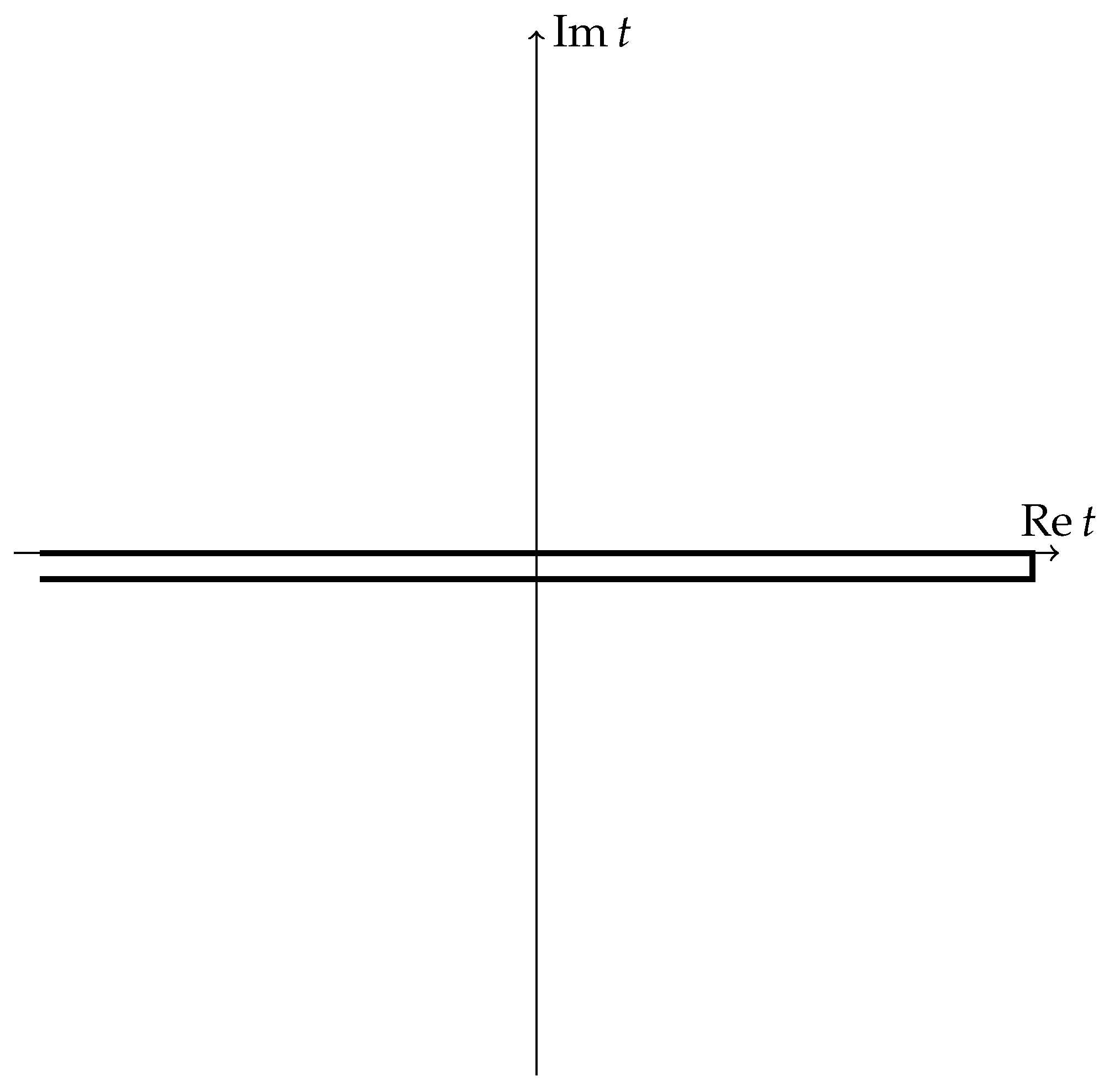
However, the application of the EFT framework to the study of hard probes in a medium presents a conceptual challenge. The procedure that we have outlined before needs to be modified when the medium affects the matching between the full theory and the EFT. At a finite temperature, computations of non-static properties are performed using so-called real-time formalism [16]. In this formalism, there is a doubling of the degrees of freedom. This means that the standard path integral has to be substituted by a path integral in which the time integration follows the complex Schwinger-Keldysh contour (see Figure 1). In practice, instead of considering explicitly the complex–time integration, we name fields with a time argument on the upper (lower) branch of the contour fields of type 1(2). As an example, let us consider a QFT describing the evolution of a field . Then, the action can be written as
where the subindex C means that the integration is performed along the Schwinger-Keldysh contour. In this way, due to the properties of the path integral, correlators in which only fields of type 1(2) appear are chronologically (anti-chronologically) ordered. However, we might be interested in evaluating correlators that are neither chronologically nor anti-chronologically ordered. For example, if we want to gain access to the distribution function, we would need to compute , where the ordering of the operators is as written. Note also that, although in Equation (1) there are no terms containing, at the same time, both types of fields, the propagator of the field is not diagonal in the indices [16].

Figure 1.
Representation of the Schwinger-Keldysh contour. The thicker line represents the complex time contour along which the path integral is defined in non-equilibrium field theory. It goes from to ∞ and then goes back to but decreases the time’s imaginary part by an infinitely small amount.
What we have explained up until now regarding the Schwinger-Keldysh contour (for the specific case of a QFT describing the evolution of a field ) is standard textbook material. However, it is important to recall this information in order to highlight non-trivial features that appear when we apply the EFT framework to a non-equilibrium or thermal field theory. When we integrate out degrees of freedom, the matching between the full theory and the EFT might induce terms including the two types of fields. In other words, the EFT might not show the structure that appears in Equation (1). Physically, we might interpret this in the following way. The EFT describes the evolution of an open quantum system interacting with an environment (the medium degrees of freedom that have been integrated out). It is a well-known result in quantum mechanics that the evolution of an open quantum system cannot be encoded in a Hamiltonian [17]. In other words, in general, an operator does not exist, such that the time-evolution of the density matrix can be written as a von-Neumann equation. Instead, the evolution of the density matrix of a open quantum system follows a more general kind of equation. The same is true if we apply path integral formalism. The effect of high-energy fields on low-energy ones can not be encoded into an effective action when we are dealing with an open quantum system. We need a more general object, called a influence functional, instead [18]. For the example of a field
where means ordering along the Schwinger-Keldysh contour and is the influence functional. Only in the case of an isolated system does , where S is the effective action.
Taking this into account is a substantial modification of the second point of the procedure we outlined to construct an EFT. Up until now, this difficulty has been skipped in the study of hard probes using two different strategies. The first one is to focus on computing the binding energy and the decay width of non-relativistic systems. In this case, the effects of the doubling of the degrees of freedom are neutralized in the approximation in which the heavy particles are diluted [7,8]. The second strategy is to study cases in which the temperature is smaller than the energies that are integrated out to define the EFT [10,11].
The construction of EFTs that do not consist in an effective action has been investigated in the context of the development of an EFT for hydrodynamics [19,20,21,22]. However, to our knowledge, these developments have not been applied to the study of hard probes in a QCD plasma. In this manuscript, we aim to fill this gap by studying a simple example: a heavy quark close to thermalization in a medium with few other heavy quarks. In this problem, we can identify three widely separated energy scales.
- The mass of the heavy quark M.
- The spatial momentum of the heavy quark p, which is of the order of , with T being the temperature.
- The temperature T and other energy scales that the medium might induce.
It is well known that this situation can be studied using a Fokker–Planck equation or the physically equivalent Langevin equation [23,24,25,26,27,28,29]. In this manuscript, we will give an EFT perspective on the problem. Following the EFT philosophy, we will deal with each energy scale in a separate way. We will follow the following steps:
- As a starting point, we can use NRQCD. This automatically encodes the effects of the degrees of freedom with an energy of order M.
- It is straight-forward to define an EFT for energies smaller than . This EFT is a modification of NRQCD using the momentum label technique common in Soft-Collinear Effective Theory (SCET) [30,31] and On-Shell Effective Theory (OSEFT) [32,33]. An equivalent EFT, with the same degrees of freedom, symmetries, and power counting, was previously introduced to study a completely different problem. This is an NRQCD for semi-hard fields () [34]. This EFT was originally introduced to study modes with an energy of the order in the study of heavy quarkonium at . In our case, the role of is played by T. However, symmetries and power counting arguments remain the same.
- We define an EFT for energies below T. In this EFT, there are terms that mix fields of type 1 and type 2. These are dealt with following the approach of [19] but supplementing it with the properties of the dilute expansion. We call this EFT Langevin Effective Theory (LET) due to its connection with the Langevin equation.
- We perform the matching between and LET in the one-gluon exchange approximation as an illustration. This allows us to encode the influence of the degrees of freedom with an energy of order T.
- We use LET to compute the evolution of the density of heavy quarks, obtaining a Fokker–Planck equation for the density that coincides with the evolution resulting from a Langevin equation.
This procedure could seem extremely complex to obtain results that are already well-known. However, our aim is to develop techniques that could be useful for more interesting cases. In particular, we have in mind the study of the evolution of the reduced density matrix of quarkonium in the regime . The problem that we study in this manuscript is simpler than quarkonium in the regime . However, in both cases we are dealing with dilute non-relativistic particles. One important observation that the framework developed here makes manifest is that the physics at the scale T can be studied in the static limit. In other words, the matching between and LET can be done in the static limit, and we can use those Wilson coefficients to study the finite M case. A similar thing happens regarding the matching between NRQCD and pNRQCD at . These two results combined strongly support the idea that the matching between NRQCD and pNRQCD at a finite temperature can be also carried out in the static limit. We note that the evolution of a static heavy quark–antiquark pair in terms of gauge-invariant expectation values has already been discussed in [35].
As a complement to the previous study, we will also discuss the case in which . In this case, we integrate out the scales p and T at the same time. In other words, we go directly from NRQCD to LET. We observe that the structure of LET in this case is still the same as in the case . However, the Wilson coefficients are different. We observe that there is a smooth transition between the cases and , as should be the case. Physically, if we start with a heavy quark at rest, it will start to gain momentum due to broadening. As the momentum becomes larger, two complementary things happen. On the one hand, the Fokker-Planck equation becomes accurate. On the other hand, the drag force becomes a leading order effect.
The present work has some similarities with [36]; however, the perspective is quite different. In [36], the AdS/CFT correspondence in Supersymmetric Yang–Mills is taken as a starting point, while, in this work, we tried to be as agnostic as possible about the properties of the medium.
The manuscript is organized as follows. In Section 2, we will discuss . Next, in Section 3 , we will present LET. Section 4 discusses the computation of the evolution of the distribution of heavy quarks within LET. In Section 5, we discuss the matching between and LET. In Section 6, we consider the case of a heavy quark with momentum . Finally, in Section 7, we give our conclusions.
2.
Our starting point is the NRQCD Lagrangian [2,3]. To fix the notation, we write its heavy quark sector
Here, , is a Pauli matrix and E and B are the chromoelectric and chromomagnetic fields. We use the following power counting. The spatial momentum of the heavy quark scales like plus a possible residual momentum of order T. The gauge field is only sensitive to the scale T. In Equation (3), we have only written terms of the order of or lower. These are the terms that we need in order to compute to order where is the distribution function of heavy quarks. However, only the first two terms in the Lagrangian will end up contributing. We define f in terms of the < propagator of heavy quarks. More details will be given later.
Using NRQCD to study this problem is not completely optimal. As we mentioned before, the spatial momentum of heavy quarks is of the order while each interaction with the medium changes the momentum of the heavy quark by an amount of the order T. This implies that the term hides contributions of different sizes. Then, the power counting is not completely clear. Each time that we apply this term it is not obvious whether we will get a contribution of order T, or . At best, we can put an upper bound on the size of the contribution. To improve the situation, we can introduce momentum-label fields, as is performed in SCET and OSEFT. Let us divide the spatial momentum of heavy quarks into two pieces
where is of the order and is a residual momentum of the order T. To improve this, we can perform the following transformation:
Then, let us focus on Equation (3) in the sector in which heavy quarks with a momentum of the order interact with gluons with an energy of the order T. This would be equivalent to performing the matching between NRQCD and at tree level
It is more convenient to rearrange the terms in the following way:
The advantage of this equation compared to the previous one is that now each term has a well-defined power counting. Since the only scale that has not been integrated out is T, it follows that is of size . Therefore, the first two terms in Equation (7) are of the order 1. The third term is of the order and the rest of the terms are of the order . We have obtained Equation (7) by tree-level manipulations of the NRQCD Lagrangian. However, it is easy to convince ourselves that this corresponds to the heavy quark sector of . The only differences that a proper matching would bring up in this case are possible sub-leading corrections to M, and the Wilson coefficients and . Note that Galilean symmetry and reparametrization invariance [37] constrain the form of Equation (7).
Let us now mention some features of we believe are worth emphasizing. The first one is that, up to a trivial shift in the energy, the field behaves at the leading-order as a static quark. This implies that we can use to compute properties of a heavy quark with a momentum of order by performing perturbations around the static case. The second remarkable feature that we want to comment on is that the study of the Wigner distribution is very much simplified in . The Wigner distribution of a heavy quark in NRQCD takes the following form:
where is a Wilson line introduced in the definition such that the Wigner distribution is gauge invariant [38] and is the density matrix. By virtue of this Wilson line, the momentum in the Wigner distribution corresponds to the kinetic momentum and not to the canonical momentum conjugate [38]. We are interested in the case in which and the dependence of with R is only sizeable over distances much larger than . In this case, is matched in into
where is the Fourier transform of Equation (8). This equation is valid up to terms smaller than . Note that, since both the lhs and the rhs can be understood as a pseudo-probability distribution normalized to 1, . In conclusion, up to sub-leading corrections, we can identify with the Wigner distribution. The use of allows for seeing the Wigner distribution as a probability distribution (at least at the leading order) encoded in a local operator.
Let us now discuss some properties of the propagators in in thermal field theory that will be useful in the following. From now on, and in order to simplify the notation, we will drop the sub-index from the field . First, let us discuss the dilute limit, which we define as the limit in which
In this limit,
and
We note that these results are true as long as we are exactly in the dilute limit. It is also useful to write the expression in the Keldysh representation [39].
and
The following useful relation is exactly fulfilled in the dilute limit
This implies that, in the dilute limit, the retarded propagator contains all the relevant information, since the advanced propagator is the complex conjugate of the retarded one.
Let us now consider that the density of heavy quarks is small but non-zero. In this case, is small but not zero. Since this propagator is directly related to the distribution of heavy quarks, finite density corrections in other propagators have a sub-leading impact on the mentioned distribution.
Finally, let us write the heavy quark propagator in at tree level. The tree-level propagators are more compactly written in the Keldysh representation
and
where the 0 super-index denotes tree-level quantities and we have assumed that the tree-level distribution function of heavy quarks is a very smooth function over distances of size . Note, also, that to be consistent with the power counting, the function (or the resummed equivalent that we will introduce later) must be expanded
This implies that
Finally, let us mention that the Feynmann rules for can be found in Appendix A.
3. Langevin Effective Theory
In this section, we introduce Langevin Effective Theory (LET). It is obtained from after integrating out degrees of freedom with an energy of the order of the scale T. In this case, we are dealing with heavy quarks with a momentum of where the residual momentum k is now much smaller than the temperature. Note that we can always redefine p such that this relation is fulfilled. In order to construct LET, we follow the observations of [19]. The influence functional of LET can be written as , with
where () is the piece of the action that involves only heavy quark fields of type 1(2). is a new type of contribution in which heavy quark fields of both type 1 and 2 appear. Finally, is the well-known Hard Thermal Loop action [40]. If the scale T did not induce any dissipative effects, then would be zero and would be equal to , just changing the fields of type 2 by fields of type 1.
The construction of LET is substantially simplified by applying the dilute limit. We know that, in this limit, we can ignore the doubling of the degrees of freedom when computing Green functions in which only heavy fields of type 1 (or 2) appear [7,8]. Moreover, in the dilute limit, and as long as the heavy particle is non-relativistic in the frame in which the medium is at rest, the symmetries of are not broken by the presence of the medium. Therefore, the form of is equal to the action of . However, the Wilson coefficients are different. In fact, some of these Wilson coefficients can be complex. Then,
where we allow , , and to be polynomials involving M, T and . Note that can have both a real and an imaginary part. The real part of can be reabsorbed by a unitary transformation. Whether the imaginary part of can be reabsorbed by a transformation of the fields is beyond the scope of this work. We note that, since our main focus is the study of , we can ignore a non-zero value of . The reason is that the wave-function renormalization is not a secular effect, meaning that its effects on the evolution on the distribution of heavy quarks does not become larger as we study longer times. This is in contrast with what happens to corrections to the mass and the decay width. For example, even if the decay width is small, it becomes a leading order effect at long enough times.
can be obtained from by changing the fields of type 1 to fields of type 2 and by making the complex conjugate of the Wilson coefficients. In our case, this means making the changes and . We note also that, since and are obtained by performing a matching computation to , they are polynomials with the following structure:
Regarding , it can be fixed by imposing the following conditions:
- is equal to zero if fields of type 1 are equal to fields of type 2 [19].
- In the dilute limit, the propagator is zero.
Using this, we obtain
Let us now discuss the issue of gauge invariance. The equations we wrote are only invariant regarding transformations in which the fields are modified in the same in both branches of the Schwinger-Keldysh contour. More specifically, there is an explicit invariance under the following type of infinitesimal gauge transformations:
Apparently, something has been missed in going from to LET. is invariant under transformations in which each branch of the Schwinger-Keldysh contour is independently transformed with a different . How to recover this more general invariance in EFTs, where terms mixing the two branches appear, was discussed in [20,21,22]; however, the solution found is not suitable for our case. We have proposed an alternative solution in Appendix B, where we discuss this issue and its solution in more detail. However, at the end of the day, this issue has little practical importance for the computation at hand and will only complicate the notation. Careful readers might have noticed that we also did not mention whether the gauge fields entering and in Equation (28) are of type 1 or 2. More details about this are also given in Appendix B.
The previous way of presenting the action of is useful in achieving matching to the full theory. However, we might rearrange the contributions in a more physically meaningful way.
where
is the unitary part of the evolution and is the dissipative part
It might be illustrative to write in the Keldysh basis [39,41]. Let us introduce
which we call the classical field and
the quantum field. There are two remarkable properties that can be seen just introducing this basis. First, the condition that is zero when fields of type 1 are equal of type 2 can be rephrased as imposing that when . It also follows that a QFT describing a closed system (without dissipation) only has terms containing an odd number of quantum fields. However, in an EFT obtained after integrating out medium degrees of freedom (such as the one we are studying in this paper), we might have terms containing an even number of quantum fields. In summary, terms with an even number of quantum fields are forbidden in while they are allowed in . To see this more explicitly, let us introduce the following operators:
and
Then, we can write in the following way:
Writing in this way provides some extra insight. In a situation in which is suppressed, the leading contribution comes from terms linear in . Integrating over considering only these linear terms gives a Dirac delta that forces to follow the classical equations of motion. Terms quadratic in can be seen as originating from a classical random source; therefore, we can understand them as fluctuations [42].
Now, let us discuss the case in which we still consider that heavy quarks are dilute but we take into account the first corrections proportional to their density. We call this NLO dilute corrections. Regarding the symmetries of the EFT, we consider that does not have any preferred direction other than itself. Taking this into account, has to be modified in order to include an extra term
We note that the term that we have added is the leading one that we can add that does not fulfill the condition that the propagator has to be zero (dilute limit) but that fulfills the rest of the conditions that we have discussed in this section. Again, we can rewrite the action in the classical-quantum basis,
We note that all Wilson coefficients can be affected by the NLO dilute corrections in a sub-leading way. The specific property of is that it vanishes in the exact dilute limit.
There are additional symmetries in the EFT that impose relations between the different terms in and . The origin of these relations is the Schwinger-Keldysh symmetry [20,21,22], also known as the fluctuation–dissipation theorem. However, let us postpone this discussion until the next section, since it is very much related to the evolution of .
4. Evolution of in LET
In this section, we show how to compute the evolution of in the EFT we introduced before. At the same time, this will also allow us to introduce further constraints on the Wilson coefficients by imposing that the fluctuation–dissipation theorem is fulfilled1. In more physical terms, this means the following. We are studying the case of a dilute distribution of heavy quarks evolving in a large bath in thermal equilibrium at a temperature such that . Therefore, at very long times, must be equal to the thermal distribution, .
The information on the distribution of heavy quarks can be found more directly in the propagator, which, as we have seen before, goes to zero in the dilute limit. In order to be more precise, we define the distribution function f, such that
where, as usual, we are refering to the propagators of the field . To study this propagator, it is convenient to use the Kadanoff–Baym equations [43]. A recent application of these equations in the context of heavy-ion collisions can be found in [44]. These equations are deduced by performing a Dyson–Schwinger type of resummation of the self-energies. In our case, we will just perform a resummation of the tree-level self-energies as obtained directly from the LET influence functional.
The first and second lines of the previous equation follow directly from Equation (37). The third line follows from Equation (38). We note that, when studying a system evolving in a plasma, some kind of resummation is always needed to deal with secular effects. In other words, small perturbations that grow with time need to be resummed because they become leading order effects at long enough times.
The propagator is a function of two times,
In thermal equilibrium and due to translational invariance, it is only a function of . More generally, it is also a function of . In order to study the evolution of , the more direct way is to look at the evolution of as a function of t for . The Kadanoff–Baym equations give us the evolution on each time separately
From this, it follows that the evolution with t is given by
Note that the spectral function is given by , which, at tree level, is . We are studying the case of a heavy particle interacting with a medium in thermal equilibrium. At very long times, we should arrive to a steady state in which the distribution of heavy particles is also in thermal equilibrium. This means that at late times
At the same time, at thermal equilibrium, the fluctuation–dissipation theorem must be fulfilled
where is the thermal equilibrium distribution function and N is a normalization factor. We obtain the relation
that must be fulfilled. Note that we have explicitly written the dependency with the momentum and the distribution function. To simplify, let us focus on the case and write the expression in terms of the Wilson coefficients of LET
is proportional to f or its derivatives
At the same time, a similar expansion is valid for
Then, this implies that the following relations must be fulfilled:
In order to compute , we can use Equations (44), (46) and (51) in the case
Another condition that must be fulfilled is unitarity. This implies that
This imposes an additional condition, this is . Note that what we obtain is the evolution of that corresponds to a Fokker–Planck equation, in which the drag coefficient is given by .
In summary, imposing all the constraints coming from unitarity and the fluctuation–dissipation theorem, we obtain the following expression for
where is the heavy quark diffusion coefficient [45]. We see that the matching between and becomes substantially simplified. To determine at the order we are interested in, we only need to know in the dilute limit and the value of the heavy quark diffusion coefficient. Moreover, if we are only interested in the evolution of , we only need to know , as expected, and we can see by writing the evolution of , considering all the constraints, that
5. Matching between and LET
In this section, we are going to perform matching between and LET in the one-gluon exchange approximation. The reader might wonder why we do not compute the matching at a given order in perturbation theory instead. The reason is related to the special properties of gauge theories at a finite temperature. A one-loop matching will lead to , meaning that does not change. On the other hand, a two-loop matching would involve a complex computation of that has little phenomenological impact due to the symmetries that we discussed in the previous section. The one-gluon exchange approximation has the virtue of giving a finite contribution to all Wilson coefficients already at the leading order, and we can regard it as an intermediate step between a one-loop and a two-loop matching.
The strategy to perform the matching is going to be the following. First, we are going to compute in ; from this we can obtain and . Second, we are going to compute , but only the piece proportional to , since we have seen in Section 4 that this is enough to fix all the relevant Wilson coefficients. Regarding the computation of , we are going to use the Keldysh basis following the graphical notation of [46]2. For the computation of , we find it more convenient to use the basis. We note that, in this section, we are going to use the Feynmann rules discussed in Appendix A.
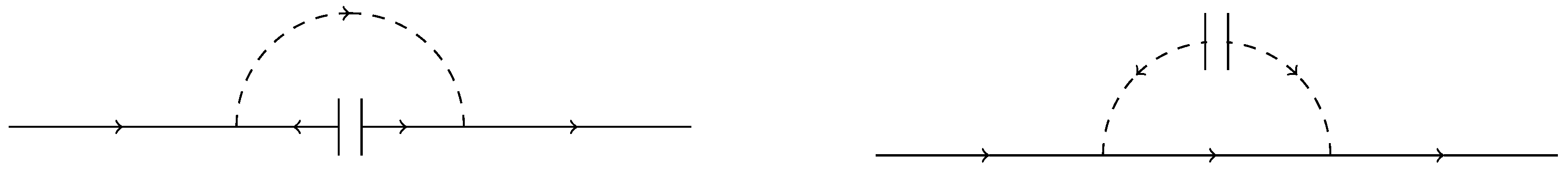
Let us begin by computing the leading contribution to in ; in other words, the terms that in the EFT power counting are of the order T. In Figure 2, we show the relevant diagrams. If we write as
and we use the notation of Equation (50), then the contribution from the diagrams in Figure 2 is
where is the temporal gluon propagator and is the first derivative over the temporal component of the spectral function of the temporal gluon propagator [16]. Our computation is performed in the Coulomb gauge.
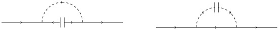
Figure 2.
Diagrams of contributions to at order T in . The computation is carried out on the Keldysh basis.
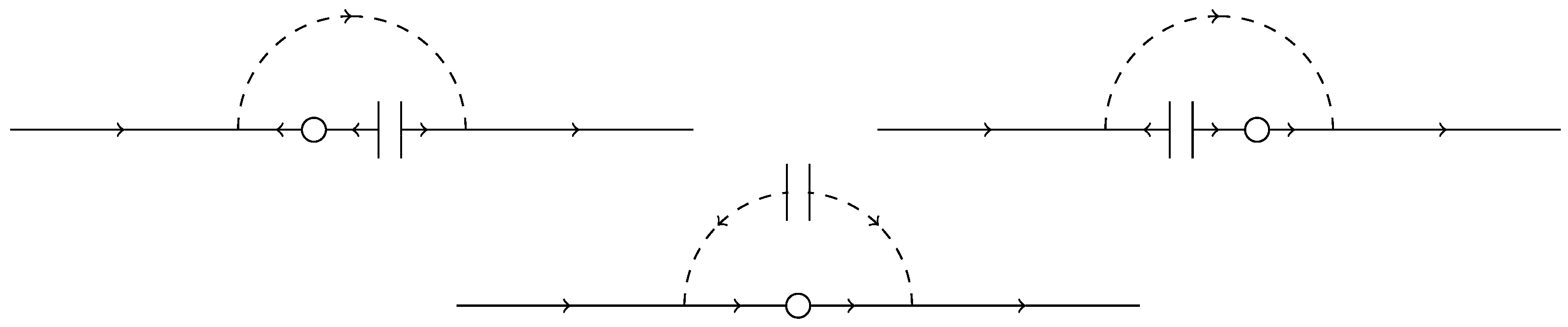
Next, let us discuss the possible corrections to and of the order . By symmetry arguments, there should not be any. However, let us check explicitly that this is the case. The relevant diagrams are shown in Figure 3. Each circled correction to the propagator introduces a factor , where is the spatial momentum of the temporal gluon. We can take out of the integrand, and since the medium does not have any preferred direction in space, the result of the integration can only be zero.
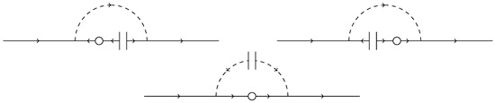
Figure 3.
Diagrams of contributions to at order in .
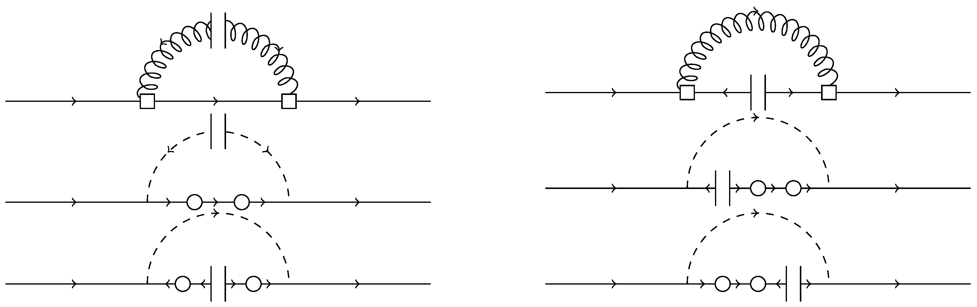
Regarding the diagrams contributing at the order , we can divide them into two classes: those that contribute to and , and those contributing to and . The first class is shown in Figure 4. They give the following contributions:
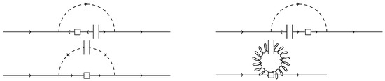
Figure 4.
Diagrams of contributions to and in .
Diagrams contributing to and are shown in Figure 5. They result in the following contributions:
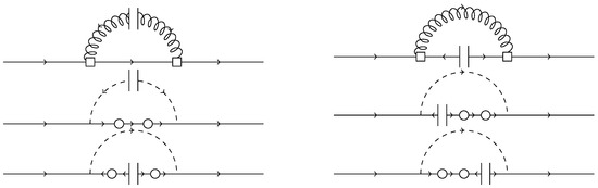
Figure 5.
Diagrams of contributions to and in .
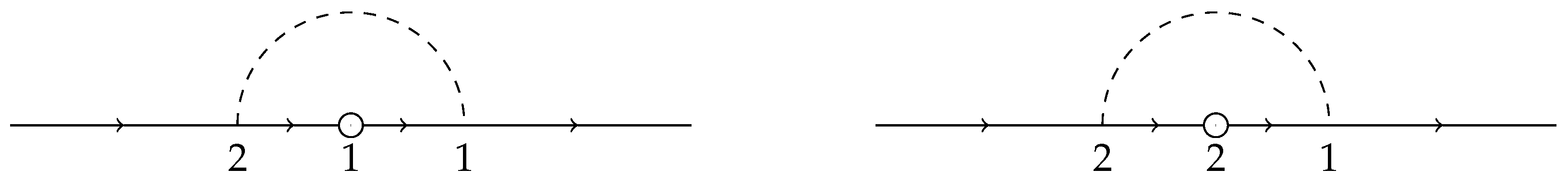
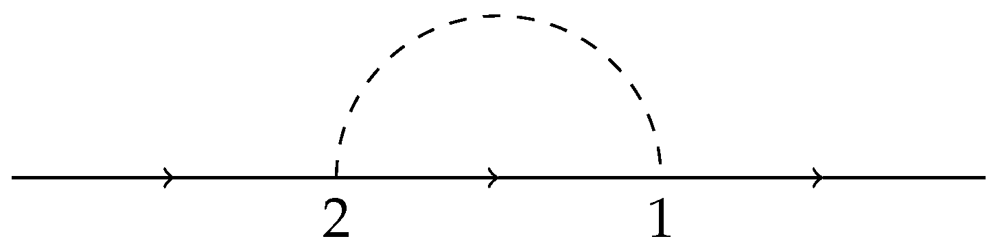
Let us now compute in in order to perform the matching. We are going to focus on the piece proportional to since, as we discussed previously, it is the only extra term needed to perform the matching. To obtain this, we need to go to the second order in the expansion shown in Equation (23). Moreover, we have to take from the Lagrangian the interaction similar to . Therefore, we need to focus on the diagram shown in Figure 6. Note that, for the computation of , we are using the basis instead of the Schwinger-Keldysh one. From this matching, we obtain
We can check that this result is compatible with the perturbative computation of in the Coulomb gauge [25,45,47]. Note that, in the limit, we can approximate by , as long as we are not using the unitary gauge. It is also important to take into account that we are enganging in a slight abuse of language by identifying the transport coefficient with the Wilson coefficient of LET. Strictly speaking, the Wilson coefficient only includes the contribution to from the scale we are integrating out, in this case T.
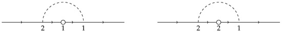
Figure 6.
Diagrams involved in the matching of .
With this, we have finished the matching to the order of interest. However, for the sake of cross-checking some of the relations we discussed in the previous section, we are going to discuss an alternative way to match the value of . This can be achieved looking at the diagram in Figure 7. However, now we have to take the third term in Equation (23) to get the contribution proportional to . Doing this, we can check that we obtain exactly the same value of . There is even a third way of computing which is to look at the terms in that function similarly to and subtract . However, we will not discuss further this way of achieving the matching of .
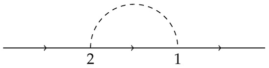
Figure 7.
An alternative diagram to consider in order to match .
Now we are ready to discuss how to derive a Fokker–Planck equation for heavy quarks in QCD including the effects of the scales T and . The first step has already been discussed. We match to LET to include the effect of the scale T in the Wilson coefficients. The second step is to compute and in LET, including the effects of the scale . Note, however, that the same symmetries and cancellations apply now, and, therefore, we only need to compute the contribution of the scale to . This can be obtained by computing the diagram in Figure 6, but now the loop has to be computed using the HTL gluon propagator. Proceeding in this way, we obtain the perturbative estimate of . This corresponds to Equation (60) but now using the two loop perturbative result for and the HTL approximation for [25,47].
6. Heavy Quarks with Momentum
In this section, we discuss the case of a heavy quark with a tri-momentum of order T. In this case, we will proceed as follows:
- As a starting point, we will use NRQCD Lagrangian.
- We will integrate out the scale T. After this, we will arrive again to LET. However, now the Wilson coefficients and the power counting will be slightly different, since p is now of the order T instead of as before.
- In this case, will have a more involved dependency with p. As a result, instead of a Fokker–Planck equation, we obtain an evolution similar to a Boltzmann equation.
Let us start looking at LET. The Lagrangian is again formed by combining Equations (25) and (28) in the same way as before. The main difference is the value of the Wilson coefficients.
Regarding and , it is easy to check that the results are exactly the same as in the case . The reason is that the diagrams that appear and carry out the respective matchings in (for ) and in NRQCD (for ) are the same at any order in the coupling constant, the only difference being the relative size of each term. However, the situation is different for ; the reason for this is that now this Wilson coefficient is, in general, a non-trivial function of f and p and we cannot assume a polynomial form like in Equation (54). However, we can assume that it is a polynomial in inverse powers of from the structure of NRQCD. Then, we can write
There are several constraints that can be imposed on . Equation (48) must be fulfilled, but now we need to take into account that we need to expand to the order desired since . This implies that
Additional constraints come from unitarity. We can repeat the arguments of Section 4 to arrive at
Imposing that , we deduce that
Starting from the previous equation and using the change of variables , we obtain the additional constraint
Using the previous equation and some trivial manipulations, we arrive at our final form of the evolution equation
As an illustration, let us discuss the perturbative matching. This can be carried out by looking at the diagrams in Figure 6 and Figure 7, but now taking into account that the expansion in Equation (23) cannot be achieved since . We obtain that
In fact, the last equation seems to be true at any perturbative order just because of the structure of NRQCD. We can see explicitly that the conditions in Equations (62) and (65) are fulfilled.
Finally, let us discuss the physical picture that the EFT treatment of the cases and provides when they are put together. If we start with a heavy quark at rest with the medium, it will start to gain momentum due to collisions. At this stage, the evolution of the system is given by a Boltzmann equation like Equation (66). This evolution is such that there is almost an equal probability to gain momentum than to lose it. Therefore, we will naturally arrive at a situation in which after some time. In this case, the evolution can already be described by a Langevin equation. As the momentum keeps increasing, the drag force starts to become important. Finally, we arrive to an equilibrium distribution in which momenta much larger than are very rare. Let us note that the arguments needed to arrive at these qualitative statements are valid, even if the medium is strongly coupled.
7. Discussion and Conclusions
In this manuscript, we have discussed an EFT approach to the derivation of the evolution of a heavy quark in a medium. Our main motivation was to pave the way for future developments in the study of quarkonium suppression. We would like to obtain a Lindblad equation for quarkonium without assuming a weakly coupled plasma and using the hierarchy of energy scales that appears in the problem. This has already been achieved in the case that the medium sees quarkonium as a small color dipole [10,11]. However, we would like to generalize to the case , as this would allow modeling more realistically excited states of bottomonium and charmonium at LHC energies. This is challenging because the EFT in which heavy quarkonium is best described is pNRQCD, and it is obtained after integrating out the scale . However, if , the matching between NRQCD and pNRQCD is modified by the medium. The appearance of an imaginary part of the potential indicates that the medium induces dissipative effects that cannot be encoded in an effective action; instead, we need an influence functional in which terms mixing the two branches of the Schwinger-Keldysh contour appear. Therefore, we need to modify pNRQCD to include this kind of term. The motivation of this manuscript was to study a simpler case in order to pave the way for this modification of pNRQCD in the future.
The simpler case we studied is a single heavy quark interacting with a medium. We achieved this following the EFT philosophy, in which each energy scale must be treated separately using a series of EFTs. We distinguished two cases: the case and the case . In both cases, we start with NRQCD; however, in the first case, we integrate out the scale as an intermediate step going from NRQCD to . Finally, we integrate the scale T in both cases to go to a new EFT that we named LET. The structure of this EFT is given by Equation (39), which is one of the main results of this manuscript. This formula combines the constraints of the Keldysh symmetry together with the special features of heavy particles in the dilute limit. Further constraints are provided by the fluctuation–dissipation theorem, which, together with the EFT power counting, leads to Equation (55) for and to Equation (66) for . This is the second main result from this manuscript: that Equations (55) and (66) can be obtained simply by symmetry and power counting arguments within the EFT approach. The physical picture is also quite transparent; a heavy quark with a momentum of the order T can be described by a Boltzmann equation and will slowly increase its momentum until we reach a moment in which the momentum is large enough so that a Langevin equation becomes valid.
Let us now discuss in more detail the relevance of the study presented in this manuscript in the context of quarkonium suppression. We have seen that the state of a heavy quark cannot be described by a single position x; instead, we need the position in the upper (lower) Schwinger-Keldysh branch , (). Note that is related to p by the Wigner transform. The increase of p we discussed below is seen in coordinate space as a narrowing of the coordinate or, put differently, the density matrix becoming almost diagonal in the coordinate basis. This behavior has also been observed in quarkonium [48,49]. One main difference between the case of quarkonium and that of a single heavy quark is that the number of coordinates needed to describe the system doubles. In quarkonium, we can talk about the center-of-mass coordinate, R, and the relative coordinate, r. However, in non-equilibrium situations, we need to consider the doubling of degrees of freedom, and then we have to take into account four coordinates, , , , and . A complete EFT treatment of quarkonium would identify all the possible scale hierarchies that can be constructed with these coordinates and that appear in the problem of quarkonium suppression. The case studied in this manuscript corresponds to a situation in which the quark and the antiquark are very far apart, and we have studied the cases and . In [10,11], the case studied corresponds to and . Perturbative studies have shown that the Lindblad equation that appears in the case naturally leads to a decrease of . This produces a change in the power counting that, among other things, makes the drag force not a perturbation (NLO corrections in that include the drag force were added in [50,51]). Regarding the relation between the scales , T and E, pNRQCD has been studied for all possible relations [7,8,9] but only taking into account the part analogous to in the notation of Equation (24). This is enough to discuss spectroscopy, but not to study the evolution of quarkonium inside a plasma. What is missing is the construction of the analogous to in pNRQCD, something that we hope this work has helped to develop.
Finally, let us discuss possible extensions of the present work in the context of heavy quark propagation itself. As in any EFT, an obvious improvement would be to compute higher order corrections in the expansion to improve our knowledge about the evolution of . Another possible direction is to relax the assumptions about the symmetries of the problem. For example, until now, we have assumed that both the medium and the distribution of heavy quarks are homogeneous in space and isotropic. It would be interesting to relax these conditions, as they are not completely fulfilled in heavy-ion collisions. Finally, the case is also interesting. In this case, we would be studying the case of a heavy quark that loses energy until it thermalizes with the medium.
Funding
The work of MAE was supported by the Maria de Maetzu excellence program under project CEX2019-000918-M, by the Spanish Research State Agency under project PID2019-105614GB-C21, and by the grant 2021-SGR-249 of Generalitat de Catalunya.
Data Availability Statement
No new data were created or analyzed in this study. Date sharing is not applicable to this article.
Acknowledgments
MAE would like to thank, for the careful reading of the first version of this manuscript and providing useful comments, Juan Torres-Rincon, Joan Soto, Nora Brambilla, and Antonio Vairo.
Conflicts of Interest
The author declares no conflict of interest.
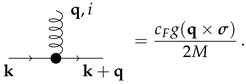
Appendix A. Feynmann Rules for NRQCDsh
The Lagrangian of the heavy quark sector of is
From now on, we will not write explicitly the sub-script in this section, as this quantity is conserved in all diagrams. The Feynmann rules for this theory are
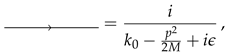
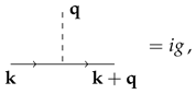
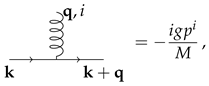
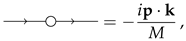
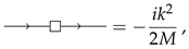
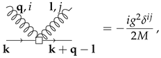
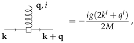
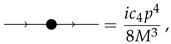 and, finally,
Appendix B. Gauge Invariance of
In this appendix, we are going to discuss the gauge invariance of Equation (28) in more detail. Let us focus on the simplest term that is already problematic
As we discussed, this term is only invariant under a restricted class of gauge transformations, those that transform in the same way in the fields in the two branches of the Schwinger-Keldysh contour. This term can be made gauge-invariant by including two extra Wilson lines.
where is a temporal Wilson line made of fields of type i. This term is gauge-invariant because fields of type 1 at are identical to fields of type 2 at . This is a consequence of the largest time equation [52] that implies that any correlator in which a quantum field (in the sense of Equation (34)) has the largest time argument is zero. In other words, quantum fields are zero at and so are their gauge transformations.
Let us now discuss the differences with [21] regarding an EFT for hydrodynamics. The fields of type 1 (or 2) were assumed to always appear in gauge-invariant conbinations thanks to the introduction of Stueckelberg-like fields [53]. However, this solution is not suitable in our case since the generalization of the Stueckelberg theory to non-Abelian symmetries is problematic [53]. Note that, in [21], they are dealing with a theory for the field in which only derivatives of this field can appear in the influence functional. This is not analog to our case, since the field appears without derivates in most of the terms we are interested in.
Now we can discuss the issue if the fields in and appearing in Equation (28) are of type 1 or 2. Let us first note that, if we impose that in the limit , then and the field inside need to be evaluated at time t. Regarding , there is only one possible combination because it can be verified that
where . Regarding B, it can be entered in the following combinations
Therefore, to be more precise, in Equation (28), we should change
into
Notes
| 1 | f is a function of and . However, we assume that f is a very smooth function in R when we look at distances of the order of . Therefore, we can consider that f does not depend on for the purposes of the matching and the study in this section. We also assume that the distribution is isotropic. |
| 2 | Propagators with a single arrow pointing to the right (left) are retarded (advanced). Propagators with two outgoing arrows and a capacitor symbol are symmetric. The rest of the symbols are defined in Appendix A. |
References
- Weinberg, S. Phenomenological Lagrangians. Phys. A 1979, 96, 327–340. [Google Scholar] [CrossRef]
- Caswell, W.E.; Lepage, G.P. Effective Lagrangians for Bound State Problems in QED, QCD, and Other Field Theories. Phys. Lett. B 1986, 167, 437–442. [Google Scholar] [CrossRef]
- Bodwin, G.T.; Braaten, E.; Lepage, G.P. Rigorous QCD analysis of inclusive annihilation and production of heavy quarkonium. Phys. Rev. D 1995, 51, 1125–1171, Erratum in Phys. Rev. D 1997, 55, 5853. [Google Scholar] [CrossRef] [PubMed]
- Pineda, A.; Soto, J. Effective field theory for ultrasoft momenta in NRQCD and NRQED. Nucl. Phys. B Proc. Suppl. 1998, 64, 428–432. [Google Scholar] [CrossRef]
- Brambilla, N.; Pineda, A.; Soto, J.; Vairo, A. Potential NRQCD: An Effective theory for heavy quarkonium. Nucl. Phys. B 2000, 566, 275. [Google Scholar] [CrossRef]
- Brambilla, N.; Pineda, A.; Soto, J.; Vairo, A. Effective Field Theories for Heavy Quarkonium. Rev. Mod. Phys. 2005, 77, 1423. [Google Scholar] [CrossRef]
- Escobedo, M.A.; Soto, J. Non-relativistic bound states at finite temperature (I): The Hydrogen atom. Phys. Rev. A 2008, 78, 032520. [Google Scholar] [CrossRef]
- Brambilla, N.; Ghiglieri, J.; Vairo, A.; Petreczky, P. Static quark-antiquark pairs at finite temperature. Phys. Rev. D 2008, 78, 014017. [Google Scholar] [CrossRef]
- Brambilla, N.; Escobedo, M.A.; Ghiglieri, J.; Soto, J.; Vairo, A. Heavy Quarkonium in a weakly-coupled quark-gluon plasma below the melting temperature. J. High Energy Phys. 2010, 9, 038. [Google Scholar] [CrossRef]
- Brambilla, N.; Escobedo, M.A.; Soto, J.; Vairo, A. Quarkonium suppression in heavy-ion collisions: An open quantum system approach. Phys. Rev. D 2017, 96, 034021. [Google Scholar] [CrossRef]
- Brambilla, N.; Escobedo, M.A.; Soto, J.; Vairo, A. Heavy quarkonium suppression in a fireball. Phys. Rev. D 2018, 97, 074009. [Google Scholar] [CrossRef]
- Yao, X.; Müller, B. Approach to equilibrium of quarkonium in quark-gluon plasma. Phys. Rev. C 2018, 97, 014908, Erratum in Phys. Rev. C 2018, 97, 049903. [Google Scholar] [CrossRef]
- Yao, X.; Mehen, T. Quarkonium in-medium transport equation derived from first principles. Phys. Rev. D 2019, 99, 096028. [Google Scholar] [CrossRef]
- Vaidya, V.; Yao, X. Transverse momentum broadening of a jet in quark-gluon plasma: An open quantum system EFT. J. High Energy Phys. 2020, 10, 024. [Google Scholar] [CrossRef]
- Vaidya, V. Effective Field Theory for jet substructure in heavy ion collisions. J. High Energy Phys. 2021, 11, 064. [Google Scholar] [CrossRef]
- Bellac, M.L. Thermal Field Theory; Cambridge Monographs on Mathematical Physics, Cambridge University Press: Cambridge, UK, 2011. [Google Scholar] [CrossRef]
- Breuer, H.P.; Petruccione, F. The Theory of Open Quantum Systems; Oxford University Press: Oxford, UK, 2007. [Google Scholar] [CrossRef]
- Feynman, R.P.; Vernon, F.L., Jr. The Theory of a general quantum system interacting with a linear dissipative system. Ann. Phys. 1963, 24, 118–173. [Google Scholar] [CrossRef]
- Baidya, A.; Jana, C.; Loganayagam, R.; Rudra, A. Renormalization in open quantum field theory. Part I. Scalar field theory. J. High Energy Phys. 2017, 11, 204. [Google Scholar] [CrossRef]
- Haehl, F.M.; Loganayagam, R.; Rangamani, M. Schwinger-Keldysh formalism. Part I: BRST symmetries and superspace. J. High Energy Phys. 2017, 06, 069. [Google Scholar] [CrossRef]
- Crossley, M.; Glorioso, P.; Liu, H. Effective field theory of dissipative fluids. J. High Energy Phys. 2017, 09, 095. [Google Scholar] [CrossRef]
- Jensen, K.; Pinzani-Fokeeva, N.; Yarom, A. Dissipative hydrodynamics in superspace. J. High Energy Phys. 2018, 09, 127. [Google Scholar] [CrossRef]
- Svetitsky, B. Diffusion of charmed quarks in the quark-gluon plasma. Phys. Rev. D 1988, 37, 2484–2491. [Google Scholar] [CrossRef] [PubMed]
- Torres-Rincon, J.M. Hadronic Transport Coefficients from Effective Field Theories. Ph.D. Thesis, Universidad Complutense de Madrid, Madrid, Spain, 2012. [Google Scholar] [CrossRef]
- Moore, G.D.; Teaney, D. How much do heavy quarks thermalize in a heavy ion collision? Phys. Rev. C 2005, 71, 064904. [Google Scholar] [CrossRef]
- van Hees, H.; Greco, V.; Rapp, R. Heavy-quark probes of the quark-gluon plasma at RHIC. Phys. Rev. C 2006, 73, 034913. [Google Scholar] [CrossRef]
- Rapp, R.; van Hees, H. Heavy Quark Diffusion as a Probe of the Quark-Gluon Plasma. arXiv 2008, arXiv:0803.0901. [Google Scholar]
- Akamatsu, Y.; Hatsuda, T.; Hirano, T. Heavy Quark Diffusion with Relativistic Langevin Dynamics in the Quark-Gluon Fluid. Phys. Rev. C 2009, 79, 054907. [Google Scholar] [CrossRef]
- Young, C.; Shuryak, E. Charmonium in strongly coupled quark-gluon plasma. Phys. Rev. C 2009, 79, 034907. [Google Scholar] [CrossRef]
- Bauer, C.W.; Fleming, S.; Pirjol, D.; Stewart, I.W. An Effective field theory for collinear and soft gluons: Heavy to light decays. Phys. Rev. D 2001, 63, 114020. [Google Scholar] [CrossRef]
- Bauer, C.W.; Pirjol, D.; Stewart, I.W. Soft collinear factorization in effective field theory. Phys. Rev. D 2002, 65, 054022. [Google Scholar] [CrossRef]
- Manuel, C.; Torres-Rincon, J.M. Chiral transport equation from the quantum Dirac Hamiltonian and the on-shell effective field theory. Phys. Rev. D 2014, 90, 076007. [Google Scholar] [CrossRef]
- Manuel, C.; Soto, J.; Stetina, S. On-shell effective field theory: A systematic tool to compute power corrections to the hard thermal loops. Phys. Rev. D 2016, 94, 025017, Erratum in Phys. Rev. D 2017, 96, 129901. [Google Scholar] [CrossRef]
- Brambilla, N.; Pineda, A.; Soto, J.; Vairo, A. The (m Lambda QCD)**1/2 scale in heavy quarkonium. Phys. Lett. B 2004, 580, 60–71. [Google Scholar] [CrossRef]
- Escobedo, M.A. Medium evolution of a static quark-antiquark pair in the large Nc limit. Phys. Rev. D 2021, 103, 034010. [Google Scholar] [CrossRef]
- Bu, Y.; Zhang, B. Schwinger-Keldysh effective action for a relativistic Brownian particle in the AdS/CFT correspondence. Phys. Rev. D 2021, 104, 086002. [Google Scholar] [CrossRef]
- Luke, M.E.; Manohar, A.V. Reparametrization invariance constraints on heavy particle effective field theories. Phys. Lett. B 1992, 286, 348–354. [Google Scholar] [CrossRef]
- Vasak, D.; Gyulassy, M.; Elze, H.T. Quantum Transport Theory for Abelian Plasmas. Annals Phys. 1987, 173, 462–492. [Google Scholar] [CrossRef]
- Keldysh, L.V. Diagram technique for nonequilibrium processes. Zh. Eksp. Teor. Fiz. 1964, 47, 1515–1527. [Google Scholar]
- Braaten, E.; Pisarski, R.D. Simple effective Lagrangian for hard thermal loops. Phys. Rev. D 1992, 45, R1827. [Google Scholar] [CrossRef] [PubMed]
- Chou, K.C.; Su, Z.B.; Hao, B.L.; Yu, L. Equilibrium and Nonequilibrium Formalisms Made Unified. Phys. Rept. 1985, 118, 1–131. [Google Scholar] [CrossRef]
- Greiner, C.; Leupold, S. Stochastic interpretation of Kadanoff-Baym equations and their relation to Langevin processes. Ann. Phys. 1998, 270, 328–390. [Google Scholar] [CrossRef]
- Baym, G.; Kadanoff, L.P. Conservation Laws and Correlation Functions. Phys. Rev. 1961, 124, 287–299. [Google Scholar] [CrossRef]
- Sheng, X.L.; Weickgenannt, N.; Speranza, E.; Rischke, D.H.; Wang, Q. From Kadanoff-Baym to Boltzmann equations for massive spin-1/2 fermions. Phys. Rev. D 2021, 104, 016029. [Google Scholar] [CrossRef]
- Casalderrey-Solana, J.; Teaney, D. Heavy quark diffusion in strongly coupled N = 4 Yang-Mills. Phys. Rev. D 2006, 74, 085012. [Google Scholar] [CrossRef]
- Ghiglieri, J.; Kurkela, A.; Strickland, M.; Vuorinen, A. Perturbative Thermal QCD: Formalism and Applications. Phys. Rept. 2020, 880, 1–73. [Google Scholar] [CrossRef]
- Caron-Huot, S.; Laine, M.; Moore, G.D. A Way to estimate the heavy quark thermalization rate from the lattice. J. High Energy Phys. 2009, 04, 053. [Google Scholar] [CrossRef]
- Blaizot, J.P.; Escobedo, M.A. Quantum and classical dynamics of heavy quarks in a quark-gluon plasma. J. High Energy Phys. 2018, 06, 034. [Google Scholar] [CrossRef]
- Delorme, S. Theoretical Description of Quarkonium Dynamics in the Quark Gluon Plasma with a Quantum Master Equation Approach. Ph.D. Thesis, Laboratoire de Physique Subatomique et des Technologies Associées, France, IMT Atlantique, Nantes, France, 2021. [Google Scholar]
- Brambilla, N.; Escobedo, M.A.; Islam, A.; Strickland, M.; Tiwari, A.; Vairo, A.; Vander Griend, P. Heavy quarkonium dynamics at next-to-leading order in the binding energy over temperature. J. High Energy Phys. 2022, 08, 303. [Google Scholar] [CrossRef]
- Brambilla, N.; Escobedo, M.A.; Islam, A.; Strickland, M.; Tiwari, A.; Vairo, A.; Vander Griend, P. Regeneration of bottomonia in an open quantum systems approach. Phys. Rev. D 2023, 108, L011502. [Google Scholar] [CrossRef]
- Veltman, M.J.G. Unitarity and causality in a renormalizable field theory with unstable particles. Physica 1963, 29, 186–207. [Google Scholar] [CrossRef]
- Ruegg, H.; Ruiz-Altaba, M. The Stueckelberg field. Int. J. Mod. Phys. A 2004, 19, 3265–3348. [Google Scholar] [CrossRef]

Disclaimer/Publisher’s Note: The statements, opinions and data contained in all publications are solely those of the individual author(s) and contributor(s) and not of MDPI and/or the editor(s). MDPI and/or the editor(s) disclaim responsibility for any injury to people or property resulting from any ideas, methods, instructions or products referred to in the content. |
© 2024 by the author. Licensee MDPI, Basel, Switzerland. This article is an open access article distributed under the terms and conditions of the Creative Commons Attribution (CC BY) license (https://creativecommons.org/licenses/by/4.0/).