1. Introduction
The Standard Model (SM) of electroweak and strong interactions provides an extremely successful description of particle physics up to the (roughly) TeV scale. However, there are reasons to go beyond the SM (for an introduction see [
1]). Interestingly, a plethora of scalar degrees of freedom can appear into the effective theories describing the low-energy regime of these extensions of the SM.
One remarkable example is given by string theory (see, for example, [
2]), where gauge neutral scalar fields with perturbatively flat potential (
i.e., moduli fields) are present. These moduli can be coupled to matter and they can control the value of the fundamental “constants”. Therefore, in order to construct a realistic string model, the stabilization of the moduli is, typically, a crucial step. In other words, if we stabilize (
i.e., we give a large mass to) the moduli we can obtain a model such that (1) the range of the modulus-mediated interaction is short and (2) the fundamental “constants” are really fixed. In a realistic scenario, the conditions (1) and (2) are certainly welcome and many efforts have been dedicated to moduli stabilization (see for example [
3] and related references).
This review will discuss the so-called “chameleon” mechanism. It can be considered a stabilization mechanism, but it is very peculiar, because it is related to the large density of the local environment. The chameleon mechanism is also a screening mechanism: the deviations from standard General Relativity (GR) are suppressed locally exploiting the large (Large with respect to the cosmological value) density of the local environment. To date, three screening mechanisms turned out to be successful:
The chameleon mechanism [
4,
5], where a field (typically scalar) has a mass that depends on the matter density of the environment: the larger is the matter density, the larger is the mass of the chameleon. On cosmological distances, where the matter density is small, the chameleon is ultralight and, hence, it can play the role of a sort of quintessence field. Interestingly, in [
6,
7,
8,
9,
10] a chameleonic model that keeps under control the cosmological constant without fine-tuning of the parameters and including all quantum contributions has been discussed.
The Vainshtein mechanism [
11] takes advantage of the non-linearities sourced by the self-coupling of a scalar field.
The symmetron mechanism [
12,
13,
14] where fifth forces are screened through the restoration of a symmetry at high-density.
Let us discuss the first mechanism. Two issues are particularly relevant. On the one hand, stronger theoretical grounds supporting chameleonic theories are welcome (many efforts have been dedicated to this topic—see for example [
6,
9,
15,
16,
17,
18,
19]), on the other hand, experimental signatures of chameleons.
Let us further elaborate the point we mentioned last. At the moment, it is not known whether chameleon fields are present in Nature or not. The search for chameleon fields has been performed in various ways. Let us summarize some of them:
- (1)
In the Laboratory. In this case we mention three experiments: the E
t-Wash experiment [
20], the CHASE experiment [
21], the ADMX experiment (Axion Dark Matter eXperiment) [
22]. The first one is designed to investigate potential deviations from the inverse-square law of gravity on length scales larger than (roughly) 50 μm. Let us now briefly touch upon the remaining two experiments. CHASE and ADMX experiments are based on the potential presence of a coupling between the chameleon field and the
term of photons. This coupling, in the presence of a magnetic field, can lead to oscillations photons-chameleons that might be detected by CHASE and ADMX.
- (2)
Astrophysically. As already discussed in [
23], PLANCK data put tight constraints on
(at
C.L.) which parametrizes the non-minimal coupling chameleon-matter (in GR we have
). PLANCK data are not the only source of astrophysical/cosmological constraints. For example, the photon-chameleon mixing mentioned above can occur inside the Sun [
24] and this might explain the solar corona problem. The same mixing photons-chameleons can occur inside the magnetic field of the Coma cluster: in this case a chameleonic Sunyaev-Zeldovich (CSZ) effect has been predicted. In other words, the CSZ effect is a reduction of the overall photon intensity due to the conversion photon-chameleon inside the magnetic field. It is similar to the standard SZ effect due to the interaction photons-electrons. However, there is a difference: the standard SZ effect decreases rapidly towards the edge of the cluster where the number density of the electrons is small while, by contrast, the CSZ effect depends on the ratio of the magnetic field to the electron density and, therefore, it might be the origin of the greater than expected SZ signal detected at large radii [
25,
26]. Moreover, chameleons affect the internal dynamics and stellar evolution in dwarf galaxies in regions with a sufficiently small density (see [
27] and references therein). For a discussion of the link between chameleon fields and helioseismology see [
28].
- (3)
Performing Tests of Gravity in Space. Interestingly, small bodies that are screened in the laboratory can be unscreened in space, where the matter density is much smaller. Hence, chameleons can produce violations of the weak equivalence principle (WEP) in orbit with
, in conflict with the corresponding laboratory constraints. Analogously,
(1) deviations from the value of
measured on Earth are expected in the theory. These properties of chameleons lead to interesting predictions for future satellite experiments designed to test gravity in space such as MicroSCOPE (
http://microscope.onera.fr/) and STE-QUEST (
http://sci.esa.int/science-e/www/area/index.cfm?fareaid=127.)
Interestingly, chameleon fields are relevant not only for phenomenological reasons, but also for theoretical ones. For example they are a useful guideline towards the construction of a quantum theory of gravitation. Indeed, in [
10] a Chameleonic Equivalence Principle (CEP) has been formulated as a consequence of the chameleon mechanism. The CEP establishes an equivalence between a conformal anomaly and the quantum gravitational field. This principle is formulated in the so-called Modified Fujii’s Model (MFM) which has been exploited in [
6] to solve the Cosmological Constant (CC) problem. Let us further discuss this issue. In the E-frame of the MFM a chameleonic dilaton
σ is parametrizing the scale invariance of the model. Locally, in the UV (ultraviolet), scale invariance is abundantly broken, particle masses are large, the vacuum energy is large. On the contrary, globally, in the IR region, particles are very light, the renormalized vacuum energy is small and scale invariance is basically restored. The non-linear nature of the chameleonic theory is crucial to keep under control the CC. The reader is referred to [
6] for more details. It is common knowledge that the CC problem is really acute only in the quantum gravity regime and, hence, the CEP is a step beyond the (basically) semi-classical analysis of [
6]. Another theoretical reason to consider chameleon fields is that they can describe (in the MFM) the collapse of the wave function in quantum mechanics [
10] and the CEP is telling us that the collapse is a quantum gravity effect. For example, let us consider a diffraction experiment with electrons (forming a plane wave) scattered through a circular hole. The system is axially-symmetric. When we perform a quantum measurement, namely, when the electrons enter into the screen, there is a shift in the matter density of the environment, the chameleon jumps to another ground state and the harmonic approximation is broken during the jump. Therefore, the non-linear nature of the theory breaks the superposition principle for a short time. The expected diffraction pattern will respect the circular symmetry (
i.e., it corresponds to a set of degenerate states), but the single electron on the screen will break the symmetry. Where does this symmetry breaking come from? The chameleonic lagrangian is rotationally symmetric but the vacuum is not. This is the condition to obtain spontaneous symmetry breaking. This is exactly the path followed in [
10]: spontaneous breakdown of rotational symmetry is useful to justify the diffraction pattern on the screen. For further details about the chameleon-induced collapse of the wave function, the reader is referred to [
10,
29].
As far as the organization of this review is concerned, in
Section 2 we will present the standard chameleonic scenario with a discussion of the conformal transformation and of the thin-shell mechanism. In
Section 3 we will further explore the connection between chameleon fields and alternative theories of gravitation. In particular we will analyze
theories and also the MFM. In the final paragraph we will briefly summarize some concluding remarks.
As already mentioned above, this is a short review about chameleons. For further details on the subject the reader is referred to [
27,
30,
31,
32] for reviews and to [
33] for a recent summary of some experimental constraints. For a discussion of the stability issue in cosmology the reader is referred to [
34].
As far as our notation is concerned, we will follow the standard notations of the chameleonic literature and we will call the E-frame metric, while the J-frame metric will be called or, when we consider different sets of matter particles, . The only exception will be in the last section where a different notation will be exploited (and explained).
2. Standard Chameleonic Theories
A chameleon scalar field [
4,
5] is a scalar field coupled to matter (including the baryonic one) with gravitational strength (or even higher [
35]) and with a mass dependent on the density of the environment. Before the proposal of [
4,
5], a discussion of these ideas had been given in theories with time-varying alpha in [
36,
37]. Here we are going to consider only scalar fields, however also chameleonic vector fields have been discussed in the literature [
38].
The name “chameleon” is due to the peculiar environment-dependent mass of the field. For example, on very large (
i.e., cosmological) length scales, we know that the matter density is extremely small and, in this case, the chameleon mechanism is (almost) not operative. Hence the mass of the chameleon can be of the order of the Hubble constant and the field can roll down the potential on cosmological time scales (for a discussion of ultralight scalar fields in connection to the accelerated expansion of a low redshift Universe see [
39]). The careful reader may be worried by this set up, because, for phenomenological reasons, in general it’s not possible to introduce in a model a very light scalar field with a generic coupling with matter. However, this situation is modified if we consider small length scales, for example, “this room”. In this second case, indeed, the density is higher, the chameleon mechanism is operative and the field acquires a mass that is large enough to satisfy all experimental bounds on deviations from general relativity (GR). The chameleon mechanism is a screening mechanism.
To see how this works, let us consider the following scalar-tensor (ST) theory in the E-frame (see for example [
40]):
where
ϕ is the chameleon scalar field,
β is a real constant that will be discussed later,
is the Planck mass and
is the scalar potential. Fermion (matter) fields, denoted by
, couple conformally to the chameleon through the
dependence of the matter lagrangian
.
A crucial point about the chameleon field is realizing that the dynamic behavior of the field is not determined only by a potential but it is governed by an effective potential,
, which depends explicitly on
(energy density of non-relativistic matter, conserved with respect to the Einstein frame metric):
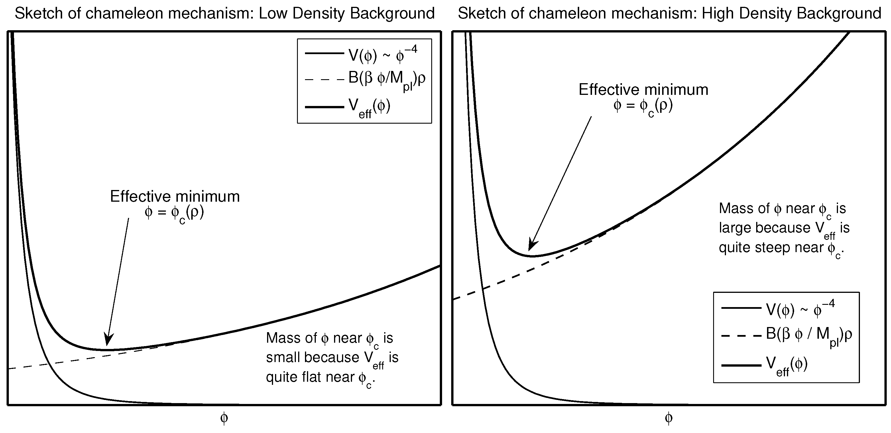
A typical example of chameleonic scenario is given by a run-away “bare” potential
and by a matter branch where
increases with
ϕ. In this way, a “competition” between the two branches of the curve is created and, therefore, the chameleonic environment-dependent mass is obtained. The minimum of the effective potential and the mass of the field in the minimum,
, both depend on
(see
Figure 1) Actually, a run-away bare potential is not strictly necessary if our intention is to construct a chameleon field.
Figure 1.
Chameleon mechanism for a runaway potential:
. The matter density is small in the left plot and it’s large in the right plot (see [
30]). The mass of the chameleon is an increasing function of the background matter density. These plots can be found in [
30]. (Reprinted figures with permission from David F. Mota and Douglas J. Shaw.
Phys. Rev. 2007,
D75, 063501. Copyright (2007) by the American Physical Society. Source:
http://journals.aps.org/prd/abstract/10.1103/PhysRevD.75.063501)
This chameleon mechanism is often related in macroscopic bodies with the so-called “thin-shell”. A body has a thin-shell if ϕ is approximately constant everywhere inside the body but in a small region (the thin-shell) near the surface of the body, where large () variations of ϕ can occur. Inside a body with a thin-shell vanishes everywhere apart from a thin superficial layer. The force mediated by ϕ is proportional to , consequently, only the thin-shell feels and contributes to the chameleon-mediated “fifth force”.
Needless to say, experimental bounds on the coupling between the chameleon and matter must be taken into account. For this purpose, the thin-shell effect plays a crucial role. For example: in the solar system, the standard chameleon field can be very light and, hence, it can mediate a long-range force whose phenomenological consequences might be unacceptable because the limits on such forces are very tight. However, since the chameleon is coupled only to a small fraction of the matter in large bodies (
i.e., that fraction in the thin-shell), the chameleon force between the Sun and the planets is very weak. We infer that the “dangerous” bounds on long-range forces are faced [
4,
5]. As we will see, the thin-shell mechanism is related to the non-linear nature of the chameleon theories.
2.1. The Typical Set Up
In the original proposal [
4,
5], the chameleon mechanism is obtained by giving the scalar field a potential
and a coupling to matter described by a function
; where
ρ is the local matter density and
B is a function to be specified later. The potential and the coupling to matter create an effective potential:
. The values
ϕ takes at the minima of this effective potential are environment-dependent.
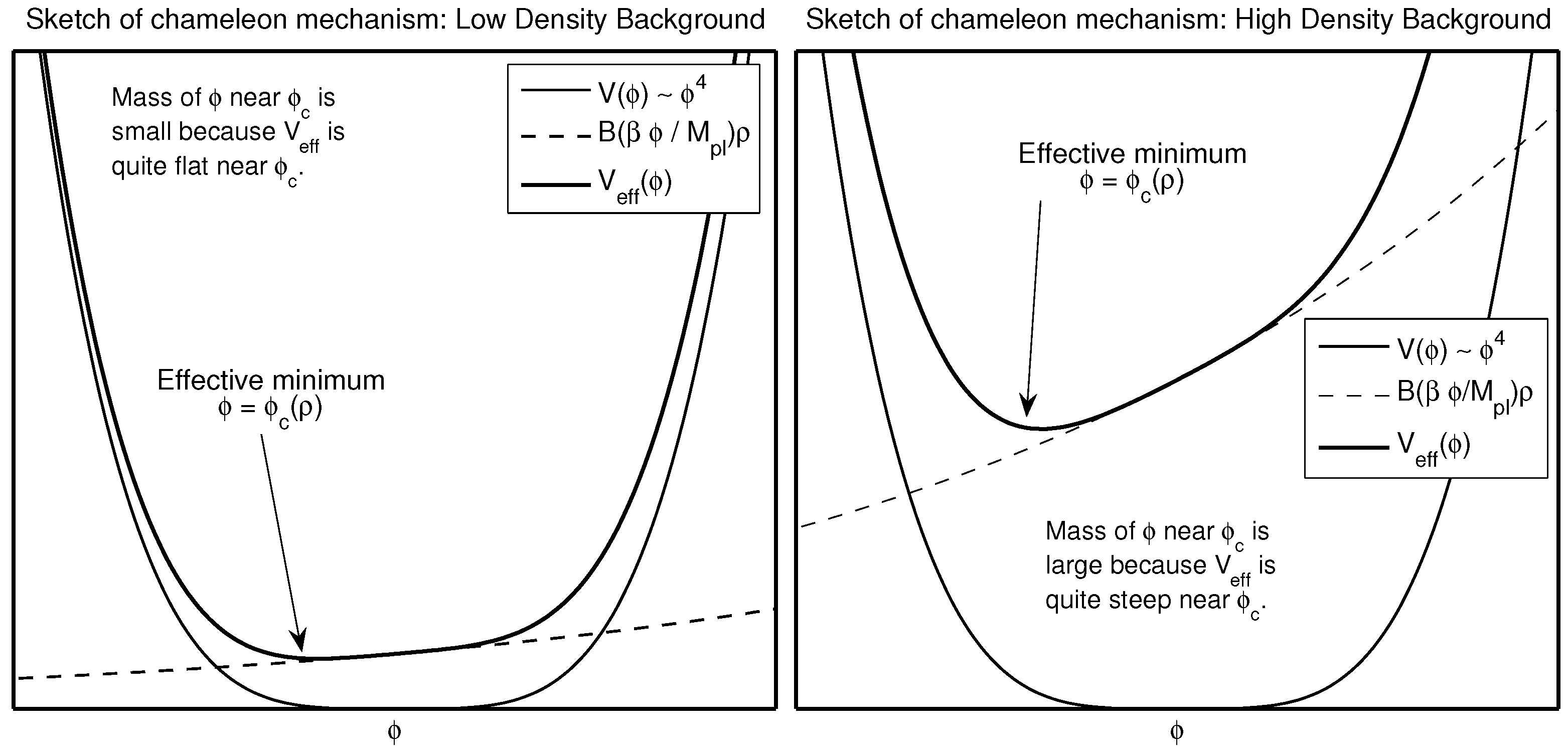
If is a critical point of the effective potential, i.e., , then the effective “mass” () of the field about will be obtained evaluating the second derivative of the effective potential (). If is neither constant, linear nor quadratic in ϕ then , and hence the mass , will depend on . Since depends on the matter density, also the effective mass will be environment-dependent. A potential with these properties will lead us to non-linear field equations for ϕ.
For a scalar field theory to be chameleonic, the effective mass of the scalar must be an increasing function of the matter density and, therefore,
. As already mentioned above, it is not necessary for either
or
to have any minima themselves if our intention is to construct a minimum in the effective potential. The chameleon mechanism is summarized in
Figure 1 and
Figure 2.
Figure 2.
Chameleon mechanism for a potential with a minimum at
:
. The left plot corresponds to small matter density and the plot to the right corresponds to large matter density (see [
30]). Once again, the mass of the chameleon is growing with the matter density. These plots can be found in [
30]. (Reprinted figures with permission from David F. Mota and Douglas J. Shaw.
Phys. Rev. 2007,
D75, 063501. Copyright (2007) by the American Physical Society. Source:
http://journals.aps.org/prd/abstract/10.1103/PhysRevD.75.063501)
These plots require some additional remarks. In
Figure 1 we have a run-away potential, but
does have a minimum due to the presence of the matter branch and the value of
ϕ in that minimum is density dependent. In
Figure 2 the potential is
and so it does have a minimum at
(it is not run-away), however, the minimum of the effective potential does not coincide with that of
V because the chameleonic coupling to matter creates a shift of the ground state.
Typically when a scalar field
ϕ is coupled to matter, one of the effects of the coupling is a non-trivial
ϕ-dependence of the mass
m of the matter particle (
i.e., the coupling is encoded into a mass-varying term, no matter whether we consider this coupling as a classical one or as a result of quantum corrections). The
ϕ-dependence of
m can be written as
where
is the Planck mass and
is some constant with units of mass whose definition will depend on the choice of the function
.
β defines the strength of the coupling of
ϕ to matter. In general, a consequence of a
ϕ-dependent mass of a matter particle is a
ϕ-dependence of the rest-mass density of this particle:
The coupling of
ϕ to the local energy density of this particle species is given by
which is:
where
and
.
If we linearize
we find:
This truncation is acceptable granted that .
If , we can use the freedom in the definition of β to set and, in this case, β parametrizes the strength of the chameleon-to-matter coupling.
For example: a particular choice for
B that has been discussed in the literature ([
4,
5,
41]) is
for some
k. It follows that
, and so we choose
which ensures
,
.
2.2. One Possible Lagrangian
The standard Einstein-Hilbert action is given by
Let us introduce a scalar field
ϕ with potential
and action
We now define
and we introduce a set of matter fields
with action
which are coupled to
ϕ by the conformal transformation that, for example, we write as:
where
are dimensionless coupling constants, in principle one for each matter species (
i.e., multi-metric theory).
The total action which takes into account gravity,
ϕ and matter is thus written as Equation (
1), namely:
Variation with respect to
ϕ allows us to obtain the equation of motion for
ϕ. Following [
31] we write:
where on the first step we exploited the symmetry of the metric to get
.
On the second step we used the commutativity of differentiation with variation to obtain . On the third step, an integration by parts has been performed by applying the divergence theorem to and assuming that or at spacetime infinity or boundaries.
From
we obtain the field equation:
2.3. Matter Energy Density
In this subsection, following [
31], we will further analyze the matter energy density. We will fix
i and we will write
instead of
.
2.3.1. Jordan Frame
If we assume that the matter fields
do not interact with each other, each energy-momentum tensor
is conserved in the Jordan frame. Namely,
Let us assume the matter to be a perfect isentropic fluid with
. Then
2.3.2. Einstein Frame
Let us impose, without loss of generality, a Friedmann-Lemaître-Robertson-Walker (FLRW) background metric. The energy density ρ in the Einstein frame (the frame corresponding to ) is conformally related to and it satisfies the standard continuity equation .
Now we collect some useful formulas:
Let us compute the Christoffel symbols
(see [
31]) and let us use them to expand the conservation Equation (
10) with index
. When we differentiate we keep
ϕ fixed and we vary the scale factor
a:
Thus, multiplying by
:
In other words, in the Einstein frame, the quantity
is the energy density of matter, because it satisfies the continuity equation
.
The Einstein-frame energy density for each species
i is obtained restoring the
i subscripts and exploiting Equation (
11):
2.4. The Equation of Motion and the Potential
If we substitute Equation (
16) into Equation (
9), we obtain an equation of motion with an explicit
ϕ-dependence:
We infer that the dynamical behaviour of
ϕ is summarized by an effective potential
Then the chameleon equation of motion in the Einstein frame is simply
We can also write the equations in a slightly more general way:
The Lagrangian Equation (
1) should not be viewed as specifying the only way in which
ϕ can be coupled to matter. However, despite the fact that many different Lagrangians are possible, it is almost always the case that the field equation for
ϕ takes a form very similar to the one given above.
Remarkably, highly non-linear self-interaction potentials are necessarily present for the chameleon. The non-linear nature of the theory is a major obstacle if our intention is to obtain analytical solutions of the field equations and this problem is particularly acute with highly inhomogeneous matter density. A linear approximation may lead us to wrong conclusions about fifth-force experiments. When the non-linearities are properly taken into account, the chameleon mechanism becomes much stronger [
30,
31,
35] and this effect gives us the chance to construct models with light cosmological scalars coupled to matter much
more strongly than gravity (
).
To proceed further, we discuss some examples of self-interaction potentials that have been considered in the literature. Needless to say,
V is non-linear and non-quadratic. One example is given by the Ratra-Peebles potential,
, where
M is some mass scale and
; chameleon fields have also been studied in the context of
(see [
42]). Let us consider this potential:
where
n can be positive or negative and
. If
then we can scale
M so that
. When
,
M drops out and we have a
theory. When
this is just the Ratra-Peebles potential. When
, our choice of potential comes from an expansion, for small
, of another potential
where
f is some function. We could then write:
where
is some mass-scale. We define
M so that the second term on the right hand side of the above expression reads
. The first term on the right hand then plays the role of a CC
. If
and
are
, then the typical ansatz in the chameleonic literature is
. In other words, the CC scale is inserted by-hand (as already mentioned above this ansatz is not present in [
6] where no fine-tuning has been introduced in the model).
Consequently, we are led to the following field equations:
In order to render the chameleon mechanism operative, the potential gradient term and the matter coupling term must have opposite signs. It is usually the case that and . If we must therefore have . In theories with we must have and where p is a positive integer. Another condition that must be satisfied is that the mass squared of the chameleon must be positive and ϕ-dependent. These conditions mean that we must exclude the region . Interestingly, for , or the field equations would be linear.
2.5. The Thin-Shell Effect
In this (sub)section, following [
30], we will analyze the chameleonic field in the presence of a single body and we will discuss the solutions to Equation (
23) in three different regimes that will be quantitatively defined later, namely:
Let us consider a spherically symmetric object with uniform density
and radius
R in a background with uniform density
. We will work with a Minkowskian (at leading order) spacetime. Under these assumptions
where
;
. Inside the body (
) we assume spherical symmetry and, therefore,
ϕ obeys:
Outside the body
we have:
The right hand side of Equation (
24) vanishes in the minimum
inside the body, namely when
where
Similarly, the right hand side of Equation (
25) vanishes in the minimum of
outside the body, namely when
where
For large
r we must have
. The effective mass is given by:
We define
and
. We shall see below that the larger the quantity
gets, the more likely it is that a body will have a thin-shell. Throughout this section we will require these boundary conditions:
2.5.1. Linear Regime
We assume that it is a valid approximation to linearize the equations of motion for
ϕ about the value of
ϕ in the far background,
. The linear approximation is valid granted that certain conditions are satisfied. We will summarize these conditions later in this section. We write
and the linearized field equations are:
where
is the Heaviside function:
,
, and
,
. This linearization of the potential is acceptable granted that
and this gives
. Moreover, for this linearization to remain valid as
, we need
, which implies that
The solution to the field equations outside the body (
) is
where we defined
, while inside the body (
)
is given by
The largest value of
occurs at
and hence
is required for an acceptable linear approximation. This requirement is equivalent to
where “∼” means “asymptotically in the limit
”. As we can see from this last formula, if we consider the typical situation where
, then for theories with
, the lower the density of the background gets, the better the linear approximation will be (because
will be larger). On the contrary, when
the opposite is true.
2.5.2. Pseudo-Linear Regime
We now assume the existence of (at least) one self-consistent linearization of the field equations about every point (we will define these existence conditions later). We do not require the validity of this linearization everywhere. Instead we construct two linearizations of the field equations: the inner and the outer approximations to ϕ.
The inner approximation is an asymptotic approximation to the chameleon that is valid, on the one hand, inside an isolated body and, on the other hand, near the surface of that body. In general, the inner approximation will not be valid anymore far from the body ().
The second linearization, the outer approximation, is an asymptotic approximation to ϕ that is valid for large values of r, but, in general, not for . We require that it remains valid as .
The boundary conditions already mentioned above are:
We cannot apply the boundary condition to the outer-approximation. Similarly the boundary condition will be applicable to the outer-approximation but not to the inner one.
It is not possible to apply all the boundary conditions to both approximations and, consequently, there will be undefined constants of integration. However, these constants can be evaluated if we find an intermediate range of values of r ( say) where the inner and the outer approximations are both valid.
As pointed out in [
30] and references therein, asymptotic expansions are locally unique. Therefore, if both the outer and inner approximations are simultaneously valid in some intermediate region, then they must be equal to each other in that region.
Inner Approximation
Inside the body,
, the chameleon satisfies:
The inner approximation is defined by the assumption
We see that the above assumption is equivalent to:
We define the inner approximation by solving Equation (
28) for
ϕ as an asymptotic expansion in the small parameter
. It is noteworthy that
.
Whenever the inner approximation is valid we have:
for
with the order
δ term given by
is an undefined constant of integration to be determined by matching the inner approximation to the outer one. In order to guarantee the validity of the inner approximation inside the body we need:
Outside the body,
,
ϕ satisfies:
where the
ρ-matter contribution can be safely neglected because we are considering the solution close to the body. Whenever
, the above equation can be solved in the inner approximation (for an explicit expression of
for
see [
30]):
for
.
Hence, the inner approximation will be valid simultaneously inside and outside the body granted that
In general, this requirement will hold only for
r smaller than some finite value of
r (
).
Outer Approximation
When
r is very large, the presence of the body should induce only a small perturbation on
ϕ. If we assume that
for
, then the outer approximation is defined by the assumption
We infer that:
where
is the mass of the chameleon in the background. The assumption
is basically the same assumption considered in the linear approximation, with the difference that, in the pseudo-linear case, it is not required to hold up to
but only for
, where
is any value of
r smaller than
. In other words, some intermediate region where both (the inner and the outer) approximations are simultaneously valid is necessary.
Outside of the body
ϕ satisfies:
where the
ρ-matter contribution cannot be neglected anymore. In order to guarantee a valid outer approximation when
, it is necessary that
Solving for
ϕ in the outer approximation, we find
where:
χ is an unknown constant of integration that will be determined through the matching procedure.
Matching Procedure
Let us suppose that an intermediate region
exists where the inner and outer approximations are both valid (we will discuss the existence conditions of this open set below). In other words, an open set about some point
where both approximations are valid is required. We must also impose the validity of the inner approximation for all
and of the outer approximation for all
. In the intermediate region the uniqueness of the asymptotic expansion implies
and
A can be evaluated from this last formula and the result is:
Now that χ and have been determined, we will evaluate the existence conditions of an intermediate region.
2.5.3. Non-Linear Regime Close to the Body
If our intention is to analyze the evolution of
ϕ in the thin-shell, the curvature of the surface of the body can be neglected, because the thickness of the shell
is much smaller than
R. Consequently, we treat the surface of the body as a flat surface, with outward normal in the direction of the positive
x-axis. The surface of the body is by definition at
(
i.e.,
). Naturally, we are interested in physics over length-scales much smaller than the size of the body, because the shell is much thinner than the length scale of the body. Hence, we can exploit the approximation that the body extends to infinity along the
y and
z axes and also along the negative
x axis. With these assumptions,
ϕ satisfies
Our boundary conditions (BCs) are
and
as
. With these BCs, the first integral of the above equation is:
Outside of the body, we assume (1)
as
; and (2) a background with density
. If
is large enough, we can safely assume
then we can ignore the curvature of the surface of the body and, in
, we have:
Our assumption that
then requires that:
Near the surface of the body, we expect
granted that the pseudo-linear approximation breaks down and that the body has a thin-shell. Hence, whenever
, we have
and
. The above condition will therefore be satisfied provided that
; this is generally a weaker condition than the thin-shell conditions. On the surface, at
,
ϕ and
must be both continuous. If we impose the continuity condition of
at the surface, we infer [
30]:
As already mentioned above,
implies the existence of a thin-shell (
i.e.,
). Let us prove this statement. Near the surface of the body, almost all variation in
ϕ are expected to take place in a shell of thickness
. We define
by:
is then, approximately, the length scale over which any variation in
ϕ dies off. It follows that
. In order to (A) render this shell thin and (B) safely ignore the curvature of the surface of the body, we need
or equivalently
. If we assume
we can write [
30]:
and so
follows from
, and
.
will be automatically satisfied whenever the thin-shell conditions hold.
Whenever
, Equation (
36) will be well-approximated by
near
. If we solve this formula with the boundary conditions mentioned above, namely
and
as
, we have
Hence, if is large enough, then (and therefore also ϕ) will be independent of and consequently also of and β at leading order. We further elaborate on this point in the (sub)section below.
Summarizing, (1) the presence of a thin-shell is related to non-linear effects that are non-negligible near the surface of the body; (2) a thin-shell exists whenever is large enough.
2.5.4. Non-Linear Regime Far from the Body
Interestingly, even if
is large enough, non-linear effects should not be important far from the surface of the body. Indeed, for large
r,
ϕ should have a functional form similar to that found in the pseudo-linear approximation. We will consider here only run-away potentials (
) and we refer the reader to [
30] for a more complete discussion.
Away from the surface of the body we expect that non-linear effects will be negligible and as
we will have:
for some constant
where
and
are the values of the chameleon and its mass in the background. In
theories the potential is singular and we have
outside the body. The minimum value of
outside the body occurs at
and hence
Typically,
and therefore
This upper bound on
defines a critical form for the field outside the body:
No matter what occurs inside the body, we must have
outside the body as
. Ignoring non-linear effects,
is satisfied by all bodies that satisfy the conditions for the pseudo-linear approximation, but would be violated, in the absence of non-linear effects, by those that satisfy the thin-shell conditions. We must therefore conclude that non-linear effects near the surface of a body with thin-shell ensure
is always satisfied as
. Furthermore, if
then
and it follows from
Section 2.5.2 that the pseudo-linear approximation is valid for all
r, which further implies that the body cannot have a thin-shell. We are therefore justified in using
to approximate the far field of a body with a thin-shell.
There are a number of consequences of the existence of a critical form for ϕ when . In particular, no matter how massive our central body is, no matter how strongly it is coupled to the chameleon, the perturbation it produces in ϕ for takes a universal value whenever the thin-shell conditions are valid.
Remarkably, the far field is found to be independent of the coupling, β, of the chameleon to the isolated body. The β independence is a generic feature of all theories (i.e., not only for theories but also for and ). The far field of a body with a thin-shell is independent of β, and so, in contrast to what occurs for linear theories, larger values of β do not result in larger forces between distant bodies.
Let us define the mass of the body as
. Then we can express this critical behaviour of the far field in terms of an effective coupling,
, defined by:
when
. If we assume
, we have (see [
30]):
This
β-independence means that if one uses test-bodies with the same mass and outer dimensions, then in chameleon theories, no matter how much the weak equivalence principle is violated at a particle level, there will be
no violations of weak equivalence principle (WEP) far from the body, because the far field is totally independent of both the body’s chameleon coupling and its density. In other words, the chameleon can be coupled to neutrons and protons in different ways (
i.e.,
) but no violation of WEP will be detected (
i.e.,
). Moreover, as the reader can see from Equation (
38), also
and
are cancelled from the chameleon when the thin-shell mechanism is present. This remarkable and surprising cancellation is a major difference between chameleonic and standard gravity.
2.5.5. and the Harmonic Approximation
Following [
31] we now assume that outside the sphere
can be approximated by a harmonic potential. Then for
,
The general solution to this differential equation is
for dimensionless constants
A and
B. The condition
as
gives
so we have
In [
31] the author for
considered two classes of solution based on two different approximations. Firstly, the author defined
to divide the interval
into two intervals:
on which
, and
on which
. Secondly, the chameleonic equation has been solved in each interval, following two different approximations:
Approximation 1:
. In this case the harmonic approximation to
is not valid, but the bare potential
V decays quickly and the term
comes to dominate. In particular, we have (for both the power-law potential and the exponential potential)
The equation for the chameleon now takes the form
with the general solution
for dimensionless constants
C and
D.
Approximation 2:
. We can use the harmonic approximation like we did in Equation (
39):
but this time we will write the solution as
where
E and
F are, of course, dimensionless constants.
By imposing the continuity conditions and the requirement as to ensure continuity of the three-dimensional solution at the origin, we obtain an approximate (thin-shell) solution.
Since
, the solution has been given in [
31] in the form:
In [
31], the discussion of the thin-shell solution started from the assumption
, namely
inside the body (following Khoury and Weltman). The next step in [
31] was to show, with the help of the continuity equations, that the chameleon field far from the body takes the form:
where the factor in the square brackets is present only in the thin-shell case. It is precisely this factor that implies the
β,
and
-independence mentioned above (see Equation (
38)).
Now we would like to add some comments. Firstly, we point out that there exists a choice of parameters such that the chameleonic solution for
is basically indistinguishable from
. Indeed we have:
If we define and we evaluate the square bracket in the limit (i.e thin-shell), we find that the factor in the square bracket is negligible. As far as the prefactor is concerned, its value will be determined by the choice of the parameters of the model. Remarkably, there are models where in the shell, for example the models where the mass scale in the scalar potential is not fine-tuned and, therefore, it is much larger than the meV-scale. For this reason we will now consider a 2-regions set-up, namely we will exploit an harmonic approximation everywhere inside the body with thin shell.
The chameleon field in this approximation can be written as:
where we introduced a new constant
.
If we impose the continuity conditions at the surface for the chameleon and its derivative we obtain
from the chameleon and
from the first derivative of the chameleon.
Now we consider the thin-shell case: we assume
and we neglect the exponential terms like
. In this way we obtain:
Consequently we can write the (thin-shell) chameleon field as:
Remarkably, if we exploit the thin-shell condition
once again and we write
, we obtain the same solution already mentioned in Equation (
45). The
β,
and
-independence is recovered once again. If we focus our attention on the external (thin-shell) solution close to the body, we have
. There are a number of consequences of this fact:
2.5.6. The Chameleon Force
The interaction of the chameleon field with matter is encoded in the conformal coupling of Equation (
7). Since matter fields
couple to
instead of
, the worldlines of free test particles (meaning particles experiencing only gravity and the chameleon force) of species
i are the geodesics of
rather than those of
.
The geodesic equation for the worldline
of a test mass of species
i is
where
are the Christoffel symbols and a dot denotes differentiation with respect to proper time
, both in the
metric.
Using
the Christoffel symbols can be determined as follows:
Substituting this into Equation (
50) gives
The second term in the above equation is the familiar gravitational term, while the term in is the chameleon force.
We see that in the non-relativistic limit, a test mass
m of species
i in a static chameleon field
ϕ experiences a force
given by
as in [
4,
5]. Thus,
ϕ is the potential for the chameleon force.
We will now consider the force between two bodies, with thin-shells, that are separated by a distance , where and are respectively the length scales of body one and body two.
We expect that, outside some thin region close to the surface of either body, the pseudo-linear approximation is appropriate to describe the field of either body. In the region where pseudo-linear behaviour is seen, we can safely super-impose the two 1-body solutions to find the full 2-bodies solution.
The perturbation to
ϕ induced by body two near body one will be
From the results of the previous (sub)section, we know that
depends only on the radius of body two and on the theory-dependent parameters,
M,
λ and
n (see Equation (
38)). In our usual notations,
is the mass of the chameleon field in the background and
is the mass of body two.
The perturbation to
ϕ induced by body one near body two is
From Equation (
38) we know that
is independent of
β and the mass of body one,
. The force on body one due to body two will be proportional to
, however, since this must also be the force on body two due to body one, it must also be proportional to
evaluated near body two. Consequently, the force on one body due to the other must, up to a possible
factor, be given by [
30]:
The functional dependence of this force on
M,
n,
,
and
λ depends on whether
,
or
. In all cases the force is found to be independent of
β,
and
. For a more detailed discussion see [
30].
It seems noteworthy considering the case where one of the two bodies does not have a thin shell [
30]. In this case the
β-independence is lost (see also Equation (
51)):
whenever
where
is the radius of curvature of body one and
is given by Equation (
38) for potentials with
.
3. Chameleonic Gravity
Chameleon fields can be a very useful guideline towards the description of alternative theories of gravity. In this section we will further explore this issue. In particular, we will briefly analyze the connection between chameleon fields,
theories and quantum gravity. For more details the reader is referred to [
10,
43,
44] and related references.
3.1. f(R) Gravity and Chameleon Fields
theories of gravity are characterized by a modified gravitational lagrangian where, instead of the standard curvature R, we find a general function of the Ricci scalar. In these theories, some stability conditions must be fulfilled in order to avoid the presence of tachyons and ghosts for , where is a de Sitter point. In particular we must have and for a stable model. Interestingly, some models can fulfill the stability conditions and also provide the correct cosmological sequence of radiation, matter and accelerated phase. In these models, solar system constraints can be faced with the help of the chameleon mechanism. Let us further illustrate this point.
Let us consider the action [
44]:
where
is a matter Lagrangian that depends on the metric
and on matter fields
. We have chosen
.
We can perform a conformal transformation introducing a new metric
and a scalar field
ϕ, as
where
. Then the action in the E-frame is
where
The field ϕ is directly coupled to matter with a constant coupling β and it is a chameleon field.
Let us study some examples of
models that satisfy, on the one hand, local gravity constraints, on the other hand, cosmological and stability conditions. There is the Hu-Sawicki model
and the Starobinsky one
In both models n, λ and are positive constants. These two models share a common f function in the large curvature limit .
Let us discuss post-Newtonian solar-system constraints on these two models in the large curvature regime. In the weak-field approximation the rotationally invariant metric in the J-frame is
where
and
are the functions of
r. The post-Newtonian parameter,
, is roughly given by [
45]
In this formula, when we wrote the thin-shell parameter we used a lower case r in order to avoid confusion with the scalar curvature R. The present tightest constraint on γ is which implies a bound on the thin-shell parameter.
For the large curvature model the de Sitter point corresponds to
, where
(see [
44]). Consequently, the bound induced by
gives
For the stability of the de Sitter point we must have (see [
44])
. Hence the term
in Equation (
60) is smaller than 0.25 for
. If we assume
of the order of the present cosmological density
g/cm
and
roughly comparable to the baryonic/dark matter density in the Milky Way (
g/cm
), we are led to
3.2. Chameleonic Quantum Gravity
In the previous paragraphs we described gravity through a metric (and a scalar field). A metric can be safely exploited granted that a large number of gravitons is assumed. Naturally, we are free to perform quantum loops and we would obtain a semi-classical description of gravity, which is not yet quantum gravity (QG). In order to talk about a QG model, two conditions must be fulfilled: (1) we must take into account quantum effects (i.e., ℏ is non-vanishing); and (2) we must have a finite number N of gravitons (i.e., we avoid the limit ).
Remarkably, chameleon fields can be a useful guideline towards QG. In a recent paper [
10] a Chameleonic Equivalence Principle (CEP) has been discussed in the framework of the so-called Modified Fujii’s Model (MFM). Here is the model. We have two different conformal frames: (1) the string frame (S-frame) where the cosmological constant (CC) is large (for example planckian) and the fields are stabilized (including the dilaton
ϕ); (2) the E-frame with a chameleonic dilaton
σ parametrizing the amount of scale invariance. This scale symmetry is abundantly broken locally (
i.e., “in this room”) and it is almost restored globally (
i.e., on cosmological distances) in the E-frame. Consequently, the (renormalized) vacuum energy in the E-frame is running from large values in the UV to small values in the IR.
We write the string frame lagrangian as (the gauge part is not written explicitly but it is present in the theory)
where the Scale-Invariant part of the Lagrangian is given by:
R is the curvature. Φ is a scalar field representative of matter fields,
,
,
and
. We can also write terms of the form
,
and
which are scale invariant, however, we will not include these terms. Indeed, the first two terms can be removed exploiting symmetries of strong interaction [
46] and the
term does not clash with the solution to the CC problem, because the renormalized Planck mass in the IR region is an exponentially decreasing function of
σ (see also [
7]). In this model the Planck mass is not constant and, interestingly, it is related to the masses of particles in the E-frame.
The Symmetry Breaking Lagrangian
contains scale-non-invariant terms, in particular, a stabilizing potential for
ϕ in the S-frame. For this reason we write:
The reader can find a possible choice of parameters in [
7]. For a discussion of the E-frame lagrangian see [
6].
As pointed out in [
10], the MFM satisfies a Chameleonic Equivalence Postulate (CEP). Here is the CEP:
for each pair of vacua V1 and V2 allowed by the theory there is a conformal transformation that connects them and such that the mass of matter fields (i.e., evaluated in V1) is mapped to (i.e., evaluated in V2). When a conformal transformation connects two vacua with a different amount of conformal symmetry, an additional term (in the form of a conformal anomaly) must be included in the field equations and this additional term is equivalent to the gravitational field.The CEP is a consequence of the chameleon mechanism and, in this sense, it is a principle, not a postulate. We learn that the chameleon mechanism is suggesting us an equivalence between the quantum gravitational field and a conformal anomaly. Let us discuss some gravitational aspects of the CEP.
Special Relativity (SR) is based on an invariance principle: the laws of Nature are invariant under Lorentz transformations. Needless to say, SR is not a theory of gravity. If our intention is to describe gravity in a relativistic way, one possibility is to consider GR which is based on the Equivalence Principle (EP). The EP is telling us that gravitation is equivalent to inertia. It is common knowledge that whenever we perform a transformation that connects an inertial frame to a non-inertial one, additional terms will be present in the equations of the theory. For example we can consider the Newton equations: in non-inertial frames the Newton equations acquire some additional terms (the inertial forces). This idea is valid also in GR. When we perform a general coordinate transformation in GR, some “additional terms” (the metric and the connection) will be present in the equations of the theory and these terms are exploited by Einstein to describe the gravitational field in harmony with the EP. GR is a classical theory of gravity.
Now we move to QG. How is it possible to describe a complete absence of gravity? Our GR-based intuition tells us that we must remove all the masses/energy sources (including vacuum energy!). In the E-frame, the low-redshift cosmological vacuum of the MFM has basically no gravity. If our intention is to switch on a (small) gravitational field we can add a source given by, for example, a massive (or even massless) particle and the amount of conformal symmetry will be slightly reduced by the chameleon mechanism. In this way, whenever we modify the gravitational field, we obtain a chameleonic shift of the ground state and, see [
10] and references therein, this jump can be summarized by a conformal anomaly. In other words, in the MFM, the chameleon mechanism is telling us that the quantum gravitational field is described by a conformal anomaly in harmony with the CEP. The CEP is a guideline towards the QG regime. In particular, let us construct the following dictionary for QG:
Let us replace the inertial frame of Einstein’s theories with a conformal ground state in the MFM. Let us write the connection between the two models in this way: inertial frame → conformal ground state.
Non-inertial frame → non-conformal ground state.
General coordinate transformation → conformal transformation.
Metric and connection → conformal anomaly.
In this way, the “dictionary” mentioned above creates a connection between classical and QG. The CEP is the microscopic counterpart of the EP.


