Optimisation of Urine Sample Preparation for Headspace-Solid Phase Microextraction Gas Chromatography-Mass Spectrometry: Altering Sample pH, Sulphuric Acid Concentration and Phase Ratio

 , , ,
, , ,
Abstract
1. Introduction
1.1. Metabolomics and Volatile Organic Compounds
1.2. Analysis of Volatile Organic Compounds
1.3. Why Urine?
1.4. Sample Preparation
2. Results
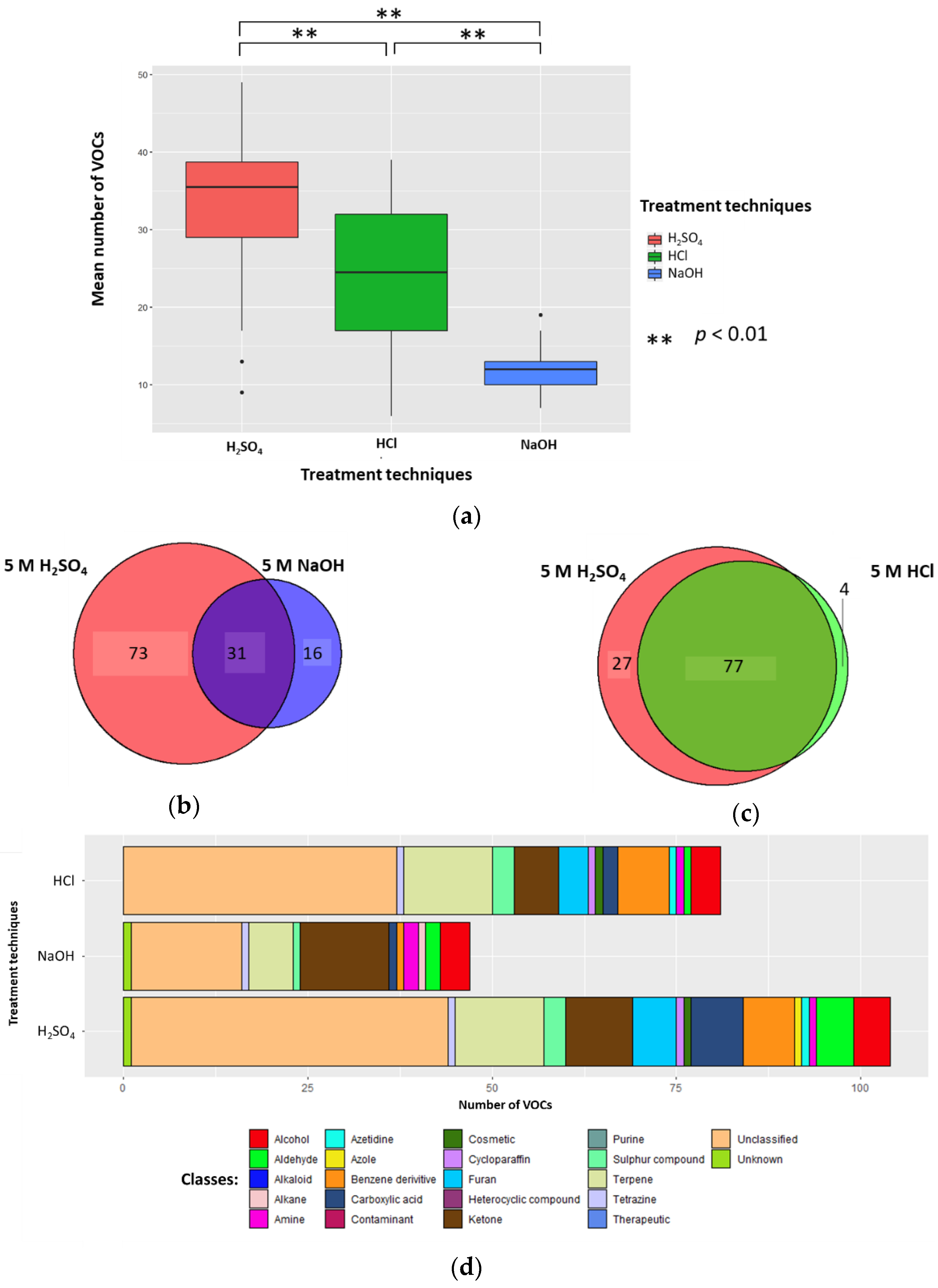
2.1. Altering Urine Sample pH by the Addition of 5 M H2SO4, 5 M HCl, or 5 M NaOH
2.1.1. Number of VOCs
2.1.2. Classification of VOCs
2.1.3. HS-SPME-GC-MS Degradation
2.1.4. Conclusion on Altering Sample pH
2.2. Altering Concentration of H2SO4
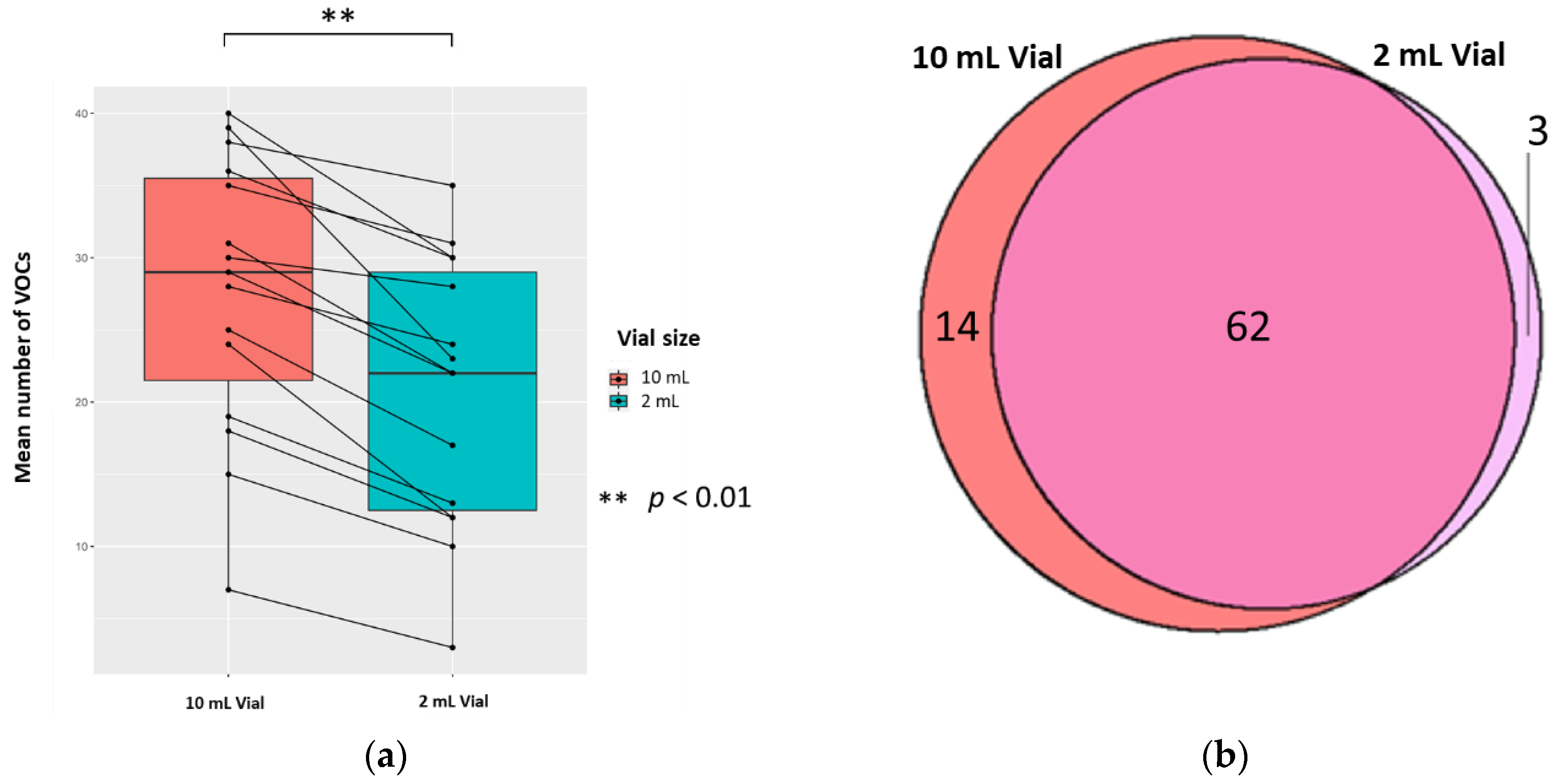
2.3. Altering Phase Ratio of H2SO4 Treated Urine Samples via Altering Vial Volume and Volume of Urine
2.3.1. The Vial Size
2.3.2. The Volume of Urine
3. Discussion
4. Materials and Methods
4.1. Donor Recruitment and Ethical Consent
4.2. Urine Samples
4.3. Chemicals and Materials
4.4. Experimental Conditions
4.4.1. Altering Sample pH (and Ionic Strength)
4.4.2. Altering Concentration of H2SO4
4.4.3. Altering Phase Ratio by Changing Vial Size
4.4.4. Altering Phase Ratio by Changing the Sample Volume
4.5. Static Headspace-SPME-GC-MS Analysis
4.6. Library Building
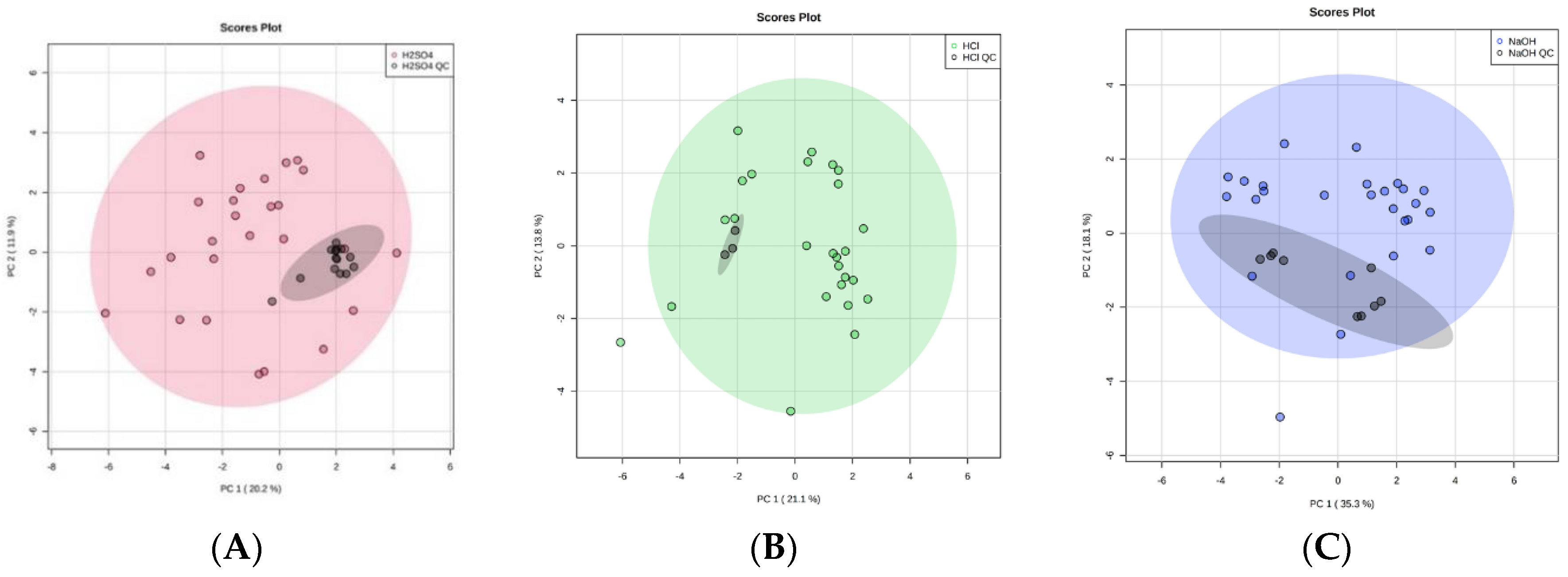
4.7. System Suitability and Quality Control
4.8. Equipment Stability of the HS-SPME-GC-MS over Time
4.9. Compound Identification
4.10. HS-SPME-GC-MS Degradation
5. Conclusions
Supplementary Materials
Author Contributions
Funding
Acknowledgments
Conflicts of Interest
References
- Gao, Q.; Lee, W.-Y. Urinary metabolites for urological cancer detection: A review on the application of volatile organic compounds for cancers. Am. J. Clin. Exp. Urol. 2019, 7, 232–248. [Google Scholar]
- Raftery, D. Mass Spectrometry in Metabolomics: Methods and Protocols; Humana Press: Totowa, NJ, USA, 2014. [Google Scholar] [CrossRef]
- Patti, G.J.; Yanes, O.; Siuzdak, G. Metabolomics: The apogee of the omics trilogy. Nat. Rev. Mol. Cell Biol. 2012, 13, 263–269. [Google Scholar] [CrossRef] [PubMed]
- Zhang, S.; Raftery, D. Headspace SPME-GC-MS Metabolomics Analysis of Urinary Volatile Organic Compounds (VOCs); Springer: New York, NY, USA, 2014; pp. 265–272. [Google Scholar] [CrossRef]
- Hough, R.; Archer, D.; Probert, C. A comparison of sample preparation methods for extracting volatile organic compounds (VOCs) from equine faeces using HS-SPME. Metabolomics 2018, 14, 19. [Google Scholar] [CrossRef] [PubMed]
- Aggio, R.B.; Mayor, A.; Coyle, S.; Reade, S.; Khalid, T.; Ratcliffe, N.M.; Probert, C.S. Freeze-drying: An alternative method for the analysis of volatile organic compounds in the headspace of urine samples using solid phase micro-extraction coupled to gas chromatography-mass spectrometry. Chem Cent. J. 2016, 10, 9. [Google Scholar] [CrossRef] [PubMed]
- Mills, G.A.; Walker, V. Headspace solid-phase microextraction profiling of volatile compounds in urine: Application to metabolic investigations. J. Chromatogr. B Biomed. Sci. Appl. 2001, 753, 259–268. [Google Scholar] [CrossRef]
- Smith, S.; Burden, H.; Persad, R.; Whittington, K.; De Lacy Costello, B.; Ratcliffe, N.M.; Probert, C.S. A comparative study of the analysis of human urine headspace using gas chromatography–mass spectrometry. J. Breath Res. 2008, 2, 037022. [Google Scholar] [CrossRef]
- Ahmed, I.; Greenwood, R.; Costello, B.d.L.; Ratcliffe, N.M.; Probert, C.S. An Investigation of Fecal Volatile Organic Metabolites in Irritable Bowel Syndrome. PLoS ONE 2013, 8, e58204. [Google Scholar] [CrossRef]
- Ahmed, I.; Greenwood, R.; Costello, B.; Ratcliffe, N.; Probert, C.S. Investigation of faecal volatile organic metabolites as novel diagnostic biomarkers in inflammatory bowel disease. Aliment. Pharmacol. Ther. 2016, 43, 596–611. [Google Scholar] [CrossRef]
- Zhuang, X.; Li, T.; Li, M.; Huang, S.; Qiu, Y.; Feng, R.; Zhang, S.; Chen, M.; Xiong, L.; Zeng, Z. Systematic Review and Meta-analysis: Short-Chain Fatty Acid Characterization in Patients With Inflammatory Bowel Disease. Inflamm. Bowel Dis. 2019, 25, 1751–1763. [Google Scholar] [CrossRef]
- Bond, A.; Greenwood, R.; Lewis, S.; Corfe, B.; Sarkar, S.; O’Toole, P.; Rooney, P.; Burkitt, M.; Hold, G.; Probert, C. Volatile organic compounds emitted from faeces as a biomarker for colorectal cancer. Aliment. Pharmacol. Ther. 2019, 49, 1005–1012. [Google Scholar] [CrossRef]
- Dospinescu, V.M.; Tiele, A.; Covington, J.A. Sniffing Out Urinary Tract Infection-Diagnosis Based on Volatile Organic Compounds and Smell Profile. Biosensors 2020, 10, 83. [Google Scholar] [CrossRef] [PubMed]
- Liu, D.; Zhao, N.; Wang, M.; Pi, X.; Feng, Y.; Wang, Y.; Tong, H.; Zhu, L.; Wang, C.; Li, E. Urine volatile organic compounds as biomarkers for minimal change type nephrotic syndrome. Biochem. Biophys. Res. Commun. 2018, 496, 58–63. [Google Scholar] [CrossRef] [PubMed]
- Kind, T.; Tolstikov, V.; Fiehn, O.; Weiss, R.H. A comprehensive urinary metabolomic approach for identifying kidney cancerr. Anal. Biochem. 2007, 363, 185–195. [Google Scholar] [CrossRef] [PubMed]
- Monteiro, M.; Moreira, N.; Pinto, J.; Pires-Luís, A.S.; Henrique, R.; Jerónimo, C.; Bastos, M.L.; Gil, A.M.; Carvalho, M.; Guedes de Pinho, P. GC-MS metabolomics-based approach for the identification of a potential VOC-biomarker panel in the urine of renal cell carcinoma patients. J. Cell. Mol. Med. 2017, 21, 2092–2105. [Google Scholar] [CrossRef] [PubMed]
- Zhou, Y.; Song, R.; Ma, C.; Zhou, L.; Liu, X.; Yin, P.; Zhang, Z.; Sun, Y.; Xu, C.; Lu, X.; et al. Discovery and validation of potential urinary biomarkers for bladder cancer diagnosis using a pseudotargeted GC-MS metabolomics method. Oncotarget 2017, 8, 20719–20728. [Google Scholar] [CrossRef] [PubMed]
- Janfaza, S.; Khorsand, B.; Nikkhah, M.; Zahiri, J. Digging deeper into volatile organic compounds associated with cancer. Biol. Methods Protoc. 2019, 4. [Google Scholar] [CrossRef]
- Lubes, G.; Goodarzi, M. GC–MS based metabolomics used for the identification of cancer volatile organic compounds as biomarkers. J. Pharm. Biomed. Anal. 2018, 147, 313–322. [Google Scholar] [CrossRef]
- Yusof, H.M.; Ab-Rahim, S.; Suddin, L.S.; Saman, M.S.A.; Mazlan, M. Metabolomics Profiling on Different Stages of Colorectal Cancer: A Systematic Review. Malays. J. Med. Sci. 2018, 25, 16–34. [Google Scholar] [CrossRef]
- Opitz, P.; Herbarth, O. The volatilome—Investigation of volatile organic metabolites (VOM) as potential tumor markers in patients with head and neck squamous cell carcinoma (HNSCC). J. Otolaryngol. Head Neck Surg. 2018, 47. [Google Scholar] [CrossRef]
- Janssens, E.; van Meerbeeck, J.P.; Lamote, K. Volatile organic compounds in human matrices as lung cancer biomarkers: A systematic review. Crit. Rev. Oncol. Hematol. 2020, 153, 103037. [Google Scholar] [CrossRef]
- De Lacy Costello, B.; Amann, A.; Al-Kateb, H.; Flynn, C.; Filipiak, W.; Khalid, T.; Osborne, D.; Ratcliffe, N.M. A review of the volatiles from the healthy human body. J. Breath Res. 2014, 8, 014001. [Google Scholar] [CrossRef] [PubMed]
- Demeestere, K.; Dewulf, J.; De Witte, B.; Van Langenhove, H. Sample preparation for the analysis of volatile organic compounds in air and water matrices. J. Chromatogr. A 2007, 1153, 130–144. [Google Scholar] [CrossRef] [PubMed]
- Asimakopoulos, A.D.; Del Fabbro, D.; Miano, R.; Santonico, M.; Capuano, R.; Pennazza, G.; D’Amico, A.; Finazzi-Agrò, E. Prostate cancer diagnosis through electronic nose in the urine headspace setting: A pilot study. Prostate Cancer Prostatic Dis. 2014, 17, 206–211. [Google Scholar] [CrossRef] [PubMed]
- Chandran, D.; Ooi, E.H.; Watson, D.I.; Kholmurodova, F.; Jaenisch, S.; Yazbeck, R. The Use of Selected Ion Flow Tube-Mass Spectrometry Technology to Identify Breath Volatile Organic Compounds for the Detection of Head and Neck Squamous Cell Carcinoma: A Pilot Study. Medicina 2019, 55, 306. [Google Scholar] [CrossRef] [PubMed]
- Pitt, J.J. Principles and applications of liquid chromatography-mass spectrometry in clinical biochemistry. Clin. Biochem. Rev. 2009, 30, 19–34. [Google Scholar] [PubMed]
- Câmara, J.S.; Alves, M.A.; Marques, J.C. Development of headspace solid-phase microextraction-gas chromatography–mass spectrometry methodology for analysis of terpenoids in Madeira wines. Anal. Chim. Acta 2006, 555, 191–200. [Google Scholar] [CrossRef]
- Emwas, A.-H.M. The Strengths and Weaknesses of NMR Spectroscopy and Mass Spectrometry with Particular Focus on Metabolomics Research; Springer: New York, NY, USA, 2015; pp. 161–193. [Google Scholar] [CrossRef]
- Arthur, C.L.; Pawliszyn, J. Solid phase microextraction with thermal desorption using fused silica optical fibers. Anal. Chem. 1990, 62, 2145–2148. [Google Scholar] [CrossRef]
- Cozzolino, R.; Giulio, B.; Marena, P.; Martignetti, A.; Günther, K.; Lauria, F.; Russo, P.; Stocchero, M.; Siani, A. Urinary volatile organic compounds in overweight compared to normal-weight children: Results from the Italian I.Family cohort. Sci. Rep. 2017, 7. [Google Scholar] [CrossRef]
- Bouatra, S.; Aziat, F.; Mandal, R.; Guo, A.C.; Wilson, M.R.; Knox, C.; Bjorndahl, T.C.; Krishnamurthy, R.; Saleem, F.; Liu, P.; et al. The human urine metabolome. PLoS ONE 2013, 8, e73076. [Google Scholar] [CrossRef]
- Mochalski, P.; King, J.; Klieber, M.; Unterkofler, K.; Hinterhuber, H.; Baumann, M.; Amann, A. Blood and breath levels of selected volatile organic compounds in healthy volunteers. Analyst 2013, 138, 2134–2145. [Google Scholar] [CrossRef]
- Turi, K.N.; Romick-Rosendale, L.; Ryckman, K.K.; Hartert, T.V. A review of metabolomics approaches and their application in identifying causal pathways of childhood asthma. J. Allergy Clin. Immun. 2018, 141, 1191–1201. [Google Scholar] [CrossRef] [PubMed]
- Buljubasic, F.; Buchbauer, G. The scent of human diseases: A review on specific volatile organic compounds as diagnostic biomarkers. Flavour Fragr. J. 2015, 30, 5–25. [Google Scholar] [CrossRef]
- Cozzolino, R.; De Magistris, L.; Saggese, P.; Stocchero, M.; Martignetti, A.; Di Stasio, M.; Malorni, A.; Marotta, R.; Boscaino, F.; Malorni, L. Use of solid-phase microextraction coupled to gas chromatography–mass spectrometry for determination of urinary volatile organic compounds in autistic children compared with healthy controls. Anal. Bioanal. Chem. 2014, 406, 4649–4662. [Google Scholar] [CrossRef] [PubMed]
- Schmidt, K.; Podmore, I. Current Challenges in Volatile Organic Compounds Analysis as Potential Biomarkers of Cancer. J. Biomark. 2015, 2015, 1–16. [Google Scholar] [CrossRef]
- Drabińska, N.; Starowicz, M.; Krupa-Kozak, U. Headspace Solid-Phase Microextraction Coupled with Gas Chromatography–Mass Spectrometry for the Determination of Volatile Organic Compounds in Urine. J. Anal. Chem. 2020, 75, 792–801. [Google Scholar] [CrossRef]
- Silva, C.L.; Passos, M.; Camara, J.S. Solid phase microextraction, mass spectrometry and metabolomic approaches for detection of potential urinary cancer biomarkers—a powerful strategy for breast cancer diagnosis. Talanta 2012, 89, 360–368. [Google Scholar] [CrossRef]
- Cho, D.-H.; Kong, S.-H.; Oh, S.-G. Analysis of trihalomethanes in drinking water using headspace-SPME technique with gas chromatography. Water Res. 2003, 37, 402–408. [Google Scholar] [CrossRef]
- Amaro, F.; Pinto, J.; Rocha, S.; Araújo, A.M.; Miranda-Gonçalves, V.; Jerónimo, C.; Henrique, R.; de Lourdes Bastos, M.; Carvalho, M.; de Pinho, P.G. Volatilomics Reveals Potential Biomarkers for Identification of Renal Cell Carcinoma: An In Vitro Approach. Metabolites 2020, 10, 174. [Google Scholar] [CrossRef]
- Hua, Q.; Wang, L.; Liu, C.; Han, L.; Zhang, Y.; Liu, H. Volatile metabonomic profiling in urine to detect novel biomarkers for B-cell non-Hodgkin’s lymphoma. Oncol. Lett. 2018, 15, 7806–7816. [Google Scholar] [CrossRef]
- Khalid, T.; Aggio, R.; White, P.; De Lacy Costello, B.; Persad, R.; Al-Kateb, H.; Jones, P.; Probert, C.S.; Ratcliffe, N. Urinary Volatile Organic Compounds for the Detection of Prostate Cancer. PLoS ONE 2015, 10, e0143283. [Google Scholar] [CrossRef]
- Mazzone, P.J.; Wang, X.F.; Lim, S.; Choi, H.; Jett, J.; Vachani, A.; Zhang, Q.; Beukemann, M.; Seeley, M.; Martino, R.; et al. Accuracy of volatile urine biomarkers for the detection and characterization of lung cancer. BMC Cancer 2015, 15, 1001. [Google Scholar] [CrossRef] [PubMed]
- Rodrigues, D.; Pinto, J.; Araújo, A.M.; Monteiro-Reis, S.; Jerónimo, C.; Henrique, R.; de Lourdes Bastos, M.; de Pinho, P.G.; Carvalho, M. Volatile metabolomic signature of bladder cancer cell lines based on gas chromatography–mass spectrometry. Metabolomics 2018, 14, 62. [Google Scholar] [CrossRef] [PubMed]
- Silva, C.L.; Passos, M.; Câmara, J.S. Investigation of urinary volatile organic metabolites as potential cancer biomarkers by solid-phase microextraction in combination with gas chromatography-mass spectrometry. Br. J. Cancer 2011, 105, 1894–1904. [Google Scholar] [CrossRef] [PubMed]
- Bonadio, F.; Margot, P.; Delémont, O.; Esseiva, P. Headspace solid-phase microextraction (HS-SPME) and liquid-liquid extraction (LLE): Comparison of the performance in classification of ecstasy tablets. Part 2. Forensic. Sci. Int. 2008, 182, 52–56. [Google Scholar] [CrossRef] [PubMed]
- Doong, R.-A.; Chang, S.-M.; Sun, Y.-C. Solid-Phase Microextraction and Headspace Solid-Phase Microextraction for the Determination of High Molecular-Weight Polycyclic Aromatic Hydrocarbons in Water and Soil Samples. J. Chromatogr. Sci. 2000, 38, 528–534. [Google Scholar] [CrossRef][Green Version]
- Drabińska, N.; Młynarz, P.; de Lacy Costello, B.; Jones, P.; Mielko, K.; Mielnik, J.; Persad, R.; Ratcliffe, N.M. An Optimization of Liquid–Liquid Extraction of Urinary Volatile and Semi-Volatile Compounds and Its Application for Gas Chromatography-Mass Spectrometry and Proton Nuclear Magnetic Resonance Spectroscopy. Molecules 2020, 25, 3651. [Google Scholar] [CrossRef]
- Tipler, A. An Introduction to Headspace Sampling in Gas Chromatography Fundamentals and Theory; Perkinelmer: Waltham, MA, USA, 2013. [Google Scholar]
- Dunn, W.B.; Wilson, I.D.; Nicholls, A.W.; Broadhurst, D. The importance of experimental design and QC samples in large-scale and MS-driven untargeted metabolomic studies of humans. Bioanalysis 2012, 4, 2249–2264. [Google Scholar] [CrossRef]
- Broadhurst, D.; Goodacre, R.; Reinke, S.N.; Kuligowski, J.; Wilson, I.D.; Lewis, M.R.; Dunn, W.B. Guidelines and considerations for the use of system suitability and quality control samples in mass spectrometry assays applied in untargeted clinical metabolomic studies. Metabolomics 2018, 14, 72. [Google Scholar] [CrossRef]
- Dudzik, D.; Barbas-Bernardos, C.; Garcia, A.; Barbas, C. Quality assurance procedures for mass spectrometry untargeted metabolomics. A review. J. Pharm. Biomed. Anal. 2018, 147, 149–173. [Google Scholar] [CrossRef]
- Khodadadi, M.; Pourfarzam, M. A review of strategies for untargeted urinary metabolomic analysis using gas chromatography-mass spectrometry. Metabolomics 2020, 16, 66. [Google Scholar] [CrossRef]
- Aggio, R.; Villas-Boas, S.G.; Ruggiero, K. Metab: An R package for high-throughput analysis of metabolomics data generated by GC-MS. Bioinformatics 2011, 27, 2316–2318. [Google Scholar] [CrossRef] [PubMed]
- Chong, J.; Soufan, O.; Li, C.; Caraus, I.; Li, S.; Bourque, G.; Wishart, D.S.; Xia, J. MetaboAnalyst 4.0: Towards more transparent and integrative metabolomics analysis. Nucleic Acids Res. 2018, 46, W486–W494. [Google Scholar] [CrossRef] [PubMed]
- R Core Team. A Language and Environment for Statistical Computing; R Foundation for Statistical Computing: Vienna, Austria, 2014. [Google Scholar]
- Chen, H.; Boutros, P.C. VennDiagram: A package for the generation of highly-customizable Venn and Euler diagrams in R. BMC Bioinform. 2011, 12, 35. [Google Scholar] [CrossRef] [PubMed]
- National Library of Medicine. Medical Subject Headings. Available online: https://www.nlm.nih.gov/mesh/meshhome.html (accessed on 23 September 2020).


| Retention Time (min) | Compound Name (IUPAC Name) | H2SO4 v HCl 1 | H2SO4 v NaOH 1 |
|---|---|---|---|
| 16.53 | dihydroxy(dimethyl)silane | - | <0.01 |
| 16.93 | 2,2,4,4,6,6-hexamethyl-1,3,5,2,4,6-trioxatrisilinane | <0.01 | >0.01 |
| 23.1 | 2,2,4,4,6,6,8,8-octamethyl-1,3,5,7,2,4,6,8-tetraoxatetrasilocane | <0.01 | >0.01 |
| 24.03 | [(dimethyl-3-silanyl)oxy-dimethylsilyl]oxy-dimethylsilicon | <0.01 | - |
| 24.3 | trimethoxy(methyl)silane | - | - |
| 28.51 | 2-Hydroxymandelic acid, ethyl ester, di-TMS | >0.01 | >0.01 |
| 28.51_2 | 2,4-bis(trimethylsilyloxy)benzaldehyde | <0.01 | <0.01 |
| 28.53 | Tetramethylsilane | <0.01 | <0.01 |
| 29.28 | 2,2,4,4,6,6-hexamethyl-1,3,5,2,4,6-trioxatrisilinane | - | <0.01 |
| 33.87 | Tetramethylsilane | >0.01 | >0.01 |
| 36.56 | trimethyl(1-trimethylsilylethyl)silane | >0.01 | - |
| 38.75 | bis[[dimethyl(trimethylsilyloxy)silyl]oxy]-dimethylsilane | <0.01 | <0.01 |
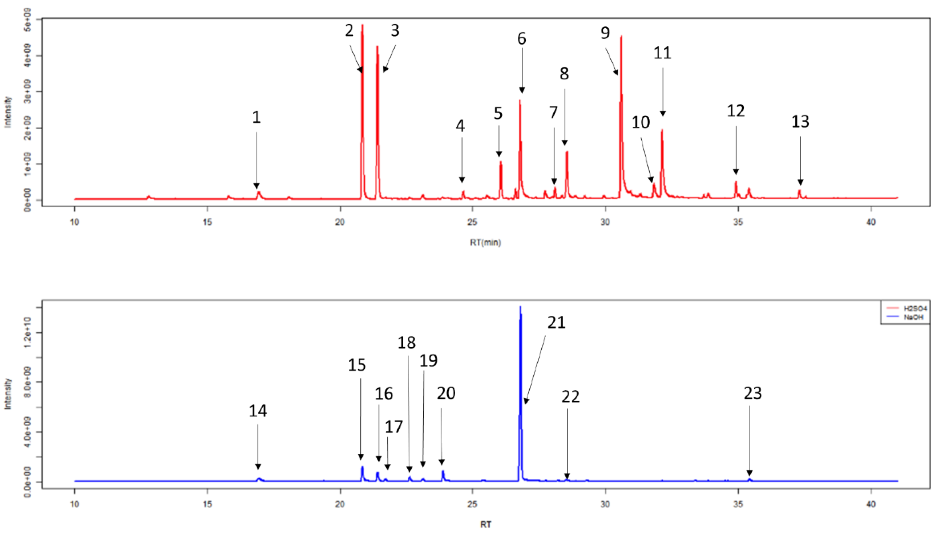
| Label | Retention Time (min) | Compound Name (IUPAC Name) |
|---|---|---|
| 1 | 16.93 | 2,2,4,4,6,6-hexamethyl-1,3,5,2,4,6-trioxatrisilinane (Contaminant) * |
| 2 | 20.88 | heptan-4-one * |
| 3 | 21.44 | heptan-3-one * |
| 4 | 24.67 | 2-methyl-5-methylsulfanylfuran |
| 5 | 26.01 | 1-methyl-4-propan-2-ylbenzene (p-Cimene) |
| 6 | 26.93 | 2-ethylhexan-1-ol * |
| 7 | 27.76 | Phenol |
| 8 | 28.55 | 1-methyl-4-prop-1-en-2-ylbenzene-or-1-methyl-2-prop-1-en-2-ylbenzene |
| 9 | 30.61 | 4-methylphenol |
| 10 | 31.83 | (1R,2R,5R)-5-methyl-2-propan-2-ylcyclohexan-1-ol |
| 11 | 32.14 | 5-methyl-2-propan-2-ylcyclohexan-1-ol(Menthol) |
| 12 | 35.42 | 3-methyl-6-propan-2-ylcyclohex-2-en-1-one * |
| 13 | 37.32 | 2-buta-1,3-dienyl-1,3,5-trimethylbenzene |
| 14 | 16.93 | 2,2,4,4,6,6-hexamethyl-1,3,5,2,4,6-trioxatrisilinane (Contaminant) * |
| 15 | 20.88 | heptan-4-one * |
| 16 | 21.44 | heptan-3-one * |
| 17 | 21.71 | heptan-2-one |
| 18 | 22.61 | (E)-2-methylhept-2-enal |
| 19 | 23.10 | 2,2,4,4,6,6,8,8-octamethyl-1,3,5,7,2,4,6,8-tetraoxatetrasilocane (Contaminant) * |
| 20 | 23.91 | Oxime-, methoxy-phenyl-(Contaminant) |
| 21 | 26.93 | 2-ethylhexan-1-ol * |
| 22 | 28.53 | Tetramethylsilane (TMS) (Contaminant) |
| 23 | 35.42 | 3-methyl-6-propan-2-ylcyclohex-2-en-1-one * |
Publisher’s Note: MDPI stays neutral with regard to jurisdictional claims in published maps and institutional affiliations. |
© 2020 by the authors. Licensee MDPI, Basel, Switzerland. This article is an open access article distributed under the terms and conditions of the Creative Commons Attribution (CC BY) license (http://creativecommons.org/licenses/by/4.0/).
Share and Cite
Aggarwal, P.; Baker, J.; Boyd, M.T.; Coyle, S.; Probert, C.; Chapman, E.A. Optimisation of Urine Sample Preparation for Headspace-Solid Phase Microextraction Gas Chromatography-Mass Spectrometry: Altering Sample pH, Sulphuric Acid Concentration and Phase Ratio. Metabolites 2020, 10, 482. https://doi.org/10.3390/metabo10120482
Aggarwal P, Baker J, Boyd MT, Coyle S, Probert C, Chapman EA. Optimisation of Urine Sample Preparation for Headspace-Solid Phase Microextraction Gas Chromatography-Mass Spectrometry: Altering Sample pH, Sulphuric Acid Concentration and Phase Ratio. Metabolites. 2020; 10(12):482. https://doi.org/10.3390/metabo10120482
Chicago/Turabian StyleAggarwal, Prashant, James Baker, Mark T. Boyd, Séamus Coyle, Chris Probert, and Elinor A. Chapman. 2020. "Optimisation of Urine Sample Preparation for Headspace-Solid Phase Microextraction Gas Chromatography-Mass Spectrometry: Altering Sample pH, Sulphuric Acid Concentration and Phase Ratio" Metabolites 10, no. 12: 482. https://doi.org/10.3390/metabo10120482
APA StyleAggarwal, P., Baker, J., Boyd, M. T., Coyle, S., Probert, C., & Chapman, E. A. (2020). Optimisation of Urine Sample Preparation for Headspace-Solid Phase Microextraction Gas Chromatography-Mass Spectrometry: Altering Sample pH, Sulphuric Acid Concentration and Phase Ratio. Metabolites, 10(12), 482. https://doi.org/10.3390/metabo10120482