Dissecting Tether’s Nonlinear Dynamics during Covid-19

Abstract

The present study is on the five cryptocurrency daily mean return time series linearity dynamics during the Covid-19 period. These cryptocurrencies were chosen based on their influence on the market, primarily driven by its market capitalisation. Tether is included as the most important stable coin on the market, nominally pegged to the U.S. dollar (USD). The reason to investigate it is that there are some inconsistencies in its behaviour as opposed to the other four cryptocurrencies. This study found that the behaviour of Tether cryptocurrency daily average return time series pattern is highly nonlinear and chaotic in nature, whereas the other four cryptocurrencies (namely Bitcoin, Ethereum, XRP and Bitcoin Cash) daily average return time series were found to be linear in nature. To further study Tether’s nonlinear time series rich dynamics, this study deployed one category of the regime switching models popularly known as the threshold regressions. The study estimates fairly suggest that both the threshold autoregression (TAR) and smooth transition autoregressive (STAR) models with lag 1 are adequate to capture the rich nonlinear and chaotic dynamics of Tether’s daily average return time series.

1. Introduction

Over the last few decades, there has been a significant increase in the number of studies that focus primarily on the cause and effect of crises on the financial markets across the globe. Those studies highlighted that a financial crisis has significantly negative effects on the global financial markets [1,2,3,4,5,6]. On the other hand, it also highlighted that risk and risk premiums associated with the different industry sectors vary explicitly during crises. All these studies unanimously emphasized the existence of asymmetric and nonlinear dynamics of the financial markets. Since the Great Depression of the 1930s, studies in economics and econometrics have tried to figure out whether “economic variables exhibit nonlinear behaviour during crisis”. During the recent global crisis of 2008–2009, all financial markets were strongly affected despite strong intervention and support from the government and central banks. Financial shocks during the global crisis of 2008–2009 induced strong negative impacts to the macroeconomic variables. This indicates a strong linkage between the financial market and macroeconomic variables. A seminal study [7] confirmed that business cycle asymmetries are reflected in several economic variables such as: employment, industrial productions etc. After that, some studies [8,9,10] discovered different variants of asymmetries or nonlinearity other than business cycle, such as bi-linearity, regime switching, structural breaks, and conditional volatility in stock returns, interest rates, and exchange rates respectively. Such nonlinear behaviour of the time series variable indicates interesting, stylised facts about the variable with an importance to identify such stylised facts for three reasons: data accuracy and validation; model misspecifications; and accurate policy modelling. The theoretical foundation for the same behaviour today is also well regarded in finance. Markowitz portfolio selection theory based on mean-variance frontier assumes a perfect capital market with risk averse investors, and states that adding randomly selected and equally weighted assets to a portfolio leads to a risk reduction. However, [11,12] highlighted interestingly that the presence of marginal asymmetry in the time series returns could fundamentally affect overall portfolio diversifications. All these above points indicate that the stylized facts on the time series asymmetry/nonlinearity is very useful. To obtain such stylized facts on nonlinearity of the time series, appropriate statistical methods should be implemented. Unfortunately, this is not always the case in practice as detailed by Vavra [13].

S. Ulam, a Noble laureate, expressed “Using the term non-linear to describe a time series is like saying that zoology is the study of non-elephant animals.” This quote illustrates the common problem associated with nonlinear theory, testing, methods, and modelling. The field of nonlinearity is so vast that it is very difficult to generalise the theory, functions, or models as similar to the existing linear functions or models. Fortunately, the last few decades have witnessed continuous developments in the theories and functions/models related to the “non-elephant”. Analysing economic and financial asymmetry/nonlinearity time series in particular is very difficult mainly due to three reasons: dependency, outliers, and fat tails. Most of the studies today are limited to analyse nonlinear characteristics of the economic variables and financial markets assets. One such important asset class in the financial market are cryptocurrencies that have very distinctive features. The development of cryptocurrency leads to financial and monetary innovation. Cryptocurrency has several features like a currency, as well as several features of available financial assets. Hence cryptocurrency cannot be categorised exclusively either as currency or other available financial asset classes. Distinctive or peculiar features of the cryptocurrencies cannot be fully captured by the traditional theories or methods, but rather demand more sophisticated analysis. Although the last few years have witnessed a significant increase in the number of studies related to cryptocurrency, studies related to nonlinear behaviour of cryptocurrency time series is almost untouched. With this backdrop, the present study is engaged to fill all such gaps in the prevailing literature on asymmetry/nonlinearity. Firstly, the study analyses the behaviour of the five major cryptocurrencies, namely Bitcoin, Ethereum, XRP, Tether, and Bitcoin cash, during the Covid-19 crisis. Second, the study checks whether the behaviour or nature of all five cryptocurrencies were similar during the Covid-19 crisis regarding linear and nonlinear characteristics. Third, if any cases of asymmetric/nonlinear nature or behaviour arose among the five major cryptocurrencies, then the study will further investigate critically such behaviour or nature. Fourth, the study analyses such asymmetric/nonlinear nature or behaviour by deploying suitable techniques to test nonlinearity such as threshold regression.

The goal of this study is to test linear and nonlinear behaviour of daily average returns of Bitcoin, Ethereum, XRP, Tether, and Bitcoin cash during the Covid-19 crisis. In the case of nonlinearity, the next goal of the study is testing daily returns time series in the regime switching models. The contribution of this study is in the fact that these models were used previously in several studies. Because of that, there is still a gap in scientific literacy about this topic about whether nonlinear models are efficient in testing regression of daily cryptocurrency returns. The results of this work can be insights for the future studies to investigate what models outperform (linear or nonlinear) for different cryptocurrencies.

2. Literature Review

Most researches in financial time series use linear models like Box–Jenkins [14], different autoregressive conditional heteroskedasticity (ARCH) models [15], the Markov model [16], and many other variations of such models to study and forecast stationary processes and the variance of error values. These models are limited to explain nonlinear behavior of values [17]. In 1990, Tong introduced the threshold autoregressive (TAR) model [18,19], which provides an extensive set of possible dynamics for financial and economic time series compared with different ARCH models. The first authors who confirmed this feature of TAR were Li and Lam [20], by measuring asymmetry of stock returns on high volatile markets. After, similar studies were conducted by [21,22]. Some authors used regression trees models [18], which are closely related to the TAR model, and threshold autoregression modifications like the smooth transition threshold model (STAR) by Chan and Tong [23]. Hansen [24] used TAR to study the different stages in economic growth models, while Chen et al. [25] used TAR to analyze stock returns and volatilities. The TAR model has very important features: (a) it is essentially simple as a linear model [26], (b) but it also captures nonlinear phenomena like asymmetries [26], business cycles [24], monetary researches [27,28], and other nonlinear phenomena that can be significant especially in crises.

However, TAR models are not used in mass finance research because it is difficult to find an appropriate threshold variable, or such variables cause high measurement errors [26]. Such errors could lead to loss of information or deceptive conclusions [26,29] and influence on TAR models being too restrictive in existent applications. Less restrictive TAR variation models are STAR models: the logistic STAR model (LSTAR) and the exponential STAR model (ESTAR). The difference between these two models is that LSTAR is a special case of the single threshold TAR model and ESTAR is a variant of a double-threshold TAR model. According to Teräsvirta [30], if linearity is rejected, then only the STAR model is appropriate. The same author argued that the STAR model is very useful in the case when many economic agents make decisions and influence results in time series. Their dichotomous decisions are less likely influenced by discrete behavior; they are rather smooth than discrete. The STAR model is useful to explain nonlinear dynamics of financial and economic time series. In the study of Teräsvirta et al. [31], the STAR model outperforms linear autoregressive (AR) models in forecasting 47 macroeconomic variables of G7 countries. There are only few studies where TAR and STAR models are tested on cryptocurrency markets. Chen and Hafner [32] tested speculative bubbles on the cryptocurrency market using a smooth transition autoregressive. These authors argued that application of STAR model is very appropriate in the case when the price dynamics will be driven by an explosive autoregression. They used the sentiment index on the cryptocurrency market as a transition variable. Yang [33] used a STAR model with exogenous variables (STARX) to consider whether there is a nonlinear relationship between Bitcoin and Taiwan’s stock market. The same author (2020) tested a smooth transition autoregressive model and confirmed that it provides better predictive competence compared with a traditional linear model. Previously, this was proved in research by [27,28]. Yang [33] found a threshold effect and confirmed nonlinearity (2020). Mostly, authors used smooth transitions in other models, like smooth transition Generalized Autoregressive Conditionally Heteroskedastic (GARCH) models, to study asymmetric volatility in cryptocurrency markets [34]. Gong and Huser [35] applied asymmetric tail dependence models to test cryptocurrency market data. They also proposed a parsimonious copula model that keeps high flexibility in both the lower and upper tails of the cryptocurrency market. Similar research has previously been carried out by Huser and Wadsworth [36], whose model has shown high flexibility in the upper tails. Above all, studies evidence the crypto market is well known for its volatility, and it is primarily driven by its most famous currency, Bitcoin.

An important part of our study is a question of hedging capabilities within a crypto market, mainly because of their volatility driven by speculative motives and associated high level of risk. Tether is the only important stable coin on the crypto market with significant market capitalization, reaching at this moment almost 10 billion USD. Tether is purportedly backed by USD reserves, but there is no clear evidence for this, although crypto exchanges widely use Tether in transactions. Based on this behavior there is an idea to use Tether as a safe haven in the crypto market because of its specific characteristics as opposed to all other important cryptocurrencies, or at least to hedge the position with a certain proportion of Tether in the overall portfolio in cryptocurrencies. Looking at the current market data it is evident that in the last half of the year market capitalization of Tether has been increased more than doubled, from 4105 billion USD on 31 December 2019 to 9167 billion USD on 6 June 2020, with very high average volume in the overall period of approximately 50 billion USD per day. As the price of Tether is not volatile, it has been during the whole period in the range between 0.92 USD to 1.03 USD. It is obvious that there have been a lot of growing tokens issued and it is controversial that they are fully backed up with USD, as is claimed. Griffin and Shams [37] tested two hypotheses regarding the role of Tether in a crypto world, especially on Bitcoin. The first hypothesis was demand driven with the idea that Tether is being used as a medium of exchange to enter fiat currency in the crypto world. It was not supported, but there was noise. The second one was a hypothesis with an argument that Tether flows cause positive Bitcoin returns. The evident argument behind Tether is that it is being printed unbacked by USD and pushed out onto the market with an inflationary effect on asset prices. This is in accordance with a study done by Liu and Tsyvinski [38] which showed that none of the exposures to macroeconomic factors, stocks markets, currencies, or commodities can explain cryptocurrency prices. On the other hand, Griffin and Shams [37] in their study found that Tether has a sizable impact on Bitcoin prices. These findings are generally consistent with the evidence that sophisticated investors may profit from bubbles [39]. There has been a lot of controversy whether the organization behind Tether truly has enough USDs in reserve to cover the supply of Tether. According to Coin Telegraph, despite numerous statements by the Tether organization, there is serious doubt by members of the community that everything is legitimate [40]. Allen and Bryant [41] concluded that although the idea about introducing Tether is great in theory, and something like Tether may be the first step in widespread cryptocurrency adoption, it may need to come from an organization that is more trusted for innovation in space. Although extremely unlikely, if Tether were to become officially backed by the U.S. government, the issue some may have with trust could be resolved. Based on the current literature review, it seems that Tether is being used by a well-organized pull of investors to manipulate the crypto market, mainly Bitcoin, but there is now much evidence on it. The idea of the present study is to investigate this claim by testing the rich dynamics of nonlinear or the chaotic nature of time series of 5 cryptocurrencies, namely Bitcoin, Ethereum, XRP, Bitcoin cash, and Tether, and to see if there is some inconsistency with Tether as opposed to the other four major cryptocurrencies.

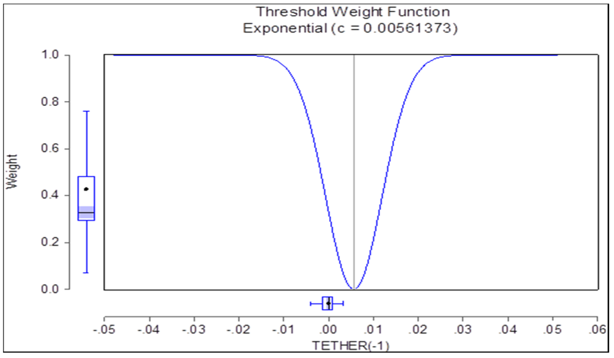
3. Data and Methodology

3.1. Data

The data regarding the top five cryptocurrencies, namely Bitcoin, Ethereum, XRP, Tether and Bitcoin cash, were obtained from CoinMarketCap website (https://coinmarketcap.com/). The data consisted of daily closing prices for a period from 31 December 2019 to 27 May 2020. From the daily closing pricing dataset daily, average returns were calculated for the period 1 January 2020 to 27 May 2020. This study defines this period (1 January 2020 to 27 May 2020) as the Covid-19 pandemic period with 148 total data points.

3.2. Methodology

This study used three stepwise methods to derive the results, as follows: test of stationarity (Augmented Dickey-Fuller (ADF) test); test of linearity (Brock, Dechert, Scheinkman and LeBaron (BDS) independence test); and nonlinear modelling using threshold regressions (threshold autoregression (TAR) model).

3.2.1. Test of Stationarity

This study used the Dickey-Fuller test (1979) to check the stationarity in the time series [42]. It compares the null hypothesis “time series has a unit root” to the alternative hypothesis “time series has no unit root”.

3.2.2. Test of Linearity

To check the linearity of the time series, this study used the Brock, Dechert, Scheinkman and LeBaron (1996) (BDS) test for independence, specifically the Epsilon method of “fraction of pairs” with a default value of Є = 0.7 [43]

3.2.3. Nonlinear Modelling Technique

To study the rich dynamics of nonlinear or chaotic nature of time series, this study deployed threshold regression. Following Hansen, Bruce (2011), the threshold autoregression (TAR) model is used to study the nonlinear relationship between the outcomes and different threshold regressors [44]. Threshold autoregression (TAR) models are one category of the regime switching models in which the slope of the parameters varies according to a switching regime mechanism based on the threshold variables. This allows us to study the asymmetric behaviours that exist in the time series that could not be enlightened by the Autoregressive Moving Average (ARMA) models. The threshold autoregression (TAR) model estimates an answer to two basic questions: (1) How to select the optimal threshold value and (2) how to select the optimal lag or delay value in nonlinear time series.

In general, a threshold regression is defined as follows:

$$\mathrm{yt}=\mathsf{\alpha }+\mathsf{\beta }{0}^{\prime }\mathrm{xt}+\mathsf{\beta }{1}^{\prime }\mathrm{xt}\mathrm{h}\left(\mathrm{qt}; \mathsf{\theta }\right)+\mathsf{\epsilon }\mathrm{t}$$

(1)

where yt is a dependable variable, α is regression intercept, β0 and β1 are K X 1 vectors, qt is a threshold variable, θ a vector of parameters, h (qt; θ) a transition function, and εt error terms.

Following Hansen and Bruce (2011), this study deployed a two-regime (lower and higher) threshold regression with AR (11) in each regime. For estimating threshold values, the study used techniques presented by Bai and Perron (1998) [45]. Model selection criteria was based on the sum squared residual value of the threshold regressions. Similar to the threshold autoregression (TAR) model, another very popular method is the smooth transition autoregressive (STAR) model that is also used as an application of the threshold regression to study the nonlinear time series rich dynamics. Smooth transition autoregressive (STAR) is a special case of smooth transition regression as suggested by Teräsvirta (1994). The STAR technique is very similar to TAR, except in case the STAR indicator function is replaced with the continuous transition function that returns values in between 0 and 1. The present study chose an exponential function as the transition function. The exponential transition function is represented as follows: G (s; c, γ) = 1− exp (−γ (s−c)2), where s is the threshold variable, c is the threshold value, and γ represents slope.

4. Results and Discussion

4.1. Preliminary Analysis

Analysis was initiated by looking into the descriptive statistics of the variables.

Table 1. Descriptive statistics.

	Bitcoin	Ethereum	XRP	Tether	Bitcoin Cash
Mean	0.002987	0.005318	0.001481	0.000036	0.003438
Std. Dev.	0.049043	0.061276	0.049437	0.008307	0.068998
Skewness	−2.495034	−1.874384	−1.683356	0.427823	−0.722019
Kurtosis	25.75436	19.180970	16.310970	19.438160	15.459380

shows descriptive statistics and Figure 1 shows cryptocurrency average daily returns. Table 1 estimates highlight that the values of kurtosis were very high for all cryptocurrencies time series of daily average returns [46,47]. Higher values of kurtosis indicate high level of investment risk in all of these five cryptocurrencies.

4.2. Unit Root Test

A unit root test, the Augmented Dickey-Fuller test (ADF Test), was run to check whether the time series were stationary or not. Estimates obtained from the Augmented Dickey-Fuller test (ADF Test) are shown in

Table 2. Augmented Dickey-Fuller test to check unit root presence.

	Bitcoin	Ethereum	Tether	XRP	Bitcoin Cash
t-Statistic	−14.238	−14.614	−8.344	−14.434	−14.509
Probability *	0.000	0.000	0.000	0.000	0.000

. The estimates show that the time series of all cryptocurrencies average returns reject the null hypothesis of “Time series has a unit root”. Hence it shows that all five cryptocurrencies return meet the condition of stationarity.

4.3. Linearity Test: BDS Independence Test

Thereafter a BDS independence test was run, as described by Brock, Dechert, Scheinkman and LeBaron (1996), to check whether the time series are linear or nonlinear.

Table 3. Brock, Dechert, Scheinkman and LeBaron (BDS) test of independence.

	Bitcoin	Ethereum	Tether	XRP	Bitcoin Cash
Dimension	Probability	Probability	Probability *	Probability	Probability
2	0.932	0.927	0.000	0.103	0.685
3	0.908	0.821	0.000	0.216	0.270
4	0.888	0.994	0.000	0.193	0.352
5	0.871	0.863	0.000	0.163	0.754
6	0.855	0.842	0.000	0.247	0.962

shows the estimates obtained from the BDS independence test for all five cryptocurrencies. In the case of Tether, as shown in Table 3, the BDS independence test estimates clearly rejected the null hypothesis of “time series is linearly dependent”, whereas the BDS independence test estimates failed to reject the null hypothesis of “time series are linearly dependent” for the other four cryptocurrencies. The BDS independence test estimates clearly indicate that the Tether daily average returns pattern was highly nonlinear and chaotic in nature.

4.4. Estimation of Nonlinear Models (Threshold Regressions)

4.4.1. Threshold Autoregression (TAR) Modelling

The above discussion indicate that the behaviour of the Tether daily average return time series is nonlinear and chaotic in nature. To analyse such a nonlinear and chaotic nature of Tether daily average return series study deployed a nonlinear technique, namely discrete threshold regression. Discrete threshold regression is very useful in describing “a simple form of nonlinear regression featuring piecewise linear specifications and regime switching that occurs when an observed variable crosses an unknown threshold”. The coefficients of the model might be constant in each regime but could change between the regimes. The main goal of the threshold regression is to estimate those value or values of the time series that trigger the regime change. The threshold autoregression (TAR) model is very popular among such as an application of threshold regression to study the nonlinear time series rich dynamics. Following Hansen and Bruce (2011), this study deployed a two-regime threshold regression with AR (11) in each regime and model selection criteria based over threshold dependent variables lags from −1 to −2. Two regimes of threshold autoregression (TAR) model estimates are represented in

Table 4. Threshold autoregression (TAR) model results.

Threshold Variable: Tether (−1)
Variable	Coefficient	Std. Error	t-Statistic	Prob.
Tether (−1) < −0.001140001—38 obs.
Tether (−1)	−0.10914	0.184903	−0.59023	0.5562
Tether (−2)	−0.07107	0.173475	−0.40971	0.6828
Tether (−3)	−0.26572	0.270092	−0.98381	0.3273
Tether (−4)	0.387365	0.246994	1.568321	0.1196
Tether (−5)	−0.06091	0.222329	−0.27395	0.7846
Tether (−6)	0.065645	0.269297	0.243765	0.8079
Tether (−7) *	0.677793	0.294807	2.299106	0.0233
Tether (−8) *	0.991814	0.296787	3.34184	0.0011
Tether (−9) *	1.034881	0.302744	3.418336	0.0009
Tether (−10)	−0.08355	0.160758	−0.51974	0.6043
Tether (−11) *	−0.57932	0.123476	−4.69175	0
−0.001140001 ≤ Tether (−1)—99 obs.
Tether (−1) *	−0.98163	0.087435	−11.227	0
Tether (−2)	−0.35435	0.181508	−1.95225	0.0534
Tether (−3) *	−0.36605	0.166612	−2.19703	0.03
Tether (−4) *	−0.40413	0.170195	−2.37451	0.0192
Tether (−5)	−0.24926	0.177464	−1.40459	0.1629
Tether (−6)	−0.1504	0.147985	−1.01629	0.3116
Tether (−7)	−0.1415	0.15486	−0.91371	0.3628
Tether (−8)	0.032204	0.155084	0.207654	0.8359
Tether (−9)	−0.01751	0.142241	−0.1231	0.9022
Tether (−10)	−0.04232	0.138461	−0.30565	0.7604
Tether (−11)	−0.01973	0.114225	−0.17274	0.8632
Non-Threshold Variables
C	0.001227	0.000559	2.194048	0.0303
R-squared	0.666588	Mean dependent var.		3.55E05
Adjusted R-squared	0.602245	S.D. dependent var.		0.008466
S.E. of regression	0.005339	Akaike info criterion		−7.4754
Sum squared residual	0.00325	Schwarz criterion		−6.98519
Log likelihood	535.065	Hannan-Quinn criteria		−7.27619
F-statistic	10.35997	Durbin-Watson stat		2.036223
Prob (F-statistic)	0

with lag 1. Threshold specification is estimated using techniques presented by Bai and Perron (1998) with trimming percentage of 15% and a significant level of 5%.

As shown above in Table 4, the two regimes are divided based on lower and upper threshold values. The model with lag 1 choses threshold value of −0.001140001; similarly, model 2 with lag 2 choses a threshold value of 0.0009529071. Then coefficient values for all threshold regressors Tether (−1 to −11) along with the associated statistics for each regime (1 and 2) are displayed. In this part summary statistics are self-explanatory and * represents respective threshold variable statistical significance at 5% level. The end of Table 4 shows the results for comparison with the fully restricted, no threshold, constant only model estimates. Durbin-Watson statistics confirm the absence of autocorrelation in the time series data. The R-squared value found to be 66.66% for the suggested model. Model selection criteria was based on lower value of the sum squared residual. Here, model 1 with lag 1 has a sum squared residual value of 0.00325, which is lower than the model 2 with lag 2 sum squared residual value of 0.003641. Hence a two-regime TAR model with lag 1 was chosen over lag 2.

4.4.2. Smooth Transition Autoregressive (STAR) Modelling

A two-regime (linear and nonlinear) threshold regression was then deployed, with six thresholds varying regressors in each regime with a lag of 1. STAR model estimates are shown below in

Table 5. Smooth transition autoregressive (STAR) model estimates.

Variable	Coefficient	Std. Error	t-Statistic	Prob.
Threshold Variables (linear part)
Tether (−1) *	−0.89612	0.236203	−3.79385	0.0002
Tether (−2)	−0.0959	0.298315	−0.32148	0.7484
Tether (−3)	−0.06499	0.284464	−0.22845	0.8197
Tether (−4)	−0.17043	0.281426	−0.60559	0.5459
Tether (−5)	0.018679	0.272179	0.068626	0.9454
Tether (−6)	0.161718	0.233173	0.693556	0.4892
Threshold Variables (nonlinear part)
Tether (−1)	0.091936	0.289676	0.317376	0.7515
Tether (−2)	−0.65714	0.367002	−1.79055	0.0757
Tether (−3)	−0.65235	0.419154	−1.55634	0.1221
Tether (−4)	0.038943	0.488094	0.079786	0.9365
Tether (−5)	−0.49741	0.437	−1.13823	0.2572
Tether (−6) *	−0.94691	0.353547	−2.67831	0.0084
Slopes	12671.02	9092.054	1.393637	0.1658
Thresholds
Thresholds	0.005614	0.00191	2.939473	0.0039
R-squared	0.48408	Mean dependent var		0.000035
Adjusted R-squared	0.431682	S.D. dependent var		0.008399
S.E. of regression	0.006332	Akaike info criterion		−7.19315
Sum squared residual	0.005131	Schwarz criterion		−6.90173
Log likelihood	524.7135	Hannan-Quinn criteria		−7.07473
Durbin-Watson stat	2.049758

.

Estimates show that estimation converges after 14 iterations. In this part, summary statistics are self-explanatory and * represents respective threshold variable statistical significance at 5% level. The end of Table 5 shows results for comparison with the fully restricted, no threshold, constant only model estimates.

Durbin-Watson statistics confirm the absence of autocorrelation in the time series data. The R-squared value was found to be 48.41% for the suggested model. Figure 2 shows the threshold weights view and shape of the smoothing function or the values of the smoothing weights for each observation in the estimation sample. From Figure 2, visually we can see that the median transition weight is near 0.0056 and nonlinear. Moreover, the weight function is V shaped with most of the variation occurring well within two standard deviations of the lagged daily change in the return.

Model selection criteria is based on the lower value of the sum squared residual, which is lower in case of lag 1.

Table 6. Linearity test estimates.

Linearity Tests
Null Hypothesis	F-Statistic	d.f.	p-Value
H04: b1 = b2 = b3 = b4 = 0	1.372383	(24, 112)	0.1373
H03: b1 = b2 = b3 = 0	1.750093	(18, 118)	0.0399
H02: b1 = b2 = 0	1.779543	(12, 124)	0.0585
H01: b1 = 0	2.964582	(6, 130)	0.0096

Note: Linear model is rejected at the 5% level using H03.

shows the estimates of the linearity tests against nonlinear alternatives using the selected threshold variable. The test estimates strongly reject the null of linearity against the smooth transition alternatives.

Table 7. Encapsulated nonlinearity test.

Encapsulated Nonlinearity Tests
Null Hypothesis	F-Statistic	d.f.	p-Value
H04: b1 = b2 = b3 = b4 = 0	2.320343	(40, 89)	0.0005
H03: b1 = b2 = b3 = 0	1.293385	(35, 94)	0.1648
H02: b1 = b2 = 0	1.237216	(23, 106)	0.2309
H01: b1 = 0	0.816656	(12, 117)	0.6329
Teräsvirta Sequential Tests
Null Hypothesis	F-Statistic	d.f.	p-Value
H3: b3 = 0	1.316167	(12, 94)	0.2225
H2: b2 = 0 | b3 = 0	1.642216	(11, 106)	0.0973
H1: b1 = 0 | b2 = b3 = 0	0.816656	(12, 117)	0.6329

shows estimates obtained from the remaining nonlinearity test. All estimates obtained fairly suggest that the current model STAR is adequate to capture the nonlinear dynamics. Teräsvirta sequential test estimates failed to reject the appropriateness of ESTAR nonlinear modelling used by the study.

5. Conclusions

The Covid-19 crisis brought the concept of globalisation [48,49] to the almost unconnected world, as a result of which financial markets across the globe were significantly affected. This study examined how the daily mean return time series linearity dynamics of five cryptocurrencies, namely Bitcoin, Ethereum, XRP, Bitcoin cash, and Tether, differed during the Covid-19 crisis. To do so, the study deployed several techniques as explained in the Data and Methodology Section of the paper. The BDS independence test estimates clearly indicated that Tether daily average returns pattern is highly nonlinear and chaotic in nature as opposed to all other cryptocurrencies used in the analysis. Afterward, the threshold autoregression (TAR) model and the smooth transition autoregressive (STAR) modelling with a two-regime (linear and nonlinear) threshold regression were used to study the nonlinear time series rich dynamics. The test estimates strongly rejected the null hypothesis of linearity against the smooth transition alternatives, and therefore supported the nonlinear and chaotic behaviour of Tether. It seems that these results present strong arguments in favour of the claim that Tether is being used to manipulate the crypto market, mainly to influence Bitcoin price. Therefore, it is very questionable whether the organization behind Tether truly has enough USDs in reserve to cover the growing supply of Tether. The idea of the existence of one important stable coin which could present a safe haven on the crypto market can be very useful, but it may need to come from an organization that is more trusted. In the era of open innovation, to achieve sustainability one must consider the micro and macro dynamics with a quadruple-helix model for social, environmental, economic, cultural, policy, and knowledge perspectives [50]. Today, financial systems support the Schumpeterian dynamics of open innovation. More competition and open markets would promote growth and economic stability in long run. In the era of the fourth industrial revolution, open innovation engineering is the key to achieving the sustainable engineering requirement of society and markets. The main message here is that Tether has shown distinctive features among the major five cryptocurrencies during Covid-19, and to capture such distinctive features one should rely on the nonlinear techniques over linear techniques. Forthcoming studies could be done on the period of the second wave of the Covid-19 crisis and compared with our findings on how threshold weights and values change over regimes. Also, future studies could be considered in developing forecasting models with AI subsets.

References

1. Maiti, M. A critical review on evolution of risk factors and factor models. J. Econ. Surv. 2020, 34, 175–184. [Google Scholar] [CrossRef]
2. Maiti, M.; Balakrishnan, A. Can leverage effect coexist with value effect? IIMB Manag. Rev. 2020, 32, 7–23. [Google Scholar] [CrossRef]
3. Maiti, M.; Esson, I.A.; Vuković, D. The impact of interest rate on the demand for credit in Ghana. J. Public Aff. 2020, 20, e2098. [Google Scholar] [CrossRef]
4. Vukovic, D.; Lapshina, K.A.; Maiti, M. European Monetary Union bond market dynamics: Pre & post crisis. Res. Int. Bus. Financ. 2019, 50, 369–380. [Google Scholar]
5. Vukovic, D.; Vyklyuk, Y.; Matsiuk, N.; Maiti, M. Neural network forecasting in prediction Sharpe ratio: Evidence from EU debt market. Phys. A Stat. Mech. Appl. 2020, 542, 123331. [Google Scholar] [CrossRef]
6. Thanh, S.D.; Canh, N.P.; Maiti, M. Asymmetric effects of unanticipated monetary shocks on stock prices: Emerging market evidence. Econ. Anal. Policy 2020, 65, 40–55. [Google Scholar] [CrossRef]
7. Burns, A.; Mitchell, W. Measuring Business Cycles; National Bureau of Economic Research: Cambridge, MA, USA, 1946. [Google Scholar]
8. Hinich, M.; Patterson, D. Evidence of nonlinearity in daily stock returns. J. Bus. Econ. Stat. 1985, 3, 69–77. [Google Scholar]
9. Ang, A.; Bekaert, G. Short rate nonlinearities and regime switches. J. Econ. Dyn. Control 2002, 26, 1243–1274. [Google Scholar] [CrossRef]
10. Sarno, L.; Taylor, M.; Chowdhury, I. Nonlinear dynamics in deviations from the law of one price: A broad-based empirical study. J. Int. Money Financ. 2004, 23, 1–25. [Google Scholar] [CrossRef] [Green Version]
11. Conine, T.; Tamarkin, M. On diversi_cation given asymmetry in returns. J. Financ. 1981, 36, 1143–1155. [Google Scholar] [CrossRef]
12. Prakash, A.; Chang, C.; Pactwa, T. Selecting a portfolio with skewness: Recent evidence from us, european, and latin american equity markets. J. Bank. Financ. 2003, 27, 1375–1390. [Google Scholar] [CrossRef]
13. Vavra, M. Testing for Non-Linearity and Asymmetry in Time Series. Ph.D. Thesis, University of London, London, UK, 2013. [Google Scholar]
14. Box, G.; Jenkins, G.M.; Reinsel, G.C. Time Series Analysis: Forecasting and Control, 3rd ed.; Prentice–Hall: Upper Saddle River, NJ, USA, 1994; ISBN 0130607746. [Google Scholar]
15. Bollerslev, T. Generalized autoregressive conditional heteroskedasticity. J. Econom. 1986, 31, 307–327. [Google Scholar] [CrossRef] [Green Version]
16. Krishnamurthy, V.; Yin, G.G. Recursive algorithms for estimation of hidden Markov models and autoregressive models with Markov regime. IEEE Trans. Inf. Theory 2002, 48, 458–476. [Google Scholar] [CrossRef]
17. Chakraborty, D.; Roy, A. Time Series Methodology in STORJ token Prediction. In Proceedings of the 2019 International Conference on Data Mining Workshops (ICDMW), Beijing, China, 8–11 November 2019; pp. 224–231. [Google Scholar] [CrossRef]
18. Tong, H. Threshold Models in Nonlinear Time Series Analysis; Springer: New York, NY, USA, 1985. [Google Scholar]
19. Tong, H. Non-Linear Time Series: A Dynamical System Approach; Oxford University Press: Oxford, UK, 1990; p. 564. [Google Scholar]
20. Li, W.K.; Lam, K. Modelling Asymmetry in Stock Returns by a Threshold Autoregressive Conditional Heteroscedastic Model. J. R. Stat. Soc. Ser. D (The Statistician) 1995, 44, 333–341. [Google Scholar] [CrossRef]
21. So, M.; Lam, K.; Li, W.K. A threshold stochastic volatility model. J. Forecast. 2002, 21, 473–507. [Google Scholar] [CrossRef]
22. Chen, C.; Liu, F.; So, M. Heavy-tailed-distributed threshold stochastic volatility models in financial time series. Aust. N. Z. J. Stat. 2008, 50, 29–51. [Google Scholar] [CrossRef]
23. Chan, K.; Tong, H. On estimating thresholds in autoregressive models. J. Time Ser. Anal. 1986, 7, 179–190. [Google Scholar] [CrossRef]
24. Hansen, B. Sample splitting and threshold estimation. Econometrica 2000, 68, 575–603. [Google Scholar] [CrossRef] [Green Version]
25. Chen, H.; Chong, T.T.L.; Bai, J. Theory and applications of TAR model with two threshold variables. Econom. Rev. 2012, 31, 142–170. [Google Scholar] [CrossRef] [Green Version]
26. Chen, H.; Li, Y.; Lin, M.; Zhu, Y. A Regime Shift Model with Nonparametric Switching Mechanism; 2018 IRTG 1792 Discussion Paper 2018-048; IRTG 1792: Berlin, Germany, 2018; Available online: https://www.wiwi.hu-berlin.de/de/forschung/irtg/results/discussion-papers/discussion-papers-2017-1/irtg1792dp2018-048.pdf (accessed on 4 April 2020).
27. Sarno, L.; Taylor, M.P.; Peel, D.A. Nonlinear Equilibrium Correction Ina U.S. Real Money Balances, 1869–1997. J. Money Credit Bank. 2003, 35, 787–799. [Google Scholar] [CrossRef] [Green Version]
28. Pan, S.C.; Huang, Y.S.; Wu, P.C. The Estimation of Cash Flow at Risk. J. Manag. Syst. 2011, 18, 35–70. [Google Scholar]
29. Lewbel, A. Constructing instruments for regressions with measurement error when no additional data are available, with an application to patents and R&D. Econometrica 1997, 65, 1201–1213. [Google Scholar]
30. Terasvirta, T. Specification, Estimation, and Evaluation of Smooth Transition Autoregressive Models. J. Am. Stat. Assoc. 1994, 89, 208–218. [Google Scholar]
31. Terasvirta, T.; Van Dijk, D.; Medeiros, M. Linear models, smooth transition autoregressions, and neural networks for forecasting macroeconomic time series: A re-examination. Int. J. Forecast. 2005, 21, 755–774. [Google Scholar] [CrossRef] [Green Version]
32. Chen, C.; Hafner, C. Sentiment-Induced Bubbles in the Cryptocurrency Market. J. Risk Financ. Manag. 2019, 12, 53. [Google Scholar] [CrossRef] [Green Version]
33. Yang, L.T.Y. The influence of Taiwan’s stock market on Bitcoin’s price under Taiwan’s monetary policy threshold. Appl. Econ. 2020, in press. [Google Scholar] [CrossRef]
34. Cheikh, N.B.; Zaied, Y.B.; Chevallier, J. Asymmetric Volatility in Cryptocurrency Markets: New evidence from Smooth Transition GARCH Models. Financ. Res. Lett. 2019; in press. [Google Scholar] [CrossRef]
35. Gong, Y.; Huser, R. Asymmetric tail dependence modeling, with application to cryptocurrency market data. arXiv 2019, arXiv:1905.05056. [Google Scholar]
36. Huser, R.; Wadsworth, J.L. Modeling spatial processes with unknown extremal dependence class. J. Am. Stat. Assoc. 2018, 114, 434–444. [Google Scholar] [CrossRef] [Green Version]
37. Griffin, J.M.; Shams, A. Is bitcoin really un-tethered. Soc. Sci. Res. Netw. 2019. [Google Scholar] [CrossRef]
38. Liu, Y.; Aleh, T. Risks and Returns of Cryptocurrency, Technical Report; National Bureau of Economic Research: Cambridge, MA, USA, 2018. [Google Scholar]
39. Brunnermeier, M.K.; Stefan, N. Hedge funds and the technology bubble. J. Financ. 2004, 59, 2013–2040. [Google Scholar] [CrossRef] [Green Version]
40. Dinkins, D. Tether Really Isn’t a Scam, Company Promises. 2017. Available online: https://cointelegraph.com/news/tether-really-isnt-a-scam-company-promises (accessed on 12 April 2018).
41. Allen, B.; Bryant, S.K. The Market for Cryptocurrency: How will it Evolve? Glob. Econ. J. 2019, 19, 1950019. [Google Scholar] [CrossRef]
42. Dickey, D.A.; Fuller, W.A. Distribution of the Estimators for Autoregressive Time Series with a Unit Root. J. Am. Stat. Assoc. 1979, 74, 427–431. [Google Scholar]
43. Broock, W.A.; Scheinkman, J.A.; Dechert, W.D.; LeBaron, B. A test for independence based on the correlation dimension. Econom. Rev. 1996, 15, 197–235. [Google Scholar] [CrossRef]
44. Hansen, B.E. Threshold Autoregression in Economics. Stat. Interface 2011, 4, 123–127. [Google Scholar] [CrossRef]
45. Bai, J.; Perron, P. Estimating and Testing Linear Models with Multiple Structural Changes. Econometrica 1998, 66, 47–78. [Google Scholar] [CrossRef]
46. Maiti, M.; Vyklyuk, Y.; Vuković, D. Cryptocurrencies chaotic co-movement forecasting with neural networks. Internet Technol. Lett. 2020, 3, e157. [Google Scholar] [CrossRef]
47. Maiti, M.; Vukovic, D.; Krakovich, V.; Pandey, M.K. How integrated are cryptocurrencies. Int. J. Big Data Manag. 2020, 1, 64–80. [Google Scholar] [CrossRef]
48. Maiti, M. India’s services: Sector, trade and employment. Int. J. Law Manag. 2018, 60, 1377–1392. [Google Scholar] [CrossRef]
49. Maiti, M. Scope for alternative avenues to promote financial access to MSMEs in developing nation evidence from India. Int. J. Law Manag. 2018, 60, 1210–1222. [Google Scholar] [CrossRef]
50. Yun, J.J.; Liu, Z. Micro-and macro-dynamics of open innovation with a quadruple-helix model. Sustainability 2019, 11, 3301. [Google Scholar] [CrossRef] [Green Version]
Figure 1. Average daily returns of cryptocurrencies.
Joitmc 06 00161 g001
Figure 2. Shape of threshold weights.
Joitmc 06 00161 g002