A New Optimization Technique for the Location and Routing Management in Agricultural Logistics

Abstract

This paper aims to solve the location and routing problem (LRP) in the agricultural sector with the objective function of fuel cost minimization. Many farmers may have problems when transporting and selling products because of high costs and unfair prices. The proper location of standardized procurement centers and suitable routes will relieve farmers’ problems. This paper includes a realistic constraint that a farm can be visited to collect product more than once. A mathematical model was formulated to be solved by Lingo software, but when the problem size was larger, Lingo was unable to solve the problem within a reasonable processing time. The variable neighborhood strategy adaptive search (VaNSAS) is proposed to solve this LRP. The main contributions of this paper are a real case study problem and the first introduction of VaNSAS. Furthermore, the different combinations of the solution approach are proposed to prove which combination is the best algorithm. The computational results show that VaNSAS can find the solutions for all problem sizes in much less processing time compared to Lingo. In medium and large-sized instances, the VaNSAS can reduce processing times by 99.91% and 99.86%, respectively, from solutions obtained by Lingo. Finally, the proposed VaNSAS has been deployed in a case study problem to decide the best locations and transportation routes with the lowest fuel cost.

1. Introduction

Open innovation plays an important role in driving the achievement of an organization, while integrating inside knowledge with new outside technologies. An organization driving a policy of open innovation will have great opportunities to receive new innovation that can be applied to improve the operating performance of the firm. Currently, we are in the era of the fourth industrial revolution (4IR) and the fourth agricultural revolution (4AR). The 4IR technologies—such as in the areas of robotics, artificial intelligence, and optimization software—will be applied to the field of agriculture. These 4IR technologies will have a significant impact for solving agricultural problems. The 4AR is the period of technological improvement and increase crop productivity. The target is to maximize crop yield and minimize productive factors [1,2]. Due to the fourth agricultural revolution, technological development is fast-changing which will allow farmers to increase profitability on traditional operations. This research presents a valuable methodology to manage location and routing problems with a study in the context of the Thai agricultural industry. Furthermore, this proposed methodology can inform open innovation for other related industries as well.

Rubber is both an essential and indispensable natural resource. It is used as a raw material by many manufacturers for consumer products such as groves, vehicle tires, condoms, and elastics. According to bank of Thailand [3], worldwide rubber consumption has been continually rising—by 1.8%, 2.9%, and 3.3% in 2015, 2017, and 2018, respectively. It is forecasted that rubber consumption will be further increased by the enlargement of the global medical devices and automotive industries. Since 1991, Thailand has been the largest exporter and producer of natural rubber because of its tropical climate and effective growing methods. In 2017, Thailand produced 4.56 million tons of natural rubber, accounting for 36% of the total global supply. This was followed by Indonesia, Vietnam, China, Malaysia, and India, contributing 26.0%, 8.6%, 8.0%, 5.5%, and 5.0%, respectively [4]. Thailand is also the largest exporter of synthetic rubber. In 2018, Thailand exported US$ 4.4 billion or equal to 3.6 billion tons of the global market in that year [5].

In Thailand, the first trial planting area was in Trang province in the Southern region. This area has a season of heavy rain during the summer that is suitable for rubber tree planting. This supports rubber farmers in attaining high yields; around 1.7 tons per hectare. A total of 90% of Thai rubber farmers are located in this region, who oversee 95% of the rubber plantation area in the country. In 2016, the plantation area in the southern region was around 11.9 million rai (1 rai = 1600 square meters) from a total plantation area of 18.7 million rai in the country, accounting for 63.6% of total plantation area, this was recently reported by the Board of Investment (BOI) of Thailand [6]. The amount of rubber production in this region was about 2.8 million tons from the total output of 4 million tons in the country, accounting for 70% of total rubber production. Therefore, the southern region is the largest rubber production area in Thailand. However, the rubber market mechanisms are controlled by local middlemen who buy rubber from farmers and large processing factories.

When considering the rubber market, it is considered inefficient because not all the parties involved accept it. That is, in this kind of market, buyers have more power than the farmers, and this causes issues for the farmers, who play an important role in producing rubber, as a result of unfair pricing. This directly affects their occupation and income. The proper solution is for farmers to bring the rubber into the centralized market system. This kind of market will provide all services, starting from screening of the quality, weighing the rubber, auctioning of the rubber, and payment for the rubber. Therefore, if the market sets the price as equal to that of the centralized rubber market, and provides the suitable routing, deals will become fair and will be able to manage the market, thereby farmers who live far away could have other choices of market and receive a fair deal from selling their rubber. This problem is real-world situations that we can encounter in the area. The proper solution will be able to relieve farmer’s problems. This would be applicable to not only rubber, but also other agricultural products. Therefore, this research’s motivation is to study a selection of locations to be established as rubber procurement centers, and routing vehicles for transportation of the rubber from farmers to procurement centers.

Lee [7] reported that 90% of rubber production in Thailand is produced by small farmers, while 10% comes from large-scale farmers. Small farmers hold a plantation area of not more than 10 rai, they tap rubber trees by relying on members in their family, and do not hire outside workers. As a result, they keep 100% of the revenue. Only 5% of total small farmers’ productions are sold to central markets, but 95% of small farmers’ outputs are sold by farmers through collectors. They may pass through two or more middlemen, and the middleman handling cost is about 4% per middleman. Thus, the farmers are charged at least 8% while the average total cost of rubber production is 39.57 Baht/Kg. Therefore, if standardized procurement centers are provided for buying rubber, farmers can save 8% in handling costs.

Road transportation is essential for agricultural sectors in developing countries, but it also has a high transportation cost for farmers due to high fuel prices. When rubber is transported, fuel costs directly impact the total cost, especially when traveling long distances. The total cost for harvesting and transporting natural rubber is 11.55 Baht/Kg. This cost can be divided across two stakeholders, such that a farmer pays 10.53 Baht/Kg and the middlemen pay 1.02 Baht/Kg (assuming passing through two middlemen). The transportation cost for farmer is 1.29 Baht/Kg from the total cost 10.53 Baht/Kg, and only 0.23 Baht/Kg for the middlemen [8]. Considering transportation in rubber logistics, direct shipment from farmer to middleman is still a weak point that occurs in the collection process, and results in high transportation costs when there are a greater number of routes and vehicles used. Furthermore, there should be an appropriate number of collecting center locations to accommodate the effective transport of rubber. For example, if the number of collecting centers is lower than the demand, farmers have to send rubber a longer distance, which leads to higher fuel costs. Therefore, it is the challenge for the Thai rubber industry to improve logistics operations and reduce transportation costs for a competitive and profitable future.

Thus, this research determines locations for rubber procurement centers and routes of the transportation from rubber farmers to established procurement centers. The problem considers a combination of location planning and routing decisions. Akararungruangkul and Kaewman (2018) [9] have formerly studied the LRP in the agricultural sector. The paper presents a special case of LRP in which the objective function was the amount of fuel used. Road categories were divided into seven types to consider different fuels used in each road type; however, a mathematical model was not formulated for the problem. Subsequently, the adaptive large neighborhood search (ALNS) was applied as the solution approach. Then, the computation performance was compared with the current practice. In this paper, a mathematical model is formulated for the objective of fuel consumption cost minimization, from the perspective of collecting problems. The model was tested by the Lingo program, which is the exact method software. A special constraint was added by allowing for rubber farms that may be served more than once, in cases where they have more rubber than the vehicle capacity. This provides the problem with practical perspective. Moreover, in this research, a new solution method based on a metaheuristic called the variable neighborhood strategy adaptive search (VaNSAS) will be first introduced. This is a new idea of metaheuristics that lets the solution search for the better solution in different areas by applying various local search strategies. The main contributions of this paper are two-fold. First, the formulated problem is from a real case study in the southern region of Thailand. The impact of road types on fuel consumption cost is considered. Alongside this, the paper considers that the rubber quantity may be more than the vehicle capacity, so the rubber farm can be visited more than once. Secondly, this paper presents a new concept of algorithms. The VaNSAS does not appear in any paper published in the literature, which is a method for solving combinatorial problems.

This paper consists of six sections: Section 2 presents the literature review; Section 3 gives an explanation of the problem statement and mathematical model formulation; Section 4 introduces the VaNSAS algorithms; Section 5 reveals the computational studies; and Section 6 is the conclusions of this paper.

2. Literature Review

Supply chain activities are around 10% of gross domestic product [10]. Supply chain activities have a great impact on the costing and profit of a firm. It has been a long time since the location routing problem (LRP) has played a crucial role in strategic planning to successfully compete in the business world, by increasing the performance of interconnections effectively and reducing risk in each area. LRP is combined of two kinds of problems: (1) where to open facilities; (2) how to find a route for products from facilities to customers. LRP is widely applicable to many sectors such as food and drink delivery [11], newspapers distribution [12], hazardous waste collection [13], electric vehicle (EV) charging stations [14], and military operations [15]. There are many factors that influence location selection and routing decisions, including the satisfaction of customers who receive or deliver goods according to the relationship of the business network, and to help achieve more success.

Road cargo transportation is necessary for the local and regional levels, but it has negative impacts on the environment and global climate change. As road transportation activity is a critical source of energy consumption and gas emissions—which are N₂O, CO₂, and PM (particulate matter)—green logistics has gained close attention from governments and organizations [16,17]. The classical LRP aims to provide the proper locations and routing of the vehicle to serve all customers. The main goal of classical LRP is total cost minimization, which comprises of the cost of open depots, the vehicles fixed cost, and the transportation cost, which have all been extensively studied [18,19,20,21,22,23]. The GLRP (green LRP) is an extension of classical LRP which aims to minimize environmental impacts by addressing factors such as fuel consumption amounts and carbon emission amounts [16,24,25,26], and carbon emission costs [27]. Nevertheless, these papers formulated the problem with respect to the distribution problem. From the best of the authors’ review, there were few LRP papers that studied the collecting problem and minimized fuel consumption cost in different road categories.

LRP was considered as NP hard as it integrates the capacitated facility location problem with the multi-depot vehicle routing problem [28]. Many heuristic and metaheuristic methods were proposed to solve this problem. In the case of heuristics, De et al. (2019) [29] proposed four algorithms of heuristics to solve multi-period multi-echelon inventory transportation problem. The solution approach tested with 15 instances. The results were beneficial for related manufacturing organizations. De et al. (2019) [30] proposed a novel approximate algorithm for solving fuel bunker management problem for liner shipping networks. Barreto et al. (2007) [31] proposed various clustering techniques which were contained in a sequential heuristic for solving the LRP. The problem was the total cost minimization and a customer was visited just once. Clustering techniques were also applied by Boudahri et al. (2013) [32] to solve LRP for broiler products. In addition, metaheuristics have been presented for the LRP due to fast and simple features; they provide feasible results within reasonable processing times. Examples of the recognized metaheuristics are simulated annealing (SA) [21,33,34,35,36], iterated local search (ILS) [37], variable neighborhood search (VNS) [38,39], and adaptive large neighborhood search (ALNS).

VNS was first proposed in 1997 by Mladenovic′ and Hansen (1997) [40], who introduced the systematic move of the searching area to escape the local optima trap. From a recent survey, VNS has been widely developed both in methodologies and applications. Jarboui et al. (2013) [41] integrated five neighborhood structures as the local search area in the scheme of variable neighborhoods to solve LRP with multiple depots. The results were successfully compared with other methods in the previous study. Schwengerer et al. (2012) [42] suggested VNS to solve the two-echelon location-routing problem (2ELRP). They proposed seven neighborhood structures and included a variable perturbation range. The computational results showed that the solution’s quality and runtime were competitive with regard to other methods in the literature. Macedo et al. (2013) [43] studied LRP with capacitated vehicles and depots, and multiple routes (MLRP) is a variant of traditional LRP. They proposed VNS with six neighborhood structures which were used for routing, location, and multiple routes. The results indicated that the method was effective in terms of good results and short processing times. From the brief review above, VNS is shown to be successful for solving the LRP problem.

ALNS was first introduced by Ropke and Pisinger (2006) [44] and developed the large neighborhood search heuristic of Shaw (1997) [45]. The basic idea is to improve the solution at each iteration by deploying the destroy and repair technique to the current solution. Normally, a number of destroy and repair methods are unrestricted, and it is randomly selected at each iteration. Each operator has a weight that is related to the selection probability of an operator, this weight is adaptive and constantly changes based on its past performances. Hemmelmayr et al. (2012) [46] applied ALNS to the two-echelon vehicle routing problem (2E-VRP). This paper was focused on the VRP problem, but the authors also applied their ALNS algorithm to LRP instances. They developed eight new destroy operators and five repair operators. The computational experiments were tested in some instances in the literature; the result revealed that ALNS achieved outstanding results on the LRP. Contardo et al. (2012) [47] proposed ALNS for solving the two-echelon capacitated location-routing problem (2E-CLRP) by applying eight destroy operators and four repair operators. The results showed that ALNS could improve 133 instances out of 147 of the best-known solutions. Schiffer and Walther (2017) [48] presented ALNS as the solution approach for the LRP with intra-route facilities to establish the facilities’ locations, whereas the depot’s location is predefined. The ALNS can find the new best-known solutions for the benchmark instances from the literature. Moreover, according to Prodhon and Prins (2014) [49], ALNS is the best algorithm when testing on the third best on Barreto and Prodhon sets and Tuzun’s instances.

Reviewing literature indicated the effectiveness of metaheuristics methods, especially VNS and ALNS algorithms. Therefore, this paper combines both methods into a new VaNSAS algorithm for solving our LRP problem.

3. Problem Statement and Mathematical Model

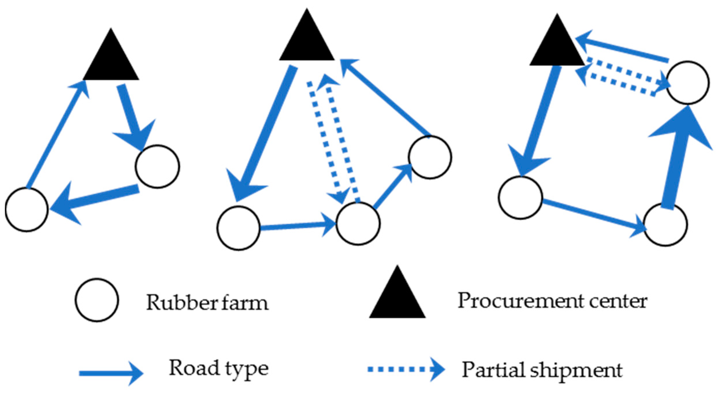
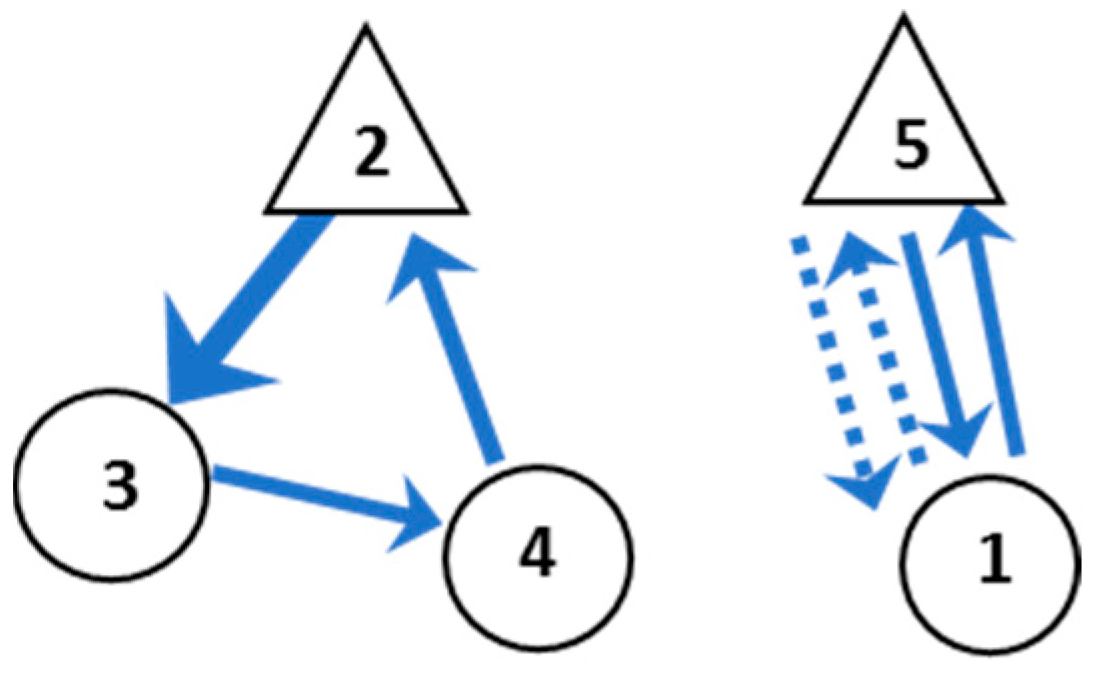
3.1. Problem Statement

This model aims to find the best location among all candidate rubber farms, then establish this location as the rubber procurement center. After that, the best transportation routes will be arranged for collecting rubber from farm to procurement center. The rubber quantity from each farm, capacity of the vehicle, and capacity of the procurement center are predefined parameters. The transportation road is different according to the road type, as indicated by different arrow sizes. The rubber farm is allowed to be served more than once by directed shipment (partial shipment), in case rubber quantity is over vehicle capacity, as indicated by the dotted lines. The problem statement is described in Figure 1.

This paper focuses on a case study of rubber logistics in southern Thailand. The case study contains 95 rubber farms. The road categories have been adopted from Akararungruangkul and Kaewman, 2018) [9]; divided into seven types based on average driving speed. The road type and fuel consumption rate are shown in

Table 1. Road categories and fuel consumption rates

Road Type	Ave. Speed (km/hr)	Fuel Consumption Rate (Liter/km)
A	30	0.118
B	40	0.107
C	50	0.112
D	60	0.090
E	70	0.098
F	80	0.098
G	90	0.102

.

Table 2. Road type metric of five farms

-	1	2	3	4	5
1	-	A	C	B	D
2	A	-	E	C	A
3	C	E	-	F	G
4	B	C	F	-	B
5	D	A	G	B	-

and

Table 3. Distance metric of five farms

-	1	2	3	4	5
1	-	21	43	41	27
2	21	-	32	35	28
3	43	32	-	46	30
4	41	35	46	-	22
5	27	28	30	22	-

illustrate the example of road type metric and distance metric for five rubber farms. Then, the fuel consumption metric can be calculated as shown in

Table 4. Fuel consumption metric of five farms

-	1	2	3	4	5
1	-	2.478	4.816	4.387	2.430
2	2.478	-	3.136	3.920	3.304
3	4.816	3.136	-	4.508	3.060
4	4.387	3.920	4.508	-	2.354
5	2.430	3.304	3.060	2.354	-

. The fuel consumption is calculated by multiplied fuel consumption rate and distance. This metric distinguishes our problem from the classical LRP which aims to optimize the travelling distance, as our model aims to minimize fuel consumption. Let us consider the following routes; 1-4-2-5-3-1 and 1-3-4-2-5-1. These routes have the total distance equal to 177 km and 179 km, but the fuel consumptions are 19.487 L and 18.978 L, respectively. Although route 1-3-4-2-5-1 is longer, our model will select this route for the reason of fuel minimization.

3.2. Mathematical Model

This study proposed a model that makes the decision of location routing design while considering environmental impact. The proposed model simultaneously determines the rubber procurement center locations and transportation routes with the objective function to minimize the fuel consumption costs of rubber collection. This combined approach manages location and vehicle routing plans at the same time. It is referred to in the literature surveys on LRPs [28,50]. The details of objective function, constraints, indices, parameters, decision variables, and support variables are shown below.

	Indices
	i	set of farms indexed by i and j
	Parameters
	Qi	Rubber quantity of farm i (kg)
	C	Fuel cost per liter (Baht)
	Dij	Distance from farm i to procurement center j (km)
	Fij	Fuel consumption rate from farm i to procurement center j
	V	Capacity of vehicle (kg)
	Pj	Capacity of procurement center (kg)
	Decision Variables
	zij	= 1 if farm i is assigned to procurement center j and direct shipment is appeared
		= 0 otherwise
	xij	= 1 if travel from farm i to farm j and routing for the rest of direct shipment is appeared
		= 0 otherwise
	ni	= Number of direct shipments at farm i
	Support Variables
	ui	Accumulated rubber quantity in vehicle at farm i for sub-tour elimination
	mj	Number of round travels of procurement center j
	ri	Remaining rubber after direct shipment from farm i
	yj	= 1 if procurement center j is chosen
		= 0 otherwise

Objective function

$$MinZ=C\left[{\displaystyle \sum }_{i\in I}{\displaystyle \sum }_{j\in I}{z}_{ij}{n}_i\left(D_{ij}{F}_{ij}\right)+{\displaystyle \sum }_{i\in I}{\displaystyle \sum }_{j\in I}{x}_{ij}{D}_{ij}{F}_{ij}\right]$$

(1)

Constraints

${\displaystyle \sum _{j\in I}}{z}_{ij}=1$	$\forall i\in I$	(2)
$Q_i=n_{i}V+r_i$	$\forall i\in I$	(3)
${\displaystyle \sum _{i\in I}}{z}_{ij}{Q}_i\le y_j{P}_j$	$\forall j\in I$	(4)
${\displaystyle \sum _{i\in I,i\ne j}}{x}_{ij}=\left(1-y_j\right)+y_j{m}_j$	$\forall j\in I$	(5)
${\displaystyle \sum _{j\in I,i\ne j}}{x}_{ij}={\displaystyle \sum _{j\in I,j\ne i}}{x}_{ji}$	$\forall i\in I$	(6)
$2x_{il}\le z_{ij}+z_{lj}+\left(1-z_{ij}\right)M$	$\forall i,j,l\in I,i\ne l$	(7)
$u_i+r_j\le u_j+V\left(1-x_{ij}\right)$	$\forall i,j\in I,i\ne j$	(8)
$r_i\le u_i\le V$	$\forall i\in I$	(9)
$x_{ij},z_{ij},y_j\in \left\{0,1\right\}$	$\forall i,j\in \left\{1,\dots M\right\}$	(10)

The mathematical model shown above can be described as following: (1) Is the objective function which is to minimize the total fuel consumption cost. The first term is direct shipment fuel cost, the second is routing fuel cost. Constraint (2) states that each farm must be assigned to only one procurement center. Constraint (3) determines the number of direct shipments and remaining rubber in case rubber quantity at the farm is over the capacity of vehicle. Constraint (4) ensures that total rubber at the procurement center must not exceed capacity. Constraint (5) determines the transportation route of rubber collection from the farm. Constraint (6) ensures that whenever the vehicle enters farm i, it must leave farm i. Constraint (7) provides the transportation route among the farms which are assigned to the same procurement center. Constraints (8) and (9) are capacity constraints related to vehicle capacity and sub-tour elimination. Finally, constraint (10) is a binary variable.

4. Solution Approach

This paper introduces the new metaheuristic-based method called variable neighborhood strategy adaptive search (VaNSAS), which is the new concept for solving combinatorial optimization problems. The elemental idea of the VaNSAS is to let the solution search for the better solution in a different area by using several searching methods. The searching method in VaNSAS can be a basic local search, well-known heuristics, modified metaheuristics, and a new designed local search, which is an advantage of VaNSAS that lets the designer put new ideas into the algorithm. Therefore, VaNSAS is very flexible to use for many optimization problems. Generally, the VaNSAS is composed of five steps which are: (1) generate a set of tracks; (2) all tracks select the specified black box; (3) execute the selected black box; (4) improve the track; and (5) repeat steps (1) to (4). The VaNSAS procedure can be explained as follows.

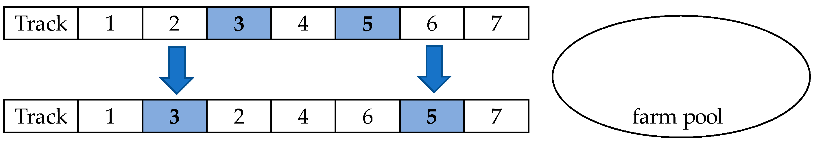
4.1. Generate a Set of Tracks

A track is the representative for the solution. A set of tracks is initially generated in terms of the real number. For example, if five tracks are generated and each track contains 15 elements, a set of tracks will be obtained as shown in

Table 5. Set of 5 random tracks

Track	1	2	3	4	5	6	7	8	9	10	11	12
1	0.77	0.31	0.46	0.43	0.15	0.57	0.65	0.05	0.24	0.52	0.86	0.75
2	0.02	0.92	0.39	0.31	0.44	0.16	0.41	0.35	0.45	0.44	0.38	0.28
3	0.82	0.92	0.14	0.22	0.62	0.66	0.96	0.59	0.36	0.08	0.44	0.11
4	0.86	0.94	0.02	0.43	0.9	0.14	0.27	0.52	0.47	0.4	0.83	0.45
5	0.76	0.57	0.39	0.65	0.06	0.93	0.31	0.02	0.54	0.98	0.51	0.25

. The number of tracks (NT) in each iteration is equal to five in this case—it is a predefined parameter that depends on designer decisions and problem size. Number of elements (NE) can be determined by equation 11, where NF is number of farm and NP is number of procurement centers. If the problem has five farms and two procurement center, then NE = 2(5)+2 = 12 elements.

$$NE=2NF+NP$$

(11)

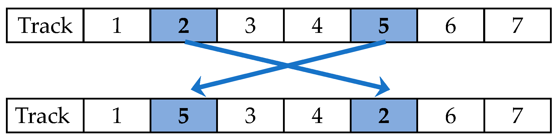
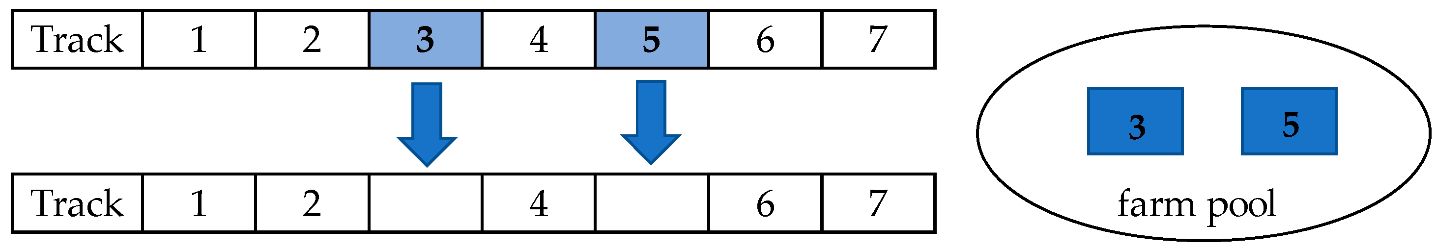
Track Interpretation Method

Track interpretation is the procedure that changes the code in each track to the solution of the problem. In order to illustrate the interpretation method, the related information is provided in

Table 6. Parameter used in track interpretation method

Item	Parameter
Procurement center	1	2
Capacity (kg)	25,000	25,000
Farm	1	2	3	4	5	Total
Rubber quantity (kg)	16,540	6970	5190	7450	2120	38,270
Vehicle capacity = 15,000 kg	Fuel cost = 28 baht/liter

. Let us consider five rubber farms with aggregate rubber of 38,270 kg, with the procurement centers chosen holding a capacity of 25,000 kg each. The number of procurement centers (NP) is set by aggregate rubber divided by 80% of their capacity, so in this problem, NP is equal to 2.

The track interpretation method can be explained by the following steps.

Step 1: Divide elements into three groups: A (depot or procurement center) = 5 elements, B (farm) = 5 elements and C (sequence) = 2 elements, as shown in

Table 7. Three groups of elements

Depot (A)					Farm (B)					Sequence (C)
1	2	3	4	5	1	2	3	4	5	1	2
0.77	0.31	0.46	0.43	0.15	0.57	0.65	0.05	0.24	0.52	0.86	0.75

. A sequence is used for setting the priority of a depot when assigning a farm to a depot.

Step 2: Sort the element value in each group by ascending order, as shown in

Table 8. Element values after sorting by each group

Depot (A)					Farm (B)					Sequence (C)
5	2	4	3	1	3	4	5	1	2	2	1
0.15	0.31	0.43	0.46	0.77	0.05	0.24	0.52	0.57	0.65	0.75	0.86

.

Step 3: Group A: select the first two numbers (NP = 2) to be the procurement center, so farm 5 and farm 2 will be depots.

Group C: The sequence is 2 and 1; this means depot 2 is the first priority to assign, so start assigning a farm to depot 2, then to depot 5.

Step 4: Group B: start assigning farm 3 and farm 4 to depot 2 until it satisfies the capacity constraint. The total rubber is farm 2 (depot) + farm 3 + farm 4 = 19,160 kg, but the vehicle load is farm 3 + farm 4 = 12,640 kg. Then, the assignment will be stopped and depot 5 will be started. The next number is farm 1, so assign it to depot 5. The partial shipment occurs in farm 1 because it has more rubber than vehicle capacity. The next number is farm 2, but it is skipped because it has been selected to be a depot already.

This step will allow the initial solution to always obtain feasible state because the assignment method will satisfy the constraint of vehicle capacity and depot capacity at all iterations.

From Figure 2, farm 1 will be visited twice according to our special constraint. The objective function will be calculated by using fuel consumption data given in Table 4. For route 2-3-4-2, the fuel consumption cost is (3.136 + 4.508 + 3.920) × 28 = 323.792 baht. For route 5-1-5-1-5, (2.430 × 2 × 2) × 28 = 272.160 baht. Thus, the total fuel consumption of this track is 323.792 + 272.160 = 595.952 baht.

4.2. All Tracks Select the Specified Black Box

Black box is the algorithm that is designed to improve the solution. This step allows the tracks obtained from previous step to improve themselves by selecting to enter in a black box. The black box methods and the black box numbers are unrestricted. It can be a simple local search or well-known heuristics or any metaheuristics, such as genetic algorithm (GA), simulated annealing (SA), and particle swarm optimization (PSO). It is based on the designer’s decision and the complexity of the problem. In each iteration, a track will randomly select the preferred black box. This step means that a single solution can change the neighborhood at any the time. The selection of a black box will be performed using the probability in Equations (12)–(13).

$$P_{bt}=F{N}_{bt-1}+\left(1-F\right)A_{bt-1}+K{I}_{bt-1}+M{Z}_{bt-1}$$

(12)

$$P_{bt}=F{N}_{bt-1}+\left(1-F\right)A_{bt-1}+K{I}_{bt-1}$$

(13)

where P_bt is probability of selecting black box b in iteration t. I_bt-1 is a bonus point; it is given 1 point if the black box of the last iteration contains the best solution, but given zero if this is not the case. A_bt-1 is the average objective value of every track which selects black box b in the last iteration. N_bt-1 is the number of tracks that select black box b in the last t iteration. Z_bt-1 is the best objective obtained from black box b in the last iteration. F, K, and M are predefined parameters.

4.3. Execute the Selected Black Box

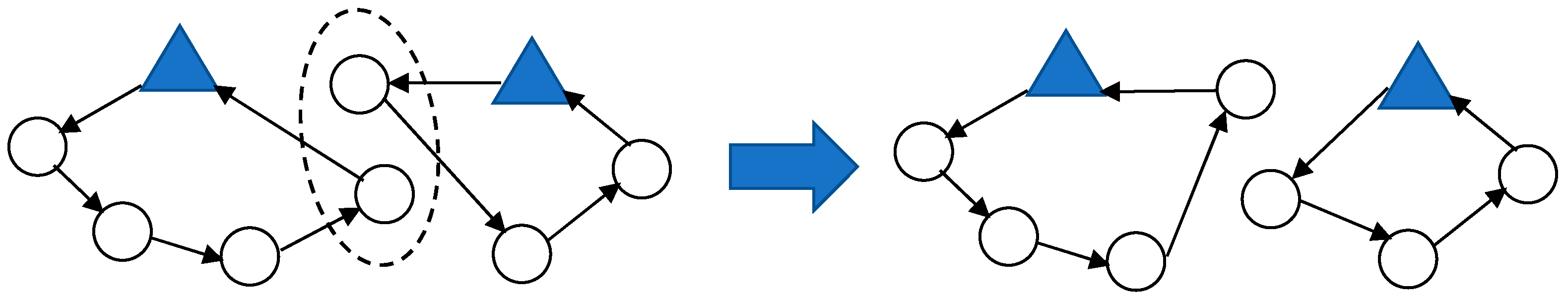
This paper proposes that three black boxes contain three algorithms which are (1) SWAP heuristic; (2) adaptive large neighborhood search (ALNS); and (3) variable neighborhood search (VNS). The procedure of these algorithms will be revealed as follows.

4.3.1. SWAP

SWAP is the simple and basic local search method. Searching moves positions one-by-one until it covers all positions. A SWAP operator in this paper consists of two indices (a, b), which were applied to the initial solution to obtain a new solution. For example, if an initial solution is S = (1-2-3-4-5-6-7), (a, b) = (2, 5); then a new solution is S’ = (1-5-3-4-2-6-7). The procedure of SWAP shows as the following steps.

Step 1: Initial solution obtained from the track that chooses to operate in this black box.

Step 2: Randomly select two indices (a, b) = (farm 2, farm 5), then exchange their position. Example of SWAP is illustrated in Figure 3.

Step 3: Perform interpretation process of a track.

Step 4: Repeat step 2 to 4 until all positions have been exchanged.

Step 5: Return the best solution.

4.3.2. Adaptive Large Neighborhood Search (ALNS)

ALNS consists of a destroying and a repairing operation; each operation contains a set of destroying and repairing methods called operators. The operator will be assigned a weight which is adjusted in every iteration based on its success. The weight reflects the operator’s performance and the selection of an operator in each iteration is based on its weight. The operator which has a high performance will have more chance to be selected repeatedly. The procedure of ALNS shows as the following steps.

Step 1: Initial solution obtained from the track that chooses to operate in this black box; let it be s.

Step 2: Setting the initial solution s is the best solution s*.

Step 3: Setting the weight and selected probability of each operator.

Step 4: Randomly select destroying and repairing operators according to their weight.

Step 5: Apply the operators to the current solution, then a new solution (s’) will be obtained.

Step 6: Perform interpretation process of a track.

Step 7: Perform acceptance criterion.

If the acceptance criterion is met, then s ← s’.

If s is better than s*, then s* ← s’.

Step 8: Adjust weight.

Step 9: Repeat step 3 to 8 until stopping criterion is met.

Step 10: Return the best solution.

The acceptance criterion in Step 7 is performed for accepting or rejecting a new solution (s’). This paper uses a greedy acceptance principle which only accept s’, if it is better than the current solution (s).

This paper designs three destroying operators and two repairing operators which will be explained in the below section.

Destroying Operators

Destroying operators are used to remove a part of the current solution. Degree of removal (d) is randomly selected in each iteration by varying amounts, from 10% to 40% of farms, representing light removal to strong removal. After selection of d, the q farms will then be removed from the current solution. An example of the destroying operation is shown in Figure 4.

• Random Removal

This operator randomly removes q farms from the initial solution.

Step 1: Randomly choose degree of removal, let d = 30%. If the initial solution contains seven farms, two farms will be removed.

Step 2: Remove those farms to the farm pool.

• Worst Removal

This operator removes the worst farm that generates the highest cost in the initial solution.

Step 1: Randomly choose degree of removal, let d = 30%. If the initial solution contains seven farms, two farms will be removed.

Step 2: Calculate the total cost of the initial solution.

Step 3: Remove farm one by one from the initial solution, then calculate the different value by comparing it to the total cost of the initial solution.

Step 4: Ranking farm by decreasing order based on different values in Step 3.

Step 5: Remove the first two farms which have large values to the farm pool.

• Related Removal

Step 1: Randomly choose degree of removal, let d = 30%. If the initial solution contains seven farms, two farms will be removed.

Step 2: Randomly choose a farm, called a seed farm.

Step 3: Calculate the value of total cost when traveling from the seed farm to each farm.

Step 3: Ranking farms by descending order based on values in Step 3.

Step 4: Remove q–1 farms which have the least value to the farm pool.

Repairing Operators

When a destroying operator is executed, then a repairing operator is applied to re-insert the farms in different positions by expecting the better solution. An example of repairing operation is shown in Figure 5.

• Random Insertion

The farms from the farm pool will be randomly inserted back to the solution.

• Best Insertion

The algorithm will search the best position by considering the minimal total cost.

Step 1: Determine a position to insert a farm, then calculate the total cost.

Step 2: Insert a farm into the lowest total cost position.

Step 3: Re-do step 1 and step 2 until all farms in the farm pool are inserted.

4.3.3. Variable Neighborhood Search (VNS)

Three different neighborhood structures are defined, N = {N₁, N₂, N₃}

• Farms Exchange (N₁)

A neighbor of a solution S of N₁ is acquired by exchanging two random farms from the same route or same depot, from the different route or a different depot. Example of a farm’s exchange structure is shown in Figure 6.

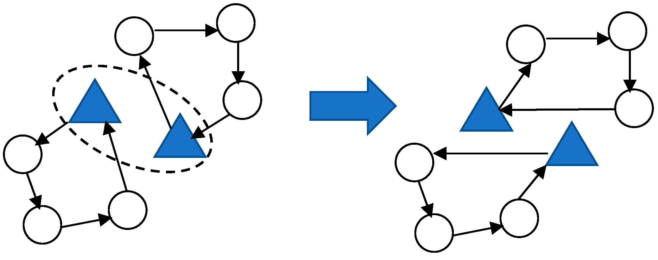
• Depots Exchange (N₂)

A neighbor of a solution S of N₂ is acquired by exchanging the farms between two random depots. All farms in a depot will be re-assigned to another depot by exchanging each other. An example of a depot exchange structure is shown in Figure 7.

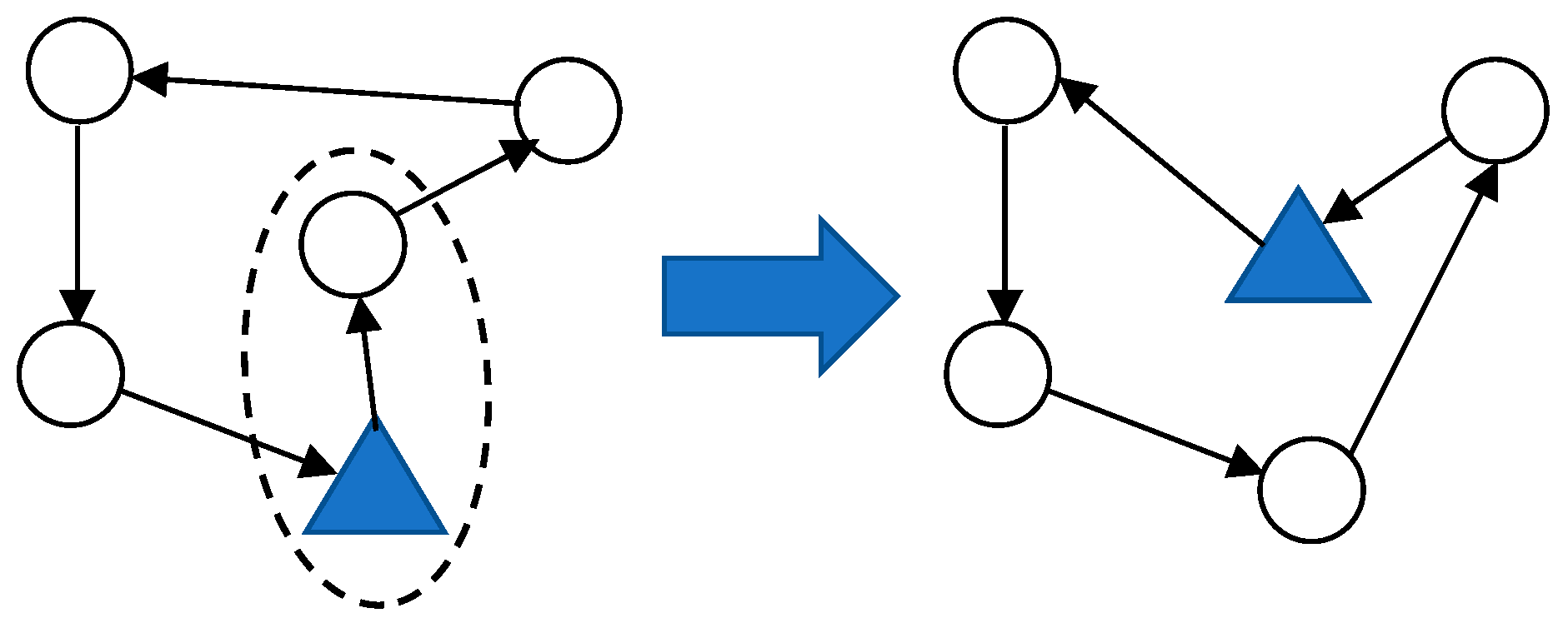
• Depot Status Change (N₃)

A neighbor of a solution S of N₃ is acquired by closing an open depot and opening another one, then re-assigning all farms to the new depot. An example of a depot status change structure is shown in Figure 8.

VNS algorithm is summarized in Algorithm 1. The neighborhood structures (N₁–N₃) are randomly selected during k iteration.

Algorithm 1 VNS

Input: Set of neighborhood structures N = {N1, N2, N3} Initialization: Initial solution (a track that chooses to operate in this black box) = s kmax = 10 repeat   k ← 1   while k ≤ kmax do      s’ ← select (N1, N2, N3)      s’’ ← local search s’      if f(s’’) < f(s) then        s ← s’’         k ← 1      else        k ← k+1     end if    end while until stopping criterion is met return s

4.4. Improve the Track

Equations (14)–(15) are used to improve all information in the track.

$$Z_{ijt+1}=Z_{ijt}+\alpha \left(Z_{ijt}^{pb}-Z_{ijt}\right)+\left(1-\alpha \right)\left(Z_{ijt}^{gb}-Z_{ijt}\right)+\beta \left(Z_{2jt}-Z_{3jt}\right)$$

(14)

$$Z_{ijt+1}=Z_{ijt}+\alpha \left(Z_{ijt}^{pb}-Z_{ijt}\right)+\left(1-\alpha \right)\left(Z_{ijt}^{gb}-Z_{ijt}\right)$$

(15)

where $Z_{ijt+1}$ is track i, element j at iteration t + 1. $Z_{ijt}$ is track i, element j at the last iteration. $\alpha$ and $\beta$ are predefined parameters. $Z_{2jt}$ is the first randomly selected track and $Z_{3jt}$ is the second randomly selected track. $Z_{ijt}^{pb}$ is the personal best track and $Z_{ijt}^{gb}$ is the global best track.

4.5. Repeat Step 1 to 4

Repeat steps 2 to 4 iteratively.

VaNSAS is the new type of metaheuristics for which the target is to let algorithms search in many different areas to obtain the best solution possible. The searching can move to have more diversification and intensification at all times depending on the black box methods that are designed to use. The VaNSAS algorithm is shown in Algorithm 2.

Algorithm 2 VaNSAS

Input Number of farms, fuel consumption rate, distance, rubber quantity, related capacity Output Fuel cost Begin While I less than predefined number of iterations.       1. Randomly generate number of track (NT) Zijt       2. Each track individually choses black box       3. Operate black box            (optional) SWAP            (optional) ALNS            (optional) VNS       4. Improve the track        I = I + 1; End

5. Computational Framework and Result

The proposed heuristic has been tested with three groups of testing instances. Group 1: small-sized cases, contains five to nine rubber farms. Group 2: medium-sized cases, contains 10–30 rubber farms. Group 3: medium-sized cases, contains 35–50 rubber farms and the case study problem. The computational framework is shown in

Table 9. Details of the test instances

Instance	Number of Farms	Total Rubber (kg)	Instance	Number of Farms	Total Rubber (kg)	Instance	Number of Farms	Total Rubber (kg)
S1	5	18,667	M1	20	42,856	L1	35	83,176
S2	6	25,241	M2	20	48,665	L2	40	87,368
S3	7	27,353	M3	25	58,993	L3	40	88,842
S4	8	28,535	M4	25	58,250	L4	45	92,254
S5	9	33,518	M5	30	78,665	L5	50	96,697
						Case study	95	204,427

. The complexity of the problem instances is explained as follows. The number of constraints and decision variables of Group 1 are 255–1,107 and 55–171 respectively. The number of constraints and decision variables of Group 2 are 9,720–30,780 and 820–1,830 respectively. The number of constraints and decision variables of Group 3 are 47,985–894,045 and 2,485–18,145 respectively.

All proposed algorithms have been compared with the solutions obtained from Lingo v.11 software. The lower bound was compared in case the optimal solution was not obtainable within limited time. The heuristics were tested for five runs, then the best solution reported among the five runs. Each method was set a number of iterations with 1000 as the stopping criterion. The mathematical model and the proposed algorithms were coded by Visual studio 2019 on PC Intel Core i5 CPU 2.70 GHz Ram 4 GB operated on Window 8.1 Pro. All statistical tests were conducted at the 95% confidence level.

The algorithm consists of two methods of black box selection and track improvement. The combinations of the proposed algorithms are defined, as detailed in

Table 10. Name of the proposed algorithms

Algorithms Name	Definition
VaNSAS-1	Using black box selection equation (12) + track improvement equation (14)
VaNSAS-2	Using black box selection equation (12) + track improvement equation (15)
VaNSAS-3	Using black box selection equation (13) + track improvement equation (14)
VaNSAS-4	Using black box selection equation (13) + track improvement equation (15)

.

In order to assess the value of parameters, the DOE method of factorial design was used via Minitab software (Minitab Inc.). Figure 9 shows the optimization plot result, the value of parameters which are used in the proposed algorithms are shown as follow: F = 0.90, K = 0.10, M = 0.90, α = 0.90 and β = 0.90.

Table 11. Computational results of testing instances

Instances	Lingo			VaNSAS-1		VaNSAS-2		VaNSAS-3		VaNSAS-4
	Status	Objective (Baht)	Time (mins)	Objective (Baht)	Time (mins)	Objective (Baht)	Time (mins)	Objective (Baht)	Time (mins)	Objective (Baht)	Time (mins)
SM1	Glo.opt *	269.09	0.11	269.09	0.24	269.09	0.25	269.09	0.21	269.09	0.16
SM2	Glo.opt	430.62	0.15	430.62	0.26	430.62	0.22	430.62	0.23	430.62	0.20
SM3	Glo.opt	369.16	0.13	369.16	0.28	369.16	0.26	369.16	0.35	369.16	0.26
SM4	Glo.opt	315.68	0.14	315.68	0.34	315.68	0.21	315.68	0.31	315.68	0.28
SM5	Glo.opt	418.27	0.16	418.27	0.32	418.27	0.25	418.27	0.37	418.27	0.25
Average		360.56	0.14	360.56	0.29	360.56	0.24	360.56	0.29	360.56	0.23
ME1	BOF **	2116.77	2880	2087.23	2.43	2087.23	2.56	2087.23	2.21	2087.23	2.38
ME2	BOF	2135.97	2880	2082.65	2.12	2082.65	2.38	2082.65	1.87	2082.65	1.93
ME3	BOF	2367.63	2880	2276.28	2.54	2260.21	2.76	2282.26	1.93	2282.26	2.06
ME4	BOF	2471.43	2880	2387.05	2.69	2404.44	2.62	2404.44	2.41	2407.33	2.52
ME5	BOF	2843.99	2880	2741.47	2.73	2745.62	2.69	2795.52	2.56	2741.47	2.45
Average		2387.16	2880.00	2314.94	2.50	2316.03	2.60	2330.42	2.20	2320.19	2.27
LA1	Bound ***	3885.37	7200	4214.33	7.32	4214.33	7.61	4312.25	8.02	4214.33	8.22
LA2	Bound	4322.43	7200	4698.34	8.19	4725.87	7.43	4791.33	7.84	4725.87	7.65
LA3	Bound	4569.53	7200	4889.22	8.24	4902.33	7.75	4910.85	7.86	4889.22	8.15
LA4	Bound	4869.86	7200	5123.55	8.15	5221.76	7.62	5233.51	8.24	5123.55	8.41
LA5	Bound	5288.90	7200	5592.08	9.21	5603.41	8.39	5605.38	9.15	5603.41	9.35
Case study	Bound	10,772.45	7200	13,280.45	18.16	13,343.28	16.76	13,838.54	17.31	13,322.88	18.44
Average		5618.09	7200.00	6299.66	9.88	6335.16	9.26	6448.64	9.74	6313.21	10.04

* Glo.opt = Global optimal solution, ** BOF = Best solution found during limited time, *** Bound = Lower bound.

shows the testing results of all sized instances. For small-sized instances, both Lingo and proposed algorithms could find the optimal solutions within short computational times. Because the problems were small, the difference was not obvious.

For medium-sized instances, Lingo could not find the optimal solutions within a computational time of 48 h, the solutions were only the best it could find during the time restriction. On the other hand, proposed algorithms could find the better solution within shorter computational time.

Table 12. Percentage gap of proposed heuristics and results from Lingo

Instance	VaNSAS-1	VaNSAS-2	VaNSAS-3	VaNSAS-4
SM1	0.00	0.00	0.00	0.00
SM2	0.00	0.00	0.00	0.00
SM3	0.00	0.00	0.00	0.00
SM4	0.00	0.00	0.00	0.00
SM5	0.00	0.00	0.00	0.00
Average	0.00	0.00	0.00	0.00
ME1	−1.42	−1.42	−1.42	−1.42
ME2	−2.56	−2.56	−2.56	−2.56
ME3	−4.01	−4.75	−3.74	−3.74
ME4	−3.53	−2.79	−2.79	−2.66
ME5	−3.74	−3.58	−1.73	−3.74
Average	−3.05	−3.02	−2.45	−2.82
LA1	7.81	7.81	9.90	7.81
LA2	8.00	8.54	9.79	8.54
LA3	6.54	6.79	6.95	6.54
LA4	4.95	6.74	6.95	4.95
LA5	5.42	5.61	5.65	5.61
Case study	18.88	19.27	22.16	19.14
Average	8.60	9.13	10.23	8.76

illustrates percentage gap between two methods that calculated solutions using equation 16. The proposed VaNSAS obtained the percentage gap of 3.05%, 3.02%, 2.45%, and 2.82%, respectively. The statistical test in

Table 13. Statistical results of medium-sized instances

Method	VaNSAS-1	VaNSAS-2	VaNSAS-3	VaNSAS-4
Lingo	0.006	0.008	0.004	0.006
VaNSAS-1	-	0.848	0.202	0.253
VaNSAS-2	-	-	0.218	0.418
VaNSAS-3	-	-	-	0.404

shows that all proposed VaNSAS perform significantly differently from Lingo’s solution and all VaNSAS are non-significantly different from each other. Besides, the computational time of VaNSAS outperformed Lingo, consuming an average time of only 2.5 min, 2.6 min, 2.2 min, and 2.27 min, respectively.

$$\%gap=\left(\frac{S_P-S_L}{S_P}\right)\times 100\%$$

(16)

where $\%gap$ is the percentage difference between Lingo and VaNSAS, $S_P$ is the solution obtained from the proposed VaNSAS, and $S_L$ is the solution obtained from Lingo.

For large-sized instances, Lingo used 120 h to find the solutions, but it could find only lower bound. However, the VaNSAS used only 9–10 min to find the reasonable solutions. Although these solutions may not be optimal, the statistical test in

Table 14. Statistical results of large-sized instances

Method	VaNSAS-1	VaNSAS-2	VaNSAS-3	VaNSAS-4
Lingo	0.121	0.111	0.123	0.120
VaNSAS-1	-	0.069	0.135	0.121
VaNSAS-2	-	-	0.205	0.219
VaNSAS-3	-	-	-	0.143

reveals that there is a non-significant difference between Lingo’s solutions and VaNSAS’s solutions. Moreover, all VaNSAS are non-significantly different from each other in solving the large problem.

The percentage gap results in Table 12 were analyzed by using the ANOVA method to validate whether VaNSAS executed differently when the problem size was larger. The testing results are shown in

Table 15. ANOVA test to validate the impact of the problem size to the efficiency of algorithms

	VaNSAS-1	VaNSAS-2	VaNSAS-3	VaNSAS-4
p-value	0.001	0.001	0.001	0.001

.

From Table 15, when the problem size was larger, all proposed VaNSAS performed significantly differently from Lingo’s solutions. Nevertheless, the statistical results indicated that the solutions from VaNSAS were non-significantly different from Lingo’s solutions in small-sized and large-sized instances. Furthermore, the VaNSAS obtained the better results than Lingo in medium-sized instances within limited time.

VaNSAS-1 showed the best performance when considered percentage gap in all sized instances. Therefore, this approach has been implemented to the case study problem and

Table 16. Case study result from VaNSAS-1

No.	Selected Location	Transportation Route	Distance (km)	Fuel Used (liter)	Fuel Cost (Baht)
1	45	45-91-92-89-87-86-88-32-35-34-33-24-25-38-45	508.31	50.27	1407.56
2		45-42-43-37-26-45	249.77	21.92	613.88
3	36	36-84-81-83-82-85-55-36	480.02	42.92	1201.72
4	15	15-16-15	80.70	7.26	203.28
5		15-13-44-15	112.13	8.72	244.28
6	77	77-75-52-11-94-73-80-77	287.92	28.01	784.16
7		77-54-51-70-79-77	119.49	10.04	281.00
8		77-64-65-66-67-77	49.71	4.18	117.12
9		77-78-77	64.06	6.28	175.89
10	1	1-4-1	86.96	7.81	218.56
11		1-4-7-1	108.58	11.09	310.52
12		1-39-93 -1	167.03	16.89	472.88
13	76	76-53-6-5-76	231.82	22.44	628.32
14		76-59-60-61-62-63-69-72-71-68-74-76	619.42	60.78	1701.96
15	17	17-41-40-90-17	392.69	38.46	1076.88
16		17-23-27-30-28-31-29-17	358.06	32.14	899.84
17		17-19-3-8-9-17	219.55	21.05	589.40
18	10	10-20-22-21-10	202.66	18.47	517.20
19		10-18-14-12-2-10	198.99	18.02	504.60
20	49	49-47-49	107.56	10.54	295.12
21		49-46-50-48-47-49	175.79	16.55	463.40
22		49-56-57-58-95-49	210.37	20.46	572.88
		Total	5031.59	474.30	13,280.45

shows the results of the case study. There are nine procurement centers which buy and collect the rubber from all farms across 22 transportation routes. The total fuel consumption cost is minimized to 13,280.45 baht. The special constraint that a farm can be visited more than once was applied in route nos. 10 and 20; farm nos. 4 and 47 were visited twice because they had more rubber than the vehicle’s capacity.

The last experiment was conducted to show VaNSAS-1 performance by verifying the solution plot in Figure 10. The main idea of VaNSAS was to let the algorithm constantly change the searching area by applying diversification and intensification concepts. It can escape from the trap of local optima, then move to other areas, as implied by the turning point of the graph line. Therefore, VaNSAS can find often the new optimal solution, it can find new best solution during the all simulation time.

6. Conclusions and Future Research

This research has presented a new solution approach for solving location routing problems in agricultural logistics. The problem contained two main stages: (1) the selection of rubber procurement locations, and (2) the routing management of rubber collection. In this problem, the farm could generate more rubber than the vehicle’s capacity, so this paper added the special constraint of letting the farm be visited more than once. The mathematical model has been formulated to represent the case study problem with the objective function to minimize the total fuel consumption cost.

The heuristic proposed in this research was called the variable neighborhood strategy adaptive search (VaNSAS). The VaNSAS comprised of three searching strategies which were: (1) swap, (2) adaptive large neighborhood search (ALNS), and (3) variable neighborhood search (VNS). These strategies were selected randomly to improve solutions in each searing iteration. Furthermore, we split the proposed heuristic into four sub-heuristics; VaNSAS-1, VaNSAS-2, VaNSAS-3, and VaNSAS-4, to evaluate the performance of the black box selection formula and track improvement formula.

The computational result showed that VaNSAS-1 outperformed the other proposed heuristics because it obtained the smallest gap when compared to Lingo’s results. This implied the mixing of black box selection Formula 12 and track improvement Formula 14. Formula 12 selected a black box based on the intensification concept because it included a weighting of the best objective obtained from the black box. Thus, the best black box in the last iteration had more chance to be selected repeatedly. Formula 14 improved track information based on the diversification concept since it combined with the two random track’s information to create the new track. Therefore, VaNSAS-1 has been selected to solve the case study problem. The results shown that nine farms were selected to be rubber procurement centers and 22 transportation routes were designed with the lowest total fuel cost. The computational experiment indicates that the new optimization technique can solve this case study problem effectively. The solution shows several farms were served twice according to the special constraint. These results describe the contributions of this research.

Akararungruangkul and Kaewman [9] applied modified differential evolution (MDE) for special case of LRP with fuel used minimization. For case study problem which contain 110 farms, the proposed MDE can save 15.05% of fuel amount comparing to current practice. The extended experiment of VaNSAS-1 reveals that 5.48% of fuel cost can be saved from traditional LRP. However, the problem size and the case problem are different. The larger the problem is, the greater savings it can obtain. The different distancesin different cases effect the comparison of both studies as well.

This paper based on static supply assumption; the rubber quantity of each farm is predefined number acquired from historical data. This is the limitation because the location and routing plan may not be suitable when the rubber quantity is changed. Besides, the data collection needs to be prompt and update in real-time. For future research, the authors suggest that another real-world constraint should be considered, such as stochastic supply according to daily rubber tapping of farmers. This will affect the selection of procurement center locations and routing paths as a daily dynamic move. A mobile application could be developed to support the gathering of daily rubber amounts from each farm, and the data will be sent for processing via a proposed algorithm to obtain the suitable procurement center locations and routes. Another suggestion is to apply VaNSAS to other optimization problems, allowing this algorithm to be opened for innovation in other industries and organizations.

References

1. Marchiol, L. An Outlook of Crop Nutrition in the Fourth Agricultural Revolution. Ital. J. Agron. 2019, 14, 1367. [Google Scholar] [CrossRef]
2. Sung, J. The Fourth Industrial Revolution and Precision Agriculture. In Automation in Agriculture: Securing Food Supplies for Future Generations; IntechOpen: London, UK, 2018. [Google Scholar]
3. Bank of Thailand. Major Agricultural Price in Thailand Report. 2019. Available online: https://www.bot.or.th/Thai/MonetaryPolicy/NorthEastern/Pages/commodities.aspx (accessed on 9 September 2019).
4. The Board of Investment of Thailand. Thailand’s Rubber Industry. Available online: https://www.boi.go.th/upload/content/Rubber_5a3b80bcc4882.pdf (accessed on 2 November 2019).
5. Trade Statistics for International Business Development. List of Exporters for the Selected Product in 2018. Available online: https://www.trademap.org/Country_SelProduct.aspx?nvpm=1%7c%7c%7c%7c%7c4001%7c%7c%7c4%7c1%7c1%7c2%7c1%7c1%7c2%7c1%7c1 (accessed on 2 November 2019).
6. The Board of Investment of Thailand: world’s Top Supplier of Natural Rubber. Available online: https://www.boi.go.th/upload/content/Rubber_Industry2018_5bb33471b8292.pdf (accessed on 2 November 2019).
7. Lee, D. Thailand Natural Rubber Economics. Available online: https://www.halcyonagri.com/thailand-natural-rubber-economics (accessed on 2 November 2019).
8. Srisawadi, S.; Paoprasert, N.; Wattanawongsakun, P.; Lerspalungsanti, S.; Srisurangkul, C.; Pitaksapsin, N. Cost and Benefit Analysis for Rubber Product Transportation. In Proceedings of the 4th International Conference on Engineering, Project, and Production Management (EPPM 2013), Bangkok, Thailand, 23–25 October 2013; pp. 450–459. [Google Scholar]
9. Akararungruangkul, R.; Kaewman, S. Modified Differential Evolution Algorithm Solving the Special Case of Location Routing Problem. Math. Comput. Appl. 2018, 23, 34. [Google Scholar] [CrossRef] [Green Version]
10. Larson, P. Designing and Managing the Supply Chain: Concepts, Strategies, and Case Studies, David Simchi-Levi Philip Kaminsky Edith Simchi-Levi. J. Bus. Logist. 2001, 22, 259. [Google Scholar] [CrossRef]
11. Watson-Gandy, C.D.T.; Dohrn, P.J. Depot location with van salesmen—A practical approach. Omega 1973, 1, 321–329. [Google Scholar] [CrossRef]
12. Madsen, O.B.G. Methods for solving combined two level location-routing problems of realistic dimensions. Eur. J. Oper. Res. 1983, 12, 295–301. [Google Scholar] [CrossRef]
13. Alumur, S.; Kara, B.Y. A new model for the hazardous waste location-routing problem. Comput. Oper. Res. 2007, 34, 1406–1423. [Google Scholar] [CrossRef] [Green Version]
14. Schiffer, M.; Walther, G. The electric location routing problem with time windows and partial recharging. Eur. J. Oper. Res. 2017, 260, 995–1013. [Google Scholar] [CrossRef]
15. Yakıcı, E. Solving location and routing problem for UAVs. Comput. Ind. Eng. 2016, 102, 294–301. [Google Scholar] [CrossRef]
16. Wang, X.; Li, X. Carbon reduction in the location routing problem with heterogeneous fleet, simultaneous pickup-delivery and time windows. Procedia. Comput. Sci. 2017, 112, 1131–1140. [Google Scholar] [CrossRef]
17. Demir, E.; Bektaş, T.; Laporte, G. A review of recent research on green road freight transportation. Eur. J. Oper. Res. 2014, 237, 775–793. [Google Scholar] [CrossRef] [Green Version]
18. Karaoglan, I.; Altiparmak, F.; Kara, I.; Dengiz, B. A branch and cut algorithm for the location-routing problem with simultaneous pickup and delivery. Eur. J. Oper. Res. 2011, 211, 318–332. [Google Scholar] [CrossRef]
19. Albareda-Sambola, M.; Fernández, E.; Nickel, S. Multiperiod location-routing with decoupled time scales. Eur. J. Oper. Res. 2012, 217, 248–258. [Google Scholar] [CrossRef]
20. Samanlioglu, F. A multi-objective mathematical model for the industrial hazardous waste location-routing problem. Eur. J. Oper. Res. 2013, 226, 332–340. [Google Scholar] [CrossRef]
21. Vincent, F.Y.; Lin, S.-Y. A simulated annealing heuristic for the open location-routing problem. Comput. Oper. Res. 2015, 62, 184–196. [Google Scholar]
22. Toro, E.M.; Franco, J.F.; Echeverri, M.G.; Guimarães, F.G. A multi-objective model for the green capacitated location-routing problem considering environmental impact. Comput. Ind. Eng. 2017, 110, 114–125. [Google Scholar] [CrossRef] [Green Version]
23. Govindan, K.; Jafarian, A.; Khodaverdi, R.; Devika, K. Two-echelon multiple-vehicle location–routing problem with time windows for optimization of sustainable supply chain network of perishable food. Int. J. Prof. Econ. 2014, 152, 9–28. [Google Scholar] [CrossRef]
24. Dukkanci, O.; Peker, M.; Kara, B.Y. Green hub location problem. Transp. Res. Part F Log. Transp. 2019, 125, 116–139. [Google Scholar] [CrossRef]
25. Dukkanci, O.; Kara, B.Y.; Bektaş, T. The green location-routing problem. Comput. Oper. Res. 2019, 105, 187–202. [Google Scholar] [CrossRef]
26. Toro, E.; Franco, J.; Granada-Echeverri, M.; Guimarães, F.; Rendón, R. Green open location-routing problem considering economic and environmental costs. Int. J. Ind. Eng. Comput. 2016, 8, 203–216. [Google Scholar] [CrossRef]
27. Wang, S.; Tao, F.; Shi, Y. Optimization of Location–Routing Problem for Cold Chain Logistics Considering Carbon Footprint. Int. J. Environ. Res. Public Health. 2018, 15, 86. [Google Scholar] [CrossRef] [Green Version]
28. Nagy, G.; Salhi, S. Location-routing: Issues, models and methods. Eur. J. Oper. Res. 2007, 177, 649–672. [Google Scholar] [CrossRef] [Green Version]
29. De, A.; Mogale, D.G.; Zhang, M.; Pratap, S.; Kumar, S.K.; Huang, G.Q. Multi-period multi-echelon inventory transportation problem considering stakeholders behavioural tendencies. Int. J. Prod. Econ. 2019, 107566. [Google Scholar] [CrossRef]
30. De, A.; Choudhary, A.; Turkay, M.K.; Tiwari, M. Bunkering policies for a fuel bunker management problem for liner shipping networks. Eur. J. Oper. Res. 2019. [Google Scholar] [CrossRef]
31. Barreto, S.; Ferreira, C.; Paixão, J.; Santos, B.S. Using clustering analysis in a capacitated location-routing problem. Eur. J. Oper. Res. 2007, 179, 968–977. [Google Scholar] [CrossRef]
32. Boudahri, F.; Mtalaa, W.; Bennekrouf, M.; Sari, Z. Application of a Clustering Based Location-Routing Model to a Real Agri-food Supply Chain Redesign. In Advanced Methods for Computational Collective intelligence; Springer: Berlin/Heidelberg, Germany, 2013; Volume 457, pp. 323–331. [Google Scholar]
33. Yu, V.F.; Lin, S.-W.; Lee, W.; Ting, C.-J. A simulated annealing heuristic for the capacitated location routing problem. Comput. Ind. Eng. 2010, 58, 288–299. [Google Scholar] [CrossRef]
34. Sajjadi, S.R.; Cheraghi, S. Multi-products location-routing problem integrated with inventory under stochastic demand. Int. J. Ind. Syst. Eng. 2011, 7, 454–476. [Google Scholar] [CrossRef]
35. Karaoglan, I.; Altiparmak, F.; Kara, I.; Dengiz, B. The location-routing problem with simultaneous pickup and delivery: Formulations and a heuristic approach. Omega 2012, 40, 465–477. [Google Scholar] [CrossRef]
36. Stenger, A.; Schneider, M.; Schwind, M.; Vigo, D. Location routing for small package shippers with subcontracting options. Int. J. Pro. Econ. 2012, 140, 702–712. [Google Scholar] [CrossRef]
37. Derbel, H.; Jarboui, B.; Hanafi, S.; Chabchoub, H. An Iterated Local Search for Solving a Location-Routing Problem. Electron. Notes. Discret. Math. 2010, 36, 875–882. [Google Scholar] [CrossRef]
38. De, A.; Wang, J.; Tiwari, M.K. Fuel Bunker Management Strategies within Sustainable Container Shipping Operation Considering Disruption and Recovery Policies. IEEE Trans. Eng. Manag. 2019, 1–23. [Google Scholar] [CrossRef] [Green Version]
39. De, A.; Wang, J.; Tiwari, M. Hybridizing Basic Variable Neighborhood Search With Particle Swarm Optimization for Solving Sustainable Ship Routing and Bunker Management Problem. IEEE Trans. Intell. Transp. Syst. 2019, 1–12. [Google Scholar] [CrossRef]
40. Mladenović, N.; Hansen, P. Variable neighborhood search. Comput. Oper. Res. 1997, 24, 1097–1100. [Google Scholar] [CrossRef]
41. Jarboui, B.; Derbel, H.; Hanafi, S.; Mladenović, N. Variable neighborhood search for location routing. Comput. Oper. Res. 2013, 40, 47–57. [Google Scholar] [CrossRef]
42. Schwengerer, M.; Pirkwieser, S.; Raidl, G. A Variable Neighborhood Search Approach for the Two-Echelon Location-Routing Problem; Springer: Berlin/Heidelberg, Germany, 2012; Volume 7245, pp. 13–24. [Google Scholar]
43. Macedo, R.; Hanafi, S.; Jarboui, B.; Mladenovic, N.; Alves, C.; Carvalho, J. Variable Neighborhood Search for the Location Routing Problem with Multiple Routes. In Proceedings of the 2013 International Conference on Industrial Engineering and Systems Management (IESM), Rabat, Morocco, 28–30 October 2013; pp. 19–24. [Google Scholar]
44. Ropke, S.; Pisinger, D. An adaptive large neighborhood search heuristic for the pickup and delivery problem with time windows. Transp. Sci. 2006, 40, 455–472. [Google Scholar] [CrossRef]
45. Shaw, P. A New Local Search Algorithm Providing High Quality Solutions to Vehicle Routing Problems; Technical Report; University of Strathclyde: Glasgow, Scotland, 1997. [Google Scholar]
46. Hemmelmayr, V.C.; Cordeau, J.-F.; Crainic, T.G. An adaptive large neighborhood search heuristic for Two-Echelon Vehicle Routing Problems arising in city logistics. Comput. Oper. Res. 2012, 39, 3215–3228. [Google Scholar] [CrossRef] [Green Version]
47. Contardo, C.; Hemmelmayr, V.; Crainic, T.G. Lower and upper bounds for the two-echelon capacitated location-routing problem. Comput. Oper. Res. 2012, 39, 3185–3199. [Google Scholar] [CrossRef] [Green Version]
48. Schiffer, M.; Walther, G. An Adaptive Large Neighborhood Search for the Location-routing Problem with Intra-route Facilities. Transp. Sci. 2017, 52, 331–352. [Google Scholar] [CrossRef]
49. Prodhon, C.; Prins, C. A survey of recent research on location-routing problems. Eur. J. Oper. Res. 2014, 238, 1–17. [Google Scholar] [CrossRef]
50. Drexl, M.; Schneider, M. A survey of variants and extensions of the location-routing problem. Eur. J. Oper. Res. 2015, 241, 283–308. [Google Scholar] [CrossRef]
Figure 1. Problem description.
Joitmc 06 00011 g001
Figure 2. Solution of track interpretation.
Joitmc 06 00011 g002
Figure 3. Example of SWAP local search.
Joitmc 06 00011 g003
Figure 4. Example of destroying concept.
Joitmc 06 00011 g004
Figure 5. Example of repairing concept.
Joitmc 06 00011 g005
Figure 6. Farms exchange structure.
Joitmc 06 00011 g006
Figure 7. Depots exchange structure.
Joitmc 06 00011 g007
Figure 8. Depots status change structure.
Joitmc 06 00011 g008
Figure 9. Value of predefined parameters.
Joitmc 06 00011 g009
Figure 10. Best solution plot of VaNSAS-1.
Joitmc 06 00011 g010