Location Decision Making and Transportation Route Planning Considering Fuel Consumption

Abstract

This study presents the Location Routing Problem (LRP) for which we have created a model for the integration of locating facilities and vehicle routing decisions to solve the problem. The case study is the Palm Oil Collection Center, which is also important for the supply chain system. A mathematical model was made to minimize the total cost of a facility-opening cost, fixed cost of vehicle uses and fuel consumption cost. The fuel consumption cost relies on the distance and road conditions, in case of poor physical condition of a road, and its width, which can be affected the speed of the vehicle as well as the used fuel. Thus, we propose an Adaptive Large Neighborhood Search (ALNS) based on heuristic for solving the LRP. The ALNS method was tested with three datasets of samples divided into small, medium and large problems. Then, the results were compared with the results from the exact method by the Lingo program. The computational study indicated that the ALNS algorithm was competitive to the results of the Lingo for all instance sizes. Moreover, the ALNS was more effective than the exact method; approximately 99% in terms of processing time. We extended this approach to solve the case study, which was considered to be the largest problem, and the ALNS algorithm was efficient with acceptable solutions and short processing time. Therefore, the proposed method provided an effective solution to manage location routing decision of the palm oil collection center.

1. Introduction

Logistics management and operations cost management are the major driver of economic growth in many countries. According to the World Bank in 2016, the logistic capability index (LPI) of the G20 countries is at the highest level. Germany is the country that has the highest level of LPI at 4.23. As for Southeast Asian countries, Singapore is ranked 5^th, followed by Malaysia ranked 32^nd with an LPI score at 4.14 and 3.43, respectively [1]. Thailand is ranked 45^th with an LPI score of 3.26, which shows that the logistics performance of Thailand is at a low level. Therefore, it is influenced by the development of logistics in various sectors, especially in the agricultural sector, which is considered the main sector of Thailand.

Road transport is the preferred mode of transport, and is thus widely used for transportation of agricultural products in Thailand. This mode of transport relies on energy from fuel, resulting in high transportation costs. In 2017, total fuel consumption of road transport increased by 0.37%; compared to the previous year in terms of diesel and gasoline usage, this rate increased by 2.68% and 3.43%, respectively. These data also show the trend of increasing road transport costs each year [2]. Therefore, it can be seen that the higher the development of logistics, the more fuel consumption is required.

The energy crisis is a big problem that has a wide impact and will only grow to be more severe. Additionally, Thailand is affected by the energy crisis because needs to import energy and fuel for economic and social development have increased, especially in the industrial and transportation sectors. Importing fuel from abroad causes Thailand to spend significant amounts of money each year. Therefore, the government has launched the policy to promote alternative energy from agricultural crops such as ethanol and biodiesel to reduce fuel imports. Biodiesel is fuel that is a blend of petroleum diesel and natural raw materials such as palm oil, coconut oil, jatropha oil, sunflower oil and rape seed oil. Although biodiesel can be produced from many plants, palm oil is the most suitable plant to be used as raw material for biodiesel production. Palm oil can be used to produce a variety of products for consumption; therefore, palms have been cultivated more extensively than other plants.

Palm oil is considered an important economic plant both nationally and globally. It can be processed into vegetable oils used in cooking and as raw materials in various food industries, such as sweets, instant noodles, condensed milk, cream, margarine, as well as chemicals and animal feed. In addition, palm oil is a raw material for renewable energy production; for instance, biodiesel derived from the mixing of petroleum diesel and natural raw materials. Thus, palm oil plays an important role as an economic crop that generates income for farmers and the nation, as well as being supported by the government to be cultivated in many areas of Thailand, particularly in the South of Thailand, which is the biggest and most productive area for palm oil plantations in the country. To transport palm oil to the processing plant, farmers have to collect palm oil and transport it to the collection point first. Then, palm oil will be delivered to the processing plant. There are many palm oil plantations in the case study area; thus, it made the problem more complicated for the plan to find a collection point and transport to the palm oil processing plant. Inappropriate location of palm oil collection points, as well as improper transportation routes can be resulted in the higher cost of logistics system [3]. Consequently, the management and decision making of logistics systems of palm oil in the South of Thailand is therefore necessary to be considered.

Logistics costs are currently an operation that requires high budget, which can be reduced by solving the Location Routing Problem (LRP). LRP combines two problems of the supply chain management together: the location selecting problem and the vehicle routing problem. In the past, these two problems were considered and resolved separately. Once there is enhancement of the optimization techniques, it is possible to combine both problems together and solve them at the same time, which will make the total cost of the system lower than separated solutions. Therefore, LRP has been very popular in research studies.

The purpose of this research was to study the selection of locations of palm oil collection points and to arrange vehicle routes for transportation, as well as proposing the form of problem and heuristic method used to solve Location Routing Problem. Moreover, this research also investigate the palm oil transportation routes from farms to the collection point with the lowest total cost which include fuel consumption cost and is consistent with constraint satisfaction. Then, the solution from the heuristic method will be compared with the solution from the Lingo program.

The rest is presented as follows. In Section 2, a review of literature is presented. The explanation of the Mathematical model used in solving the problem is also clarified in Section 3. Furthermore, a heuristic method is introduced as the solution approach in Section 4. Section 5 presents the effectiveness of solving problem method of case study. Finally, the conclusion and future outlook are proposed in Section 6.

2. Literature Review

In recent decades, the environmental effects of transportation have become a topic of increasing importance around the world. It impacts the environment, such as energy consumption, air pollution, noise and source of the Greenhouse Gas (GHG) emissions [4]. Kim [5] studied the environmental effects of greenhouse gas (GHG) emissions from the transportation section in Korea from 1990 to 2013. The results indicate that economic growth, population growth and the transportation sector are the factors that can cause GHG emissions expansion. This study recommended some strategies for GHG deduction to achieve the national goal for transportation sector. Many countries in Asia have a number of REDD (Reducing Emissions from Deforestation and Degradation) projects that focus on reducing emissions from deforestation and forest degradation all over the world. Even though the benefits of REDD projects are clearly interesting, and environmental responsibility has become an important aspect of development both at the micro and macroeconomic level, these carbon deduction strategies may be hard to attain, because it depends on an area or country’s specific circumstances [6].

Along with concerns about energy crisis and environmental impact, more researchers pay attention to the energy saving logistics. Since the logistics industry is a significant source of energy consumption and carbon emission, it is becoming more important to relieve the situation in logistics operation. Chen et al. [7] found that the ordinary navigation system generally provides the shortest path for drivers as maintained by geographic maps; however, the provided path may be slower because of traffic congestion. This study introduced a navigation system to determine a fuel saving transportation route by collecting and analysis real time traffic data. Bektaş and Laporte [4] used an exact method by using the CPLEX program to solve the Pollution-Routing Problem (PRP), a special case of the classical Vehicle Routing Problem (VRP) with the objective function that considers for the sum of GHG emissions, travelling times, travelling cost and fuel. Xiao et al. [8] proposed a Simulated Annealing (SA) heuristic with a hybrid exchange rule to solve the Capacitated Vehicle Routing Problem (CVRP) with the objective of minimizing fuel consumption. Furthermore, Wang and Li [9] introduced a hybrid heuristic algorithm with two phases to solve the low carbon emissions model of Location Routing Problem with heterogeneous fleet, simultaneous pickup-delivery and time windows. They combined the Genetic Algorithm (GA) and Variable Neighborhood Search (VNS) into the method. From the literature, the meta-heuristics method is quite popular and effective to solve the energy and pollution minimization model.

The classical LRP consist of finding facility locations, assigning customers and determining vehicle routes to transport product. The LRP is classified as a NP-Hard problem and usually resolve by clustering-based, iterative or hierarchical meta-heuristics (Nagy and Salhi) [10]. There are extensive studies conducted on LRPs and the majority of research concerned with the distributed problem. Alumur and Kara [11] proposed a new model for the hazardous waste location-routing problem to manage waste hazardous. The model is to find the solution of problems: the treatment centers location and suitable technologies, disposal centers location, hazardous waste transportation route to which of the suitable treatment technologies, waste residues transportation route to disposal centers. Karaoglan et al. [12] studied an LRP with simultaneous pickup and delivery (LRPSPD), which is included decisions for finding depot locations and planning transportation routes. The model minimized overall cost with as a special feature pickup and delivery customer demands, which must be executed with same vehicle while minimizing the overall cost. In a contrasting problem, Albareda-Sambola et al. [13] studied the multi-period LRP, in which travelling costs were combined together with location costs to plan the operating facility pattern through a time horizon. Moreover, depots were able to be closed or opened but only in a subgroup of time periods. Samanlioglu [14] also proposed the multi-objective location routing model which consisted of three objectives; (1) total cost minimization, which included total travelling cost of waste residues and hazardous materials plus fixed cost of the treatment construction, recycling and disposal center, (2) total transportation risk minimization associate with the population exposure throughout transportation routes of waste residues and hazardous materials and (3) total risk minimization associate with the population located around the disposal center and treatment center. Vincent and Lin [15] introduced the open location-routing problem (OLRP), which is an extension of the LRP. The special characteristic of OLRP is that after servicing all customers, vehicles do not return to the depot. The objective of this model is to minimize the total cost, consisting of transportation costs, depot opening costs and vehicle fixed cost. Moshref-Javadi and Lee [16] studied the Latency Location Routing Problem (LLRP), of which the objective was different from the traditional LRP model. LLRP focused on minimize latency and waiting time of recipients in the post disaster area. Furthermore, the depot location and distribution routes needed to be decided. Moreover, Schiffer and Walther [17] presented an Electric Vehicles (EVs) location routing problem. EVs had a limited driving distance, thus, the location of charging station and travelling routes have to be designed. The objectives of this model were to minimize travelling distance, number of vehicles used and number of charging stations. They also proposed contrasting recharging alternatives owing to real world restrictions.

From the logistic viewpoint, most of the studies formulated LRP in the context of the distribution problem, such as supply products or commodities to customers and when dealing with reverse flow. Thus, it is in the field of hazardous waste management. Zhao and Verter [18] provided an analytical framework of used oil location routing problem to find the solution of these problems: the used oil storage location, treatment center and disposal center location, the capacity level of used oil for these centers and the used oil transportation routes in collection network. They presented a model for the LRP problem to minimize the total cost and an environmental risk. In addition, Vidović at al. [19] proposed the 2 Echelon Location Routing Problem (2ELRP) model of non-hazardous recyclables collection, which aimed to maximize the profit calculated as income acquired from the collected recyclables. However, there were only few studies in reverse flows of non-hazardous products same palm oil problem.

The traditional LRP formulates an objective function to minimize the total cost, which consists of the following three aspects; (1) location opening cost, (2) the fixed cost associated with vehicle uses and (3) the travelling cost which these objectives have been widely studied. As mentioned above, the risk and time minimization are taken into the account while the total transportation cost reduction is still popular [11,12,13,14,15,20]. However, there were few papers that studied fuel consumption minimization.

Most studies on LRP proposed meta-heuristic method as the solution approach to solve the problem. Since the LRP is an NP-hard problem, the model is unable to find optimal solutions for medium and large size problem. Therefore, meta-heuristics seem to be the suitable method to find the optimal solutions in appropriated processing time. Prodhon and Prins [21] compared the recent meta-heuristics on LRP, which considered two indicators to assess the performance for each method: (1) the percentage gap in either the best known solutions from the previous studies or the lower bounds and (2) the calculation time in seconds. The result showed that meta-heuristics is effective to solve LRP problem.

An adaptive large neighborhood search (ALNS) was first proposed by Ropke and Pisinger [22]. Since then, ALNS has been successfully used to solve various combinatorial optimizations. Yu et al. [23] applied ALNS to solve a robust gate assignment problem; the results were compared with the benchmark algorithm and showed the competitiveness of the proposed ALNS in solving the considered problem. Carvalho and Santos [24] also used ALNS to solve the electronic circuits design problem. Their objective was to connect its nets. The proposed algorithm was tested on seven datasets from the literature. The proposed ALNS improved the best known result of some instances. Furthermore, He et al. [25] applied ALNS to the satellite scheduling problem. They used the destroy and repair concept to design the algorithm and combine it with the excellent perturbation method. The ALNS performance is more efficient than competing previous studies of satellite scheduling problem.

Many researches have been successful by using ALNS to solve transportation problem. Riberiro and Laporte [26] presented ALNS heuristic for the cumulative capacitated vehicle routing problem (CCVRP). Their objective was not to minimize the total routing cost, but to minimize the total arrival times at customers. The ALNS was tested with state-of-the-art instances and compared with memetic algorithms in related studies. Azi et al. [27] proposed ALNS for solving the Vehicle Routing Problem with Multiple routes (VRPM). VRPM is the extension of VRP, but the vehicles are allowed to travel multiple routes during a working day. The multi-objective model was presented; the number of customers was maximized and the transportation distance was minimized. The results show the benefit of ALNS for this approach. Emec et al. [28] developed ALNS for solving an E-grocery Delivery Routing Problem by presenting new destroy and repair operators to select, insert and allocate vendor. The results showed that the proposed solution is effective to obtain high quality solutions rapidly. Li et al. [29] also proposed ALNS to solve the pickup and delivery problem with time windows. The algorithm performance show that the ALNS remarkably outperforms the competitor, both in solution quality and processing time. Alinaghian and Shokouhi [30] combined ALNS and Variable Neighborhood Search (VNS) to solve the model for multi-depot multi-compartment vehicle routing problem. The computational results show good performance of the proposed hybrid algorithm. Sirirak and Pitakaso [31] also developed ALNS to manage marketplace location decision making and tourism route planning in the Chiang Rai province, Thailand. Six destroy methods and five repair methods were applied to solve the tourism routing problem in order to find the best travelling route that tourist can visit all attractive places. The result showed that the proposed ALNS provides an effective solution for the tourism route problem. The previous research demonstrated the effectiveness of ALNS method which often used for solving transportation problems. Although the solution obtained by ALNS is not an exact solution, the result is statistically accepted. Therefore, the ALNS was chosen to solve the LRP problem for this case study.

Reviewing literature led to the following LRP observation: (a) for the single objective LRP model, most studies aimed to minimize total cost, which were comprised of opening cost, fixed cost of vehicle uses and travelling cost and (b) a few studies deal with the reverse flows of non-hazardous products; most of them deal with the recyclable product.

This paper includes the following aspect considering the contributions of this paper: (1) the real-world problem, which is the special case of the LRP that has been introduced, (2) the objective of the model is to minimize the fuel consumption cost which relies on the road and vehicle conditions and (3) the characteristic of problem is the palm oil collection as the reverse flows logistic system of non-hazardous product.

3. Problem Statement and Mathematical Model

3.1. Problem Statement

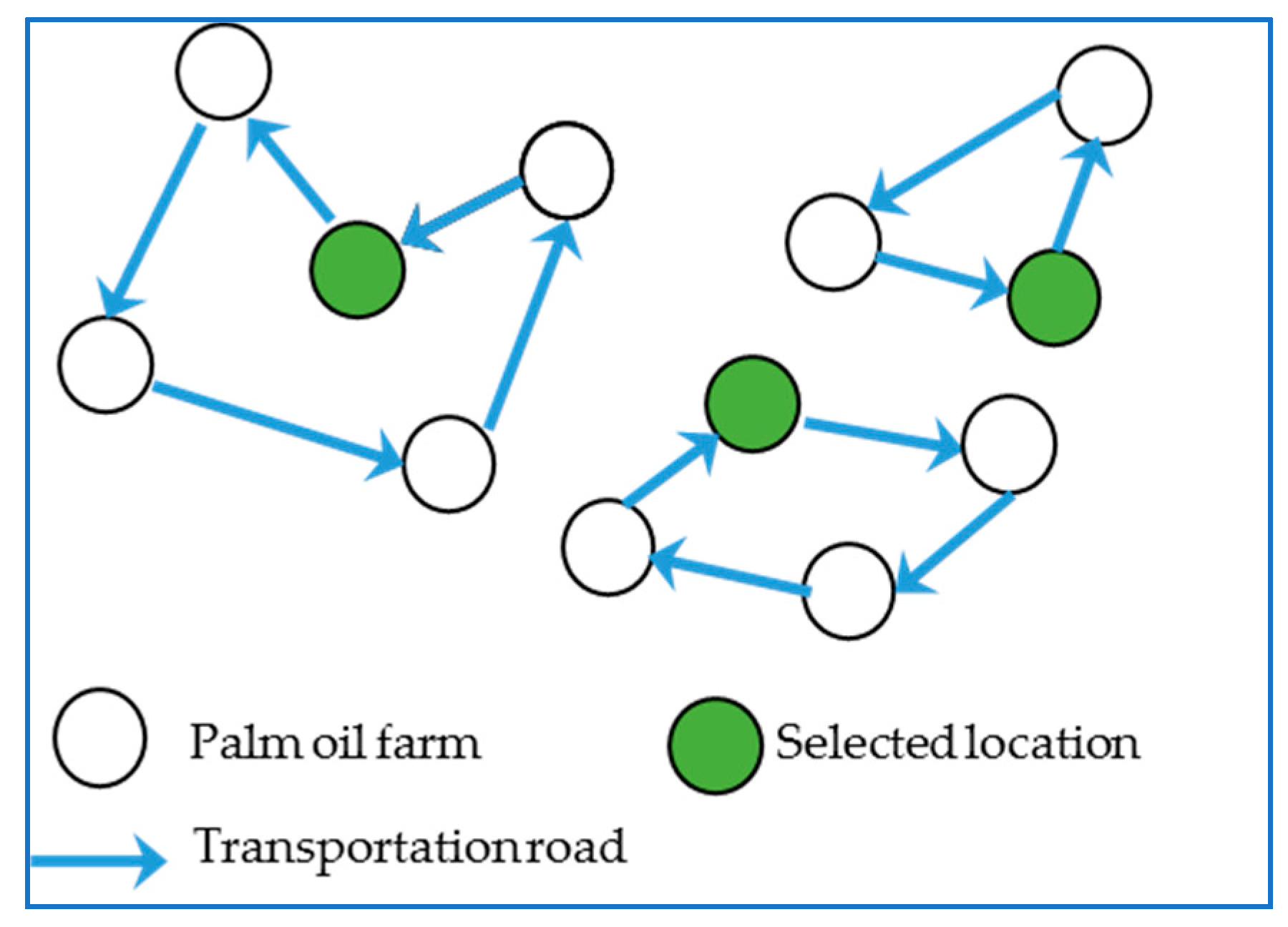
The case study consisted of 80 palm oil farms. These farms can be selected as the collection center. We aimed to choose the suitable location and set transportation route as shown in Figure 1.

The objective was to minimize the total cost. According to fuel consumption cost, we categorized the roads into five types, which were classified by using the average driving speed and the fuel consumption rate that was adopted from Akararungruangkul and Kaewman [32].

Table 1. The road type and fuel consumption rate.

Road Type	Average Speed (km/hr)	Fuel Consumption Rate (Liter/km)
A	50	0.112
B	60	0.090
C	70	0.098
D	80	0.098
E	90	0.102

show the road type and fuel consumption rate.

Because of road condition, the average speed of vehicles is different on each road type. The wider the road is, the faster a vehicle can travel. We collected the data of speed used for the road, then calculated the average speed. After that, road type and fuel used were converted by using average speed data. The fuel consumption rate the amount (liter) of fuel used after travelling 1 kilometer. A road type metric of 6 palm oil farms was used, as shown in

Table 2. Road type from farm to farm.

	1	2	3	4	5	6
1	-	A	C	B	B	C
2	A	-	B	C	A	A
3	C	B	-	B	B	C
4	B	C	B	-	D	A
5	B	A	B	D	-	C
6	C	A	C	A	C	-

.

From the distance metric shown in

Table 3. Distance from farm to farm.

	1	2	3	4	5	6
1	-	12	34	32	22	18
2	12	-	23	26	14	19
3	34	23	-	37	11	21
4	32	26	37	-	24	13
5	22	14	11	24	-	34
6	18	19	21	13	34	-

, the fuel consumption rate was multiplied by the distance of farm location. Finally, we obtained the fuel consumption metric of the road for travelling between six farms as shown in

Table 4. The fuel consumption metric.

	1	2	3	4	5	6
1	-	1.344	3.332	2.880	1.980	1.764
2	1.344	-	2.070	2.548	1.568	2.128
3	3.332	2.070	-	3.330	0.990	2.058
4	2.880	2.548	3.330	-	2.352	1.456
5	1.980	1.568	0.990	2.352	-	3.332
6	1.764	2.128	2.058	1.456	3.332	-

. For example, the distance from farm 1 to farm 2 is 12 kilometer; the type of road is A and the fuel consumption rate is 0.112 liter/km. Thus, the fuel consumption was 12 (0.112) = 1.344 liter.

For the traditional LRP, the travelling cost would directly depend on the distance, but this is not the case for the current LRP model. The distance from farm 2 to farm 3 and the distance from farm 2 to farm 6 are 23 km and 19 km, respectively. On the other hand, the fuel consumptions from 2–3 and 2–6 are 2.070 liter and 2.128 liter, respectively, which shows that in some routes, the fuel consumption is not increased because of the distance, but rather caused by road conditions.

Another example: we consider a different routing in case farm 1 was selected to be the collection center. Therefore, the two possible routings were 1-4-2-6-5-3-1 and 1-4-3-2-5-6-1, which have a total distance of 156 km and 158 km and fuel consumptions of 15.210 liter and 14.944 liter, respectively. However, the traditional LRP model selects routing of 1-4-2-6-5-3-1 because it concerns with the distance minimization. On the contrary, fuel consumption model chooses routing 1-4-3-2-5-6-1, which found that the shorter path consumes more fuel than the longer path. Nevertheless, this study focused on fuel consumption.

Vehicle condition is also a factor of fuel consumption rate. For example, heavy duty trucks usually consume more fuel than small trucks. Moreover, the age of the trucks also affects fuel consumption. The older the trucks, the more fuel is needed due to the decrease of capability of engine. This paper assumed an attribution of the vehicle, then classified them into three types categorized by age and different fuel rate consumption as shown in

Table 5. The vehicle type and fuel consumption rate.

Vehicle Type	Fuel Consumption Rate (Liter/km)
X	0.226
Y	0.247
Z	0.281

.

3.2. Mathematical Model

This section present the formulation of mathematical model used to compute the LRP problem of the case study.

Indices

V        Set of node

i         Potential collecting centers

j         Palm oil farms

k        Vehicle

 

Parameters

n           Total of the farms

FR_ijk     Fuel consumption rate from node i to node j by vehicle k

dis_ij       Distance from node i to node j

f_c           Fuel cost

E_i          Fixed cost in opening node i to be collecting center

H_i         Fixed cost of vehicle using by collecting center i

Q_k        Capacity of vehicle k

d_j          Palm oil quantity of farm j

P_i         Capacity of collecting center i

 

Decision Variables

X_ijk = 1 if travel from the node i to the node j by the vehicle k; i, j ∈ {N\{0} | i ≠ j and k = 1, 2…, q}

       = 0 otherwise

Y_i = 1 if collecting center i is opened

     = 0 otherwise

Z_ij = 1 if farm j is assigned to collecting center i

      = 0 otherwise

Objective function

$$\mathrm{Minimize}\mathrm{Total}\mathrm{cost}={\displaystyle \sum _{i\in I}}{E}_i{Y}_i+{\displaystyle \sum _{i\in V}}{\displaystyle \sum _{j\in V}}{\displaystyle \sum _{k\in K}}F{R}_{ijk}di{s}_{ij}{f}_c{X}_{ijk}+{\displaystyle \sum _{k\in K}}{\displaystyle \sum _{i\in I}}{\displaystyle \sum _{j\in J}}{H}_i{X}_{ijk}$$

(1)

Constraints

$${\displaystyle \sum _{k\in K}}{\displaystyle \sum _{i\in V}}{X}_{ijk}=1,\forall j\in J$$

(2)

$${\displaystyle \sum _{j\in J}}{d}_i{\displaystyle \sum _{i\in V}}{X}_{ijk}=Qk,\forall k\in K$$

(3)

$${\displaystyle \sum _{j\in J}}{d}_i{Z}_{ij}\le PiYi,\forall i\in I$$

(4)

$${\displaystyle \sum _{j\in V}}{X}_{ijk}-{\displaystyle \sum _{j\in V}}{X}_{jik}=0,\forall i\in V,k\in K$$

(5)

$${\displaystyle \sum _{i\in I}}{\displaystyle \sum _{j\in J}}{X}_{ijk}\le 1,\forall k\in K$$

(6)

$${\displaystyle \sum _{i\in S}}{\displaystyle \sum _{j\in S}}{X}_{ijk}\le \left|S\right|-1,\forall S\subseteq J,k\in K$$

(7)

$${\displaystyle \sum _{j\in J}}{X}_{ijk}+{\displaystyle \sum _{i\in V\backslash \left\{j\right\}}}{X}_{jik}\le 1+Z_{ij},\forall i\in I,j\in J,k\in K$$

(8)

X_ijk = 0,1 ∀i∈I, j∈V, k∈K

(9)

Y_i = 0,1 ∀i∈I

(10)

Z_ij = 0,1 ∀i∈I, j∈V

(11)

The objective function (1) measures the total cost consist of the fixed cost of opening the collection center and the fuel consumption cost using for transportation and the fixed cost related with vehicle uses. Constraint (2) ensures that each customer is in exactly one route and each has only one predecessor in the route. Constraints (3) and (4) are capacity constraints related to the vehicles and collection center. Constraints (5) and (6) assure the continuity of each route and terminate at the depot where the route starts. Constraint (7) is a sub-tour elimination constraints which said that for any subset S of the set of customers J and for any route k, the number of arcs belonging to route k that connect the members of S, must not exceed the cardinality of S-1. Constraint (8) ensures that a customer must be assigned to a depot if there is a route connecting them. Finally, constraints (9), (10) and (11) specify the binary variables used in the formulation.

4. Solution Approach

We propose a heuristic method based on Adaptive Large Neighborhood Search (ALNS) as the solution to this problem. The ALNS framework was presented by Rope and Pisinger [22] to solve the variant of combinatorial optimization problem such as VRP and LRP. They developed the Large Neighborhood Search (LNS), which was introduced by Shaw [33] for the Capacitated Vehicle Routing Problem (CVRP). The procedure starts with an initial solution and gradually improves objective value. A destroy and repair operator are applied in each iteration. The destroy operator removes a small group of customers randomly, while the repair operator reinserts them to improve objective value. Furthermore, Ropke and Pisinger [22] proposed an ALNS to improve LNS, which allowed the ALNS to use several destroys and repair methods in the same search iteration. In each iteration, the operator would destroy part of the current solution and repair it in a different way to create a new solution. Destroy and repair operators are selected according to an adaptive probability mechanism, and in each iteration, the operator has a probability of which the weights are adjusted dynamically depending on how well it has performed in the past.

In this paper, however, we have adapted the ALNS algorithm of Lutz [34], in which the ALNS starts with initialization of solution then select destroy and repair operator applying to the solution. Let D = {d_i | i = 1,…, k} be the set of destroy operator and R = {r_i | i = 1,…, l} be the set of repair operator. The initially equal weights of the operators are denoted by w(r_i) and w(d_i). During the runtime, these weights are adjusted periodically and an updated period contains p_u iterations. The selection of these operators of each iteration is based on their weights. The structure of ALNS is shown in Algorithm 1.

Algorithm 1. Adaptive Large Neighborhood Search (ALNS) algorithm.

Input problem instant I create initial solution smin = s ∈ S(I) while stopping criteria not met do         for i = l,…, pu do               select r ∈ R, d ∈ D according to probability p               s’ = ri (di(s))               if accept (s, s’) then                     s = s’                     if c(s) < c(smin) then                             smin = s         adjust the weight w and probability p of the operators return smin

4.1. Initial Solution

We constructed the initial solution with the following steps:

Step 1:

Sorting the candidate locations as the product quantity by descending order, then calculate the accumulation probability of each based on their product quantity. Next, randomly select the location of the collection center by using a roulette wheel. The location thus has more product quantity as well as more chance to select.

Step 2:

Assigning a farm to collection center follow fuel consumption; the farm that has the lowest fuel cost can be selected first.

Step 3:

Assigning to the next farm through sequence of fuel consumption. Meanwhile, the total amount of products needs to be checked to match with vehicle and collection center constraints. When the capacity has satisfied the constraint, the assignment can be stopped.

Step 4:

If there are farms left over, return to step 1-3 to open the next collection center and assign tasks for the farms.

Step 5:

If there are no other farms, the procedure is terminated.

4.2. Degree of Destruction

Degree of destruction (d) is the level of eradication that is applicable to the current solution. For example, the current solution contains 30 farms and the degree of destruction is equivalent to 20%, which means we need to remove six farms (30 × 0.2) from the current solution. Then, set q = 6 and put them into the customer pool, and the repair operator puts them back and creates a new solution. We designed the selection degree of destruction randomly from the interval {10%, 15%, 20%, 25%, and 30%} in every iteration.

4.3. Destroy Operators

The following describe the destroy operators used in the algorithm.

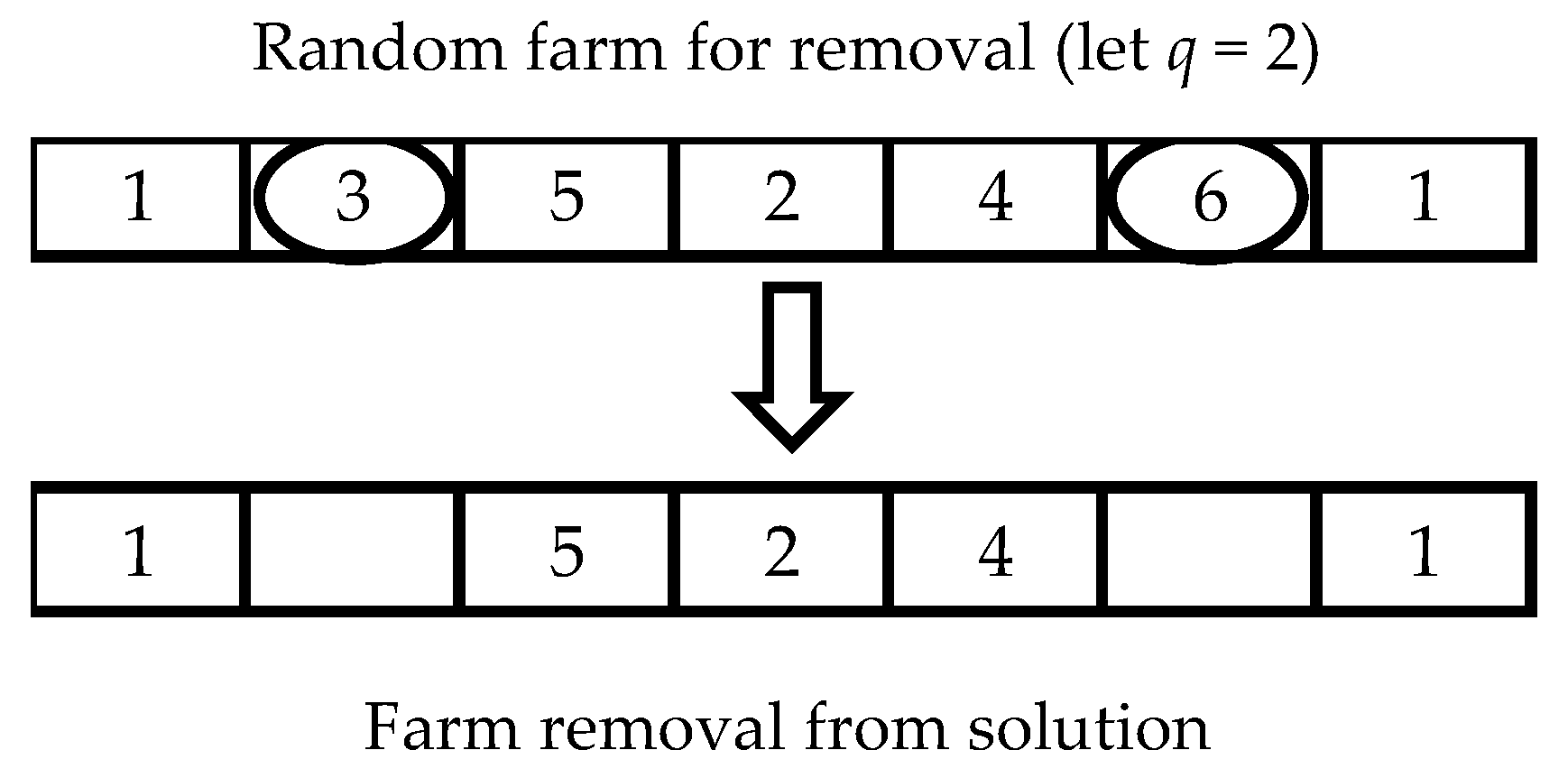
4.3.1. Random Removal (RaR)

This operator is a simple method in which q farms are chosen randomly and removed from the solution, as shown in Figure 2.

Step 1:

Randomly choose q farms from the current solution.

Step 2:

Remove them from the current solution to the customer pool.

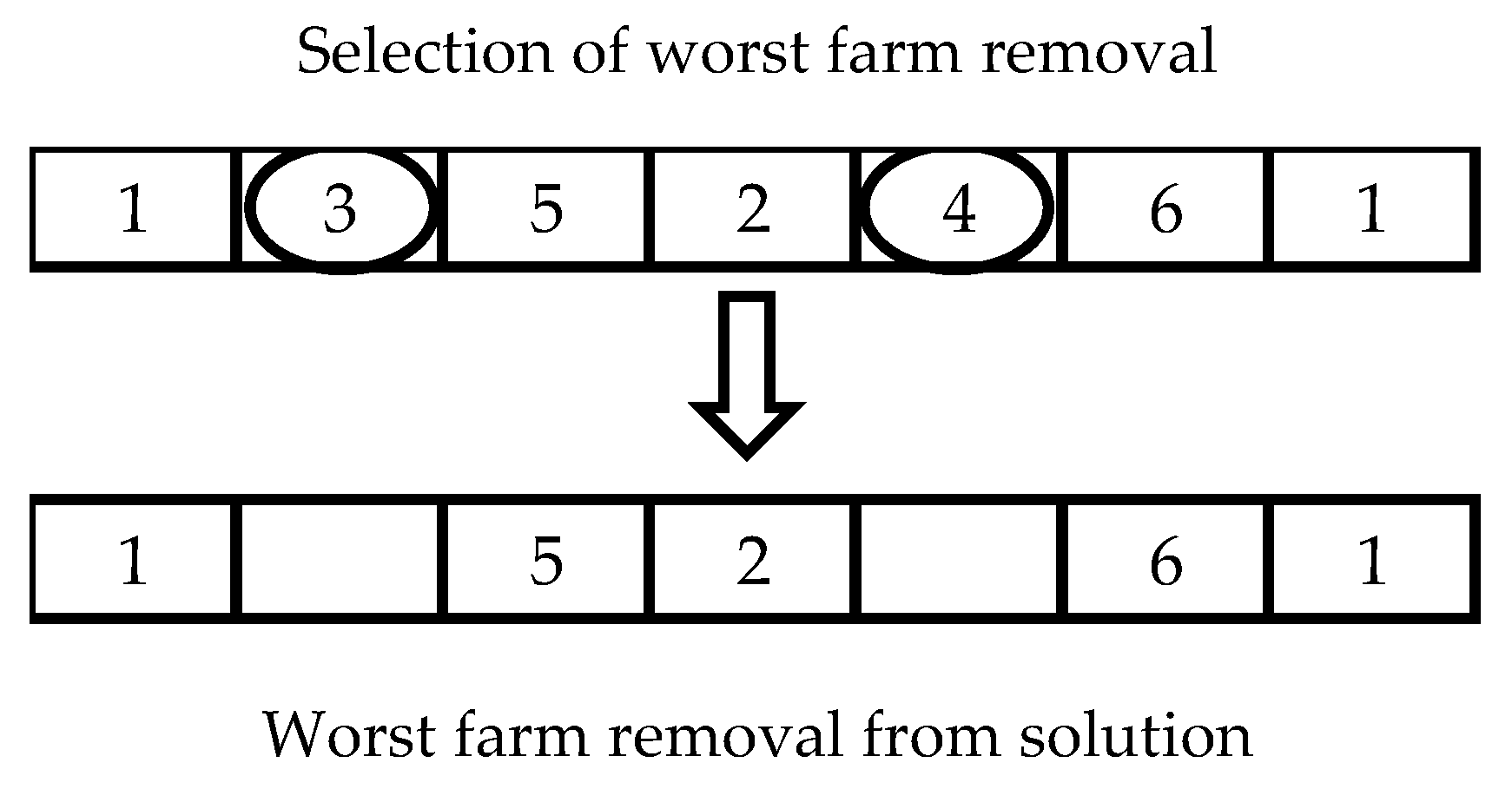
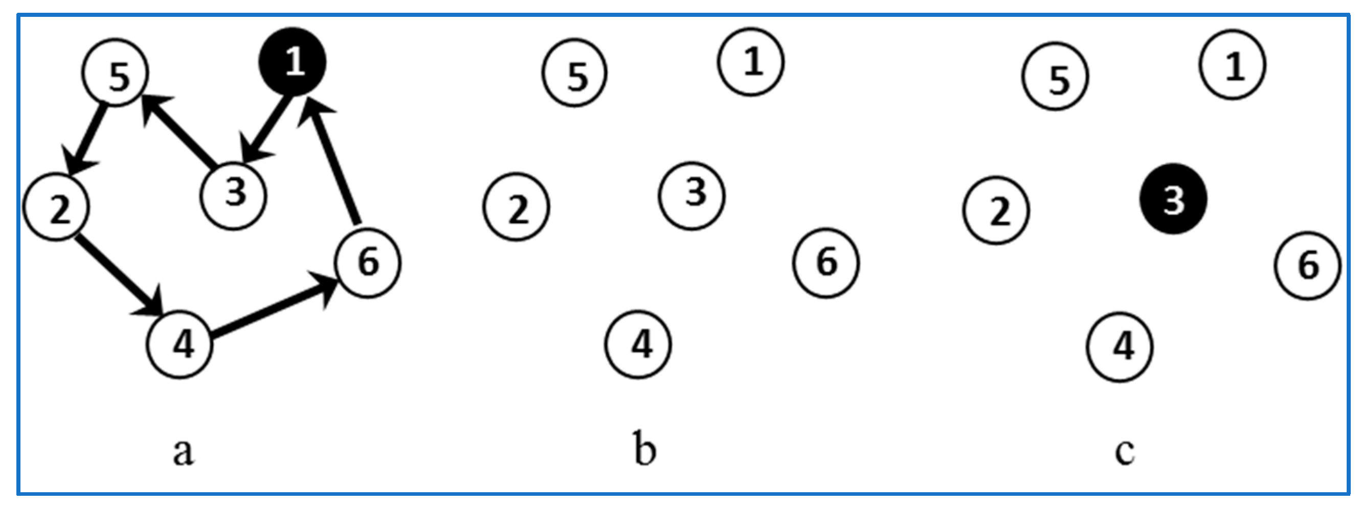
4.3.2. Worst Removal (WoR)

The worst removal entails removing the worst value in order to improve the solution. This operator considers the highest cost in current solution, shown in Figure 3.

Let the current solution be {1-3-5-2-4-6-1} and q = 2. This means farm location number 1 is selected to be the collection center.

Step 1:

Calculate the total fuel consumption of this routing by using data in Table 4, 11.658 liter (3.332 + 0.990 + 1.568 + 2.548 + 1.456 + 1.764).

Step 2:

Remove farms one by one, then calculate the remaining total fuel consumption. According to the example of removal farm number 3 from the current solution, the routing is changed to {1-5-2-4-6-1}. The remaining total fuel consumption is 9.316 liter (1.980 + 1.568 + 2.548 + 1.456 + 1.764). When we remove farm numbers 3,5,2,4 and6 from the current solution, the remaining total fuel consumptions are 9.316, 11.170, 9.894, 9.782, and 11.318, respectively.

Step 3:

Calculate the different values between the current solution (step 1) and the solution without each farm (step 2). The different maximum value will be removed. The different value without farm numbers 3,5,2,4,6 are 2.342(11.658 − 9.316), 0.488, 1.764, 1.876 and 0.340, respectively.

Step 4:

Ranking the farms by considering the different value by decreasing order. Thus, the list of farms who have to be removed are number 3,4,2,5 and 6 respectively and set to q = 2; thus farms number 3 and 4 will be removed.

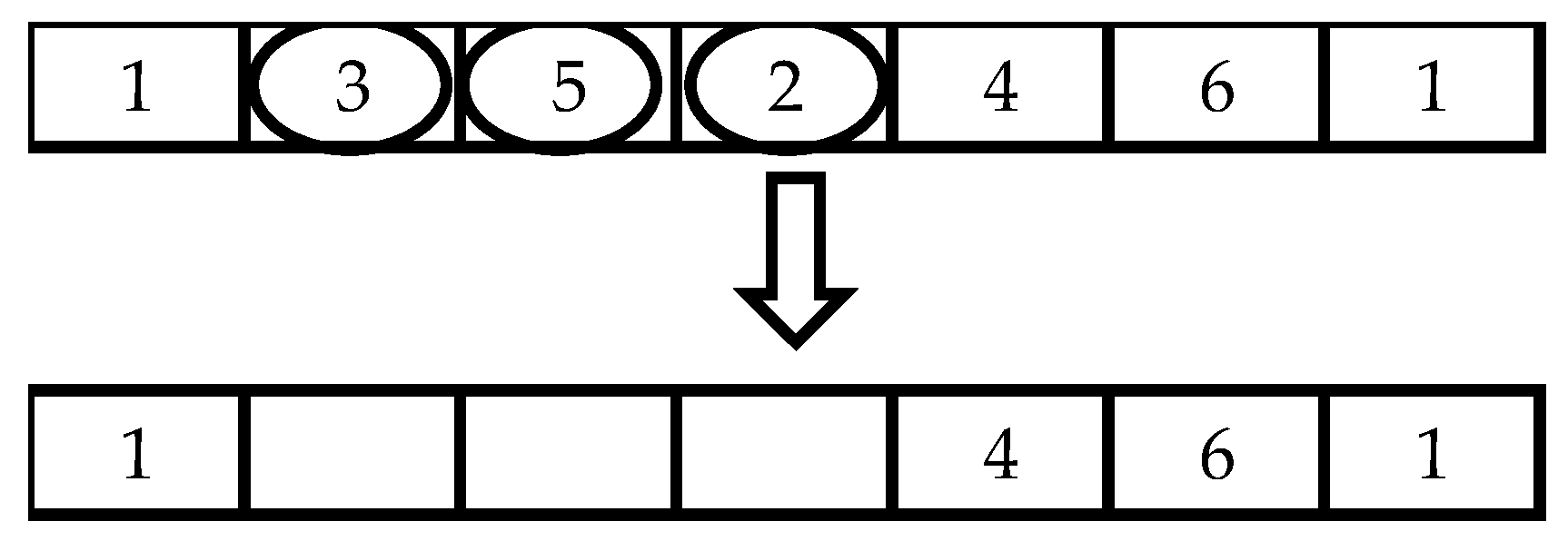
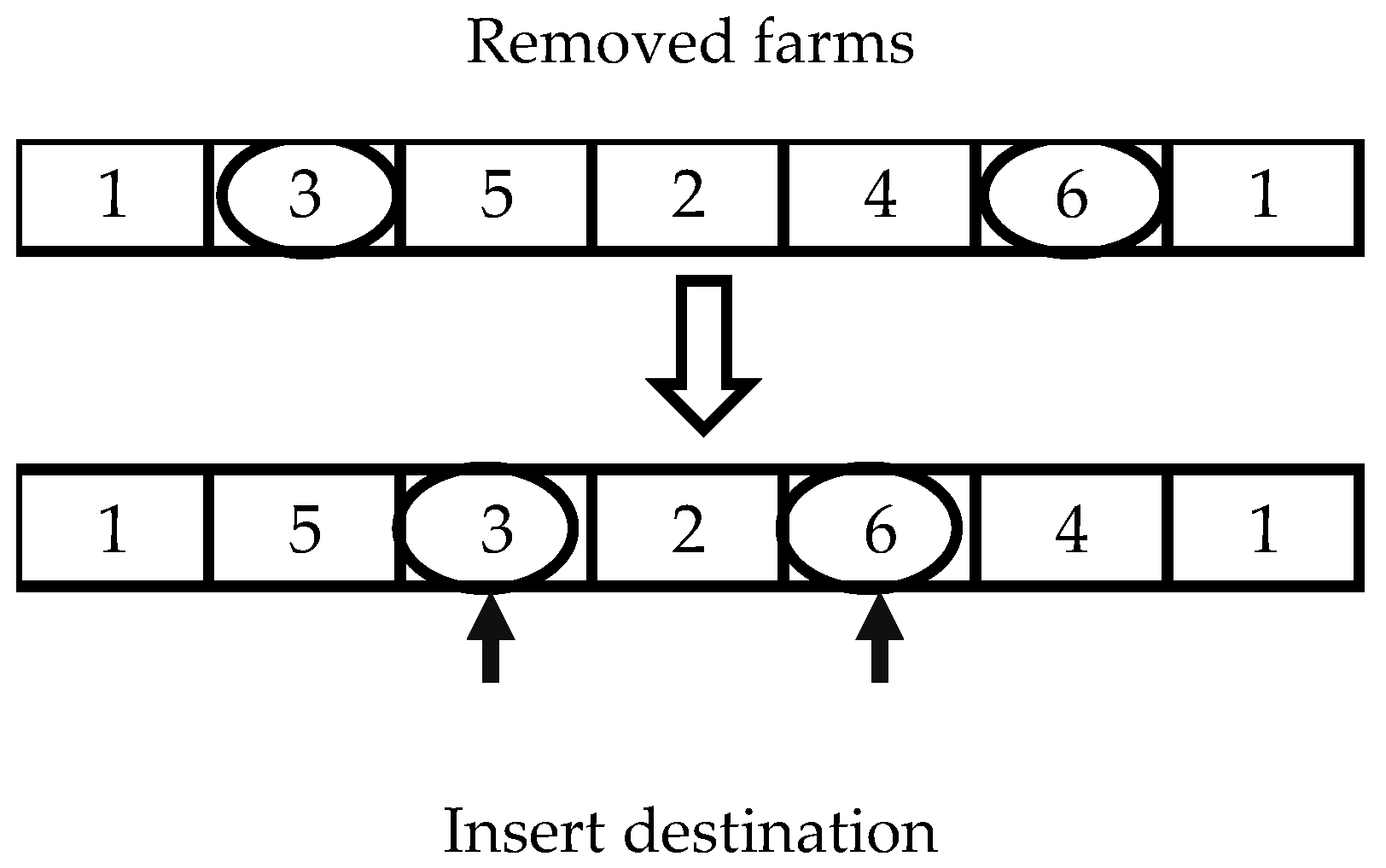
4.3.3. Related Removal (ReR)

This operator is similar to the one used by Hemmelmayr et al. [35]. A farm is randomly selected for removal from the solutions as shown in Figure 4.

Let the current solution be {1-3-5-2-4-6-1} and q = 3.

Step 1:

Randomly choose a farm (a seed farm), for instance number 2.

Step 2:

Select q − 1 farms that consume the least amount of fuel when traveling to the seed farm. For example, the fuel consumptions when traveling from farm number 2 to numbers 3,4,5 and 6 are 2.070, 2.548, 1.568 and 2.128, respectively (see Table 4). Select two farms (q − 1): numbers 5 and 3.

Step 3:

Remove those farms from the current solution to the customer pool.

4.3.4. Collecting Centre Removal (CcR)

Step 1:

Among all the opened collection centers, randomly choose one and close it.

Step 2:

All assigned farms are removed and put into the customer pool.

Step 3:

Randomly choose another one which is not opened yet and open it.

This operator is also important for diversification. Figure 5 illustrate the method of this operator.

4.4. Repair Operators

The repair operators re-insert the customers from the pool to the solution.

4.4.1. Random Insertion (RaI)

The farms which are removed from the destroy method are inserted randomly in both position and order as shown in Figure 6.

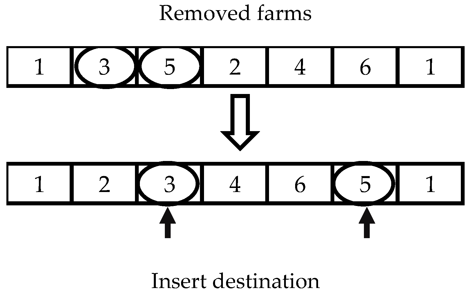
4.4.2. Best Insertion: (BeI)

This operator is a solution improvement to find the best position of insertion considering minimal fuel consumption as shown in Figure 7.

Let the current solution be {1-3-5-2-4-6-1} and q = 2 as well as considering the removed farms number 3 and 5.

Step 1:

Attempt to insert farms in the routing that generate the lowest fuel consumption.

Step 2:

Repeat step 1 until all the removed farms are inserted.

In the example of having farm 3 and 5 removed by the destroy method, the current solution is {1-2-4-6-1}, after which step 1 is performed, which requires farm number 3 to be inserted in all of the positions. The possible insertions are therefore 1-3-2-4-6-1, 1-2-3-4-6-1, 1-2-4-3-6-1 and 1-2-4-6-3-1; fuel consumptions are 11.172, 9.964, 11.044 and 10.738, respectively. Thus, inserting farm number 3 of position 1-2-3-4-6-1 is the lowest fuel consumption. In this way, we can insert farm number 5.

4.5. Adaptive Weight Adjustment and Acceptance Criteria

Let w(h) is the weight of an operator h which is either a destroy or repair operator and p_u is the update duration, i.e., the non-improved number of iteration. The amount of period time the operator h has been used throughout the p_u iterations is called u_h. The success s(h) of h is set to zero at the start of p_u iterations. After h is used in an iteration, s(h) is improved by ω_i if the new solution is of corresponding quality:

ω₁ = 10

If the new solution is the new global best.

ω₂ = 7

If the new solution is better than the current.

ω₃ = 4

If the new solution does not improve the current, it is accepted as the next current solution.

ω₄ = 1

If the new solution does not improve the current and it is not accepted as the next current solution.

The purpose of making the decision of the acceptance criteria of ALNS is whether to proceed with the previous solution (s) or with the new solution (s’); the purpose of all acceptance criteria is to accept solutions that improve the current situation. However, there are some criteria that allow them to accept non-improving solutions. There are different ways in previous studies which have attempted to solve this problem. Shaw [32] proposed the Greedy acceptance method. This method does not accept any worse solutions than the previous one. This might be the limitation of the search because the worse solutions are not fully considered, but often rejected at first sight. Ropke and Pisinger [22] used a simulated annealing (SA) as an acceptance criteria. This is one of the most popular acceptance method for the ALNS algorithm. Thus, we used the SA acceptance criterion in this paper, in which all improving solutions s’ are accepted or rejected with probability $p=\exp (c\left(s\right)-c\left(s^{\prime }\right)/kT$, where T is the temperature of the considered iteration and k is the constant used in the probability function to determine whether to accept a worse solution or not.

5. Computational Result

We performed the testing of mathematical model by Lingo program V.11 and the ALNS algorithm (CPU: Intel Core i5 up to 2.7 GHz, RAM: 4 GB). The three datasets were provided and tested which the datasets of sample consisted of small (n = 10), medium (n = 30) and large (n = 50). The parameters of the test instances were randomly generated using uniform distribution. The distances between the farm locations were randomly generated from 10 km to 50 km. The capacity of the collection center and the vehicles included three levels; 10,000 kg, 20,000 kg and 30,000 kg. The palm oil quantities were randomly generated from 500 kg to 6000 kg. The simulation was run for five times and the best solution was selected to be the representative of the algorithm. The stopping criterion was the number of iteration which was set to 500 iterations. Finally, we used the algorithm to solve the case study problem. The result from the Lingo program and the ALNS algorithm are shown in

Table 6. The result comparison of exact method and ALNS algorithm.

Dataset	No.	Farm	Lingo Program			ALNS		Difference
			Status	Total Cost (Baht)	Processing Time (h)	Total Cost (Baht)	Processing Time (h)	Total Cost (Baht)	Processing Time (h)	% Gap Total Cost	% Gap Processing Time
Small	Sm. 1	10	Global Opt	1,021,377	00:01:24	1,021,377	00:01:24	0	00:00:00	0	0.00%
	Sm. 2	10	Global Opt	1,032,533	00:01:36	1,032,533	00:01:35	0	00:00:01	0	1.04%
	Sm. 3	10	Global Opt	1,033,765	00:01:32	1,033,765	00:01:31	0	00:00:01	0	1.09%
	Sm. 4	10	Global Opt	1,049,518	00:01:28	1,049,518	00:01:28	0	00:00:00	0	0.00%
	Sm. 5	10	Global Opt	1,051,763	00:01:34	1,051,763	00:01:33	0	00:00:01	0	1.06%
Average				1,037,791	00:01:31	1,037,791	00:01:30	0	00:00:01	0	0.64%
Medium	Me. 1	30	Feasible	2,065,619	16:09:17	2,065,720	00:05:36	−101	16:03:41	−0.005%	99.77%
	Me. 2	30	Feasible	2,068,392	21:24:15	2,068,678	00:06:27	−286	21:17:48	−0.014%	99.76%
	Me. 3	30	Feasible	2,068,690	22:38:28	2,068,706	00:06:32	−16	22:31:56	−0.001%	99.78%
	Me. 4	30	Feasible	2,073,662	19:34:42	2,073,762	00:05:54	−100	19:28:48	−0.005%	99.77%
	Me. 5	30	Feasible	2,074,331	21:00:15	2,074,413	00:05:15	−82	20:55:00	−0.004%	99.78%
Average				2,070,139	20:09:23	2,070,256	00:05:57	−117	20:03:27	−0.006%	99.77%
Large	La.1	50	Lower bound	4,055,126	>120	4,055,137	00:13:56	−11	119:46:04	0.000%	99.81%
	La.2	50	Lower bound	4,056,264	>120	4,056,280	00:16:27	−16	119:43:33	0.000%	99.77%
	La.3	50	Lower bound	4,056,541	>120	4,056,639	00:14:52	−98	119:45:08	−0.002%	99.79%
	La.4	50	Lower bound	4,053,720	>120	4,053,880	00:15:54	−160	119:44:06	−0.004%	99.78%
	La.5	50	Lower bound	4,058,125	>120	4,058,205	00:12:45	−80	119:47:15	−0.002%	99.82%
Average				4,055,955	120	4,056,028	00:14:47	−73	119:45:13	−0.002%	99.79%

.

5.1. Three Datasets of Sample

According to Table 6, the five small problems shown a global optimal status on Lingo that was only 1 second different in Sm.2, Sm.3 and Sm.5 which could be concluded the Lingo program and the ALNS algorithm calculated the same results for this sample size. As a result, the small-sized sample contain 10 farms, so the problem was not complicated. The optimal solution for all small problems was the average total cost at 1,037,791 Baht. Moreover, there was no gap between Lingo program and ALNS algorithm, thus, the ALNS algorithm was effectively equal to the Lingo program for small-sized samples.

For medium-sized samples, the result from ALNS was a different total cost compared with the Lingo program. Although the ALNS result was slightly higher than the Lingo result, the Lingo program required a longer processing time than ALNS. The Lingo program took an average processing time of 20.03 h but ALNS took only 5.57 min; in other words, it was able to reduce the processing time by 99.77%. Therefore, the Lingo program consumed long processing time as the number of farms increase.

For the large-sized sample, the Lingo program could not find a global or feasible solution even though it had been taking more than 120 h of processing time. The Lingo program was able to find a lower bound, which was compared with the ALNS result. The total cost obtained by ALNS was slightly higher than Lingo result. However, the ALNS algorithm provided the acceptable result with a fast processing time. The ALNS algorithm had taken only 14.47 min of processing time which was able to reduce the computational time by 99.79%. Therefore, the Lingo program seemed ill-fitted for large samples.

We performed the analysis using statistical methods to compare the performance. The result of total cost and processing time of all problem sizes were tested normality with a 95% level of confidence as shown in

Table 7. Normality testing of Lingo and ALNS.

	Small		Medium		Large
Total Cost	Exact	ALNS	Exact	ALNS	Exact	ALNS
p-value	0.418	0.418	0.330	0.291	0.854	0.886
Result	Normal	Normal	Normal	Normal	Normal	Normal
Processing Time	Exact	ALNS	Exact	ALNS	Exact	ALNS
p-value	0.740	0.831	0.651	0.578	0.378	0.847
Result	Normal	Normal	Normal	Normal	Normal	Normal

which all the p-values were greater than 0.05. Therefore, the data for all datasets were normal distribution and after that the data of all datasets were tested for the average difference using a paired t-test with a 95% level of confidence and the results were presented in

Table 8. Result of paired t-test from all datasets.

Dataset	p-value
	Total Cost	Processing Time
Small	1.000	0.070
Medium	0.060	0.000 *
Large	0.058	0.000 *

* Significant difference of method.

.

From Table 8, the statistics showed a significant p-value greater than 0.05 of total cost for all datasets. It was insignificant difference between the Lingo program and ALNS algorithm with a 95% level of confidence. The processing time for the small-sizes sample had p-value greater than 0.05, denoted that insignificant difference between two method. However, the processing time for the medium-sized sample and the large-sized sample had a p-value of less than 0.05, which denoted a significant difference between the Lingo program and ALNS algorithm. Therefore, the ALNS algorithm was able to reduce the processing time while finding a total cost was not different compared to the Lingo’s result. The ALNS algorithm was the optimal method for solving the location routing problem with a large number of farms.

5.2. The Case Study

We applied the ALNS algorithm for solving the case study problem, which was conducted to demonstrate how the propose model could be used for the palm oil collection location routing problem. The opened location, routing plan and total cost in each collection center are summarized in

Table 9. Case study result.

Opened Location	Optimal Routes	Total Palm oil (kg)	Total Cost (Baht)
14	14-6-9-8-22-12-14	19,270	621,415
18	18-26-27-28-18	19,846	621,588
25	25-5-15-1-4-19-25	19,983	621,723
3	3-2-7-17-16-11-3	18,578	621,498
13	13-23-20-29-30-21-10-24-13	18,929	621,805
76	76-42-55-32-38-45-76	19,275	621,875
61	61-33-40-54-48-65-71-61	18,953	621,982
46	46-31-52-60-72-34-46	19,096	621,663
68	68-35-44-66-49-68	18,921	621,532
36	36-41-73-79-56-39-36	18,909	621,774
51	51-37-43-47-50-59-51	19,183	621,689
58	58-53-62-67-77-70-58	19,660	621,852
64	64-63-57-69-75-74-78-80-64	19,230	621,668
Total			8,082,064

.

There were 80 customers (farm groups) in the case study. The exact method could not find the solution in spite of taking processing time over 120 hours. On the other hand, ALNS took an average of 20.46 min and came along with the solution as showed in

Table 10. Comparison of the proposed ALNS and Lingo on case study problem (n = 80).

Run	Lingo Program		ALNS
	Total Cost (Baht)	Processing Time (h)	Total Cost (Baht)	Processing Time (h)
1	N/A	>120	8,343,126	00:21:07
2	N/A	>120	8,342,341	00:23:18
3	N/A	>120	8,344,554	00:19:25
4	N/A	>120	8,344,128	00:19:04
5	N/A	>120	8,345,297	00:20:55
Average	N/A	>120	8,343,889	00:20:46

.

As mentioned in Section 3.1, the traditional LRP dealt with distance minimization; however, our model dealt with fuel consumption minimization. The conditions of the road affected to the fuel consumption; thus, considering distance was did not minimize fuel consumption.

Table 11. Comparison of solution of fuel minimization and distance minimization in perspective of fuel cost.

Solution of Fuel Minimization		Solution of Distance Minimization
Opened location	Fuel cost (Baht)	Opened location	Fuel cost (Baht)
14	1415	14	1415
18	1588	18	1588
25	1723	26	1953
3	1498	3	1498
13	1805	15	2055
76	1875	76	1875
61	1982	61	1982
46	1663	48	1961
68	1532	63	1926
36	1774	36	1774
51	1689	51	1689
58	1852	56	2155
64	1668	67	1896
Total	22,064	Total	23,767
		Dif.	7.72%

compares the solutions of this study model to the solution from classical LRP; the distance was reduced, and it saved 7.72% of fuel cost.

To verify the effectiveness of the proposed algorithm, we compare the ALNG algorithm with the Differential Evolution (DE) algorithm from the literature [32]. This study proposed DE to solve the problem and modified some points in the original DE, called MED. The computational results are shown in

Table 12. Computational result of the DE and ALNS.

	DE-Fuel Used (L)						ALNS-Fuel Used (L)
	n	Current practice	DE	MDE-1	MDE-2	MDE-3	n	Current practice	ALNS
CASE	110	112.3	110.1	108.76	106.85	95.4	80	630.4	581.73
% difference			1.96	3.15	4.85	15.05			7.72

* % difference: percentage gap is calculated as (current practice - proposed method)/current practice.

. The ALNS has a percentage difference of fuel usage 7.72%, more than that of DE, MDE-1 and MDE-2. MDE-3 has the best performance in term of the quality of solution with 15.05% of fuel saving. However, the size of problem may effect to the percentage difference. Our problem is smaller, thus the impact of percentage difference is lower than the bigger problem.

In term of processing time, DE algorithm set stopping criteria by runtime limitation at 10 min but ALNS set that by 500 iterations. Moreover, both algorithms were tested by different computer specification. Therefore, we only present the performance of solution quality.

Figure 8 showed the nature of ALNS during searching the solution of the case study which shows that ALNS continuously improved the solution from until stopping criteria were met. During 1–70 iterations, the solution was improved rapidly. After that, the solution was gradually improved until 250 iterations, after which it was stable.

6. Conclusions and Outlook

The purpose of this study was to solve the Location Routing Problem in the case study of a palm oil collection center. The mathematical model has been formulated to minimize the total cost consisted of opening cost, fixed cost of vehicle uses and fuel cost. We have presented an ALNS algorithm for this LRP problem, which used several operators that were simple and relied on few parameters.

Three datasets were tested (small, medium and large-sized samples) and the results were compared to the exact method that was computed by the Lingo program. The objective value from Lingo and ALNS of the small-sized sample were equal. In addition, the processing time of ALNS was slightly higher than the Lingo program. For the medium and large-sized sample, ALNS calculated a higher objective value than the Lingo program but the Lingo program consumed longer processing time. Although the Lingo program had a long processing time, it found only feasible and lower bounds for medium-sized and large-sized. ALNS on the other hand, was able to find an acceptable solution within a short processing time and it was faster than Lingo program. Thus, we could summarize that ALNS was the optimal method for solving large problems.

We have also implemented ALNS of the case study problem, which was larger than the instances. The ALNS produced the solution in an average processing time of 20.46 min, while the Lingo consumed over 120 hours, but was unable to find the solution. Thus, ALNS was efficient to solve the case study problem. Furthermore, we extended a comparison between the model of fuel consumption and distance minimization with respect to fuel cost. The result showed that this model could reduce 7.72% of fuel costs as compared to the classical LRP, which is distance minimization.

The results provided by the ALNS algorithm were useful for palm oil logistic management. The suitable locations were selected to be collection center and arranged the routing plan to collect palm oil from farmers. The total costs of the system were minimized and the farmers would make more profit compared to the past. Palm oil was one of the sources of renewable energy and this research aimed to minimize fuel energy consumed as well. Therefore, this could be implied that this study considered as green logistic management work as well as environmental improvement.

Future research will focus on extending this approach to solve a larger LRP problem or another LRP variant such as 2E-LRP (2 Echelon Location Routing Problem); in the meantime, developing the ALNS is needed. Because we will solve bigger problems, the algorithm should be more efficient to compute both the high solution quality and a short processing time.

The proposed algorithm is not only used to solve the case study problem, but can also solve the similar problems. To develop the performance of the algorithm, a good software design is needed. After software development, the software can be suitable for related businesses. The license of the developed software can be customized and shared for worldwide usage. Therefore, this is not restricted to palm oil businesses, but is also an open opportunity for other fields. We can imply that the open innovation concept has been applied to the palm oil and related business. The main idea of open innovation is to look for new technologies and ideas outside of the firm for other ways to increase the efficiency and effectiveness of their innovation processes. An example of open innovation research studies can be revealed in Yun et al. [36] and Yun et al. [37].