

Prediction of Angular Distortion in Gas Metal Arc Welding of Structural Steel Plates Using Artificial Neural Networks


 ,
,  and
and 
Abstract
1. Introduction
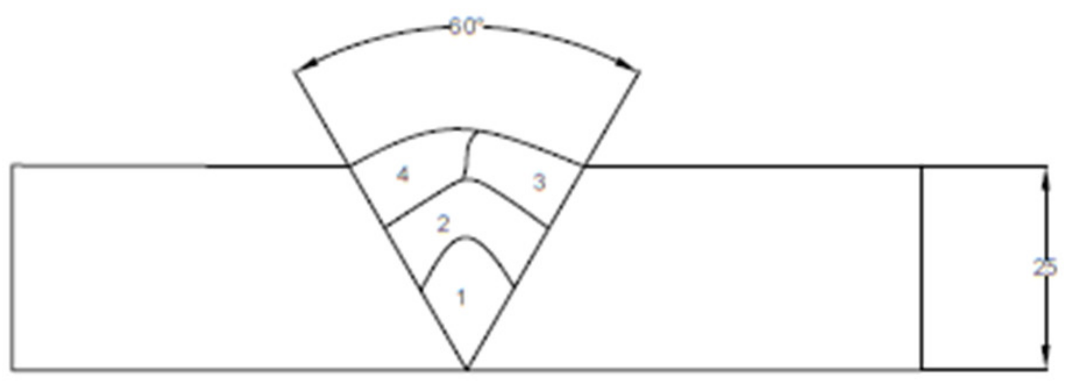
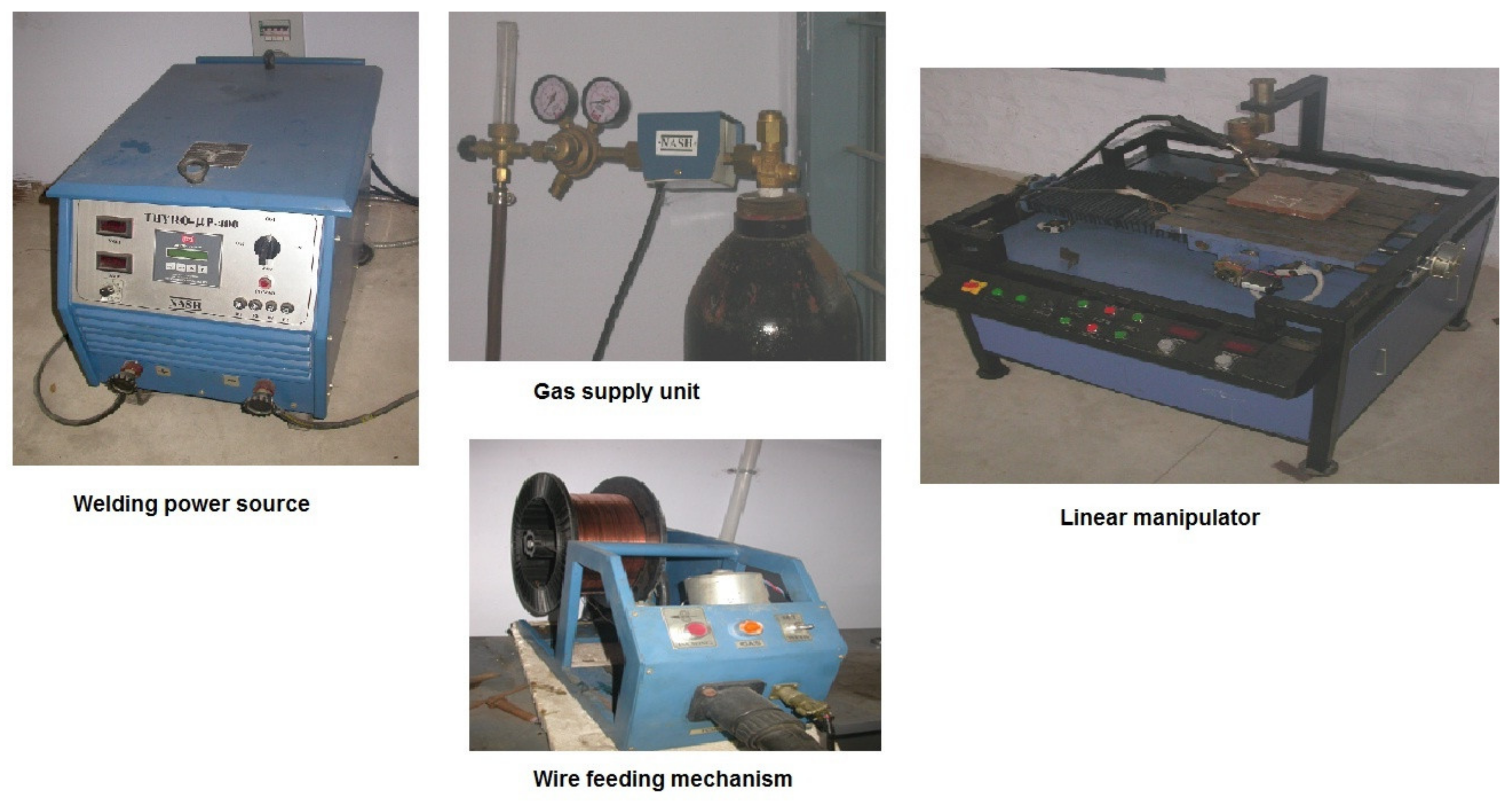
2. Experimental Process
3. Plan of Investigation
3.1. Choosing the Appropriate Design
3.2. Identification of the Process Variables
3.3. Determining the Limits of the Process Variables
- Xi—The required coded value of a variable X,
- X—Is any value of the variable from Xmin to Xmax
- Xmin—Is the lower limit of the variable.
- Xmax—Is the upper limit of the variable.
3.4. Development of Design Matrix
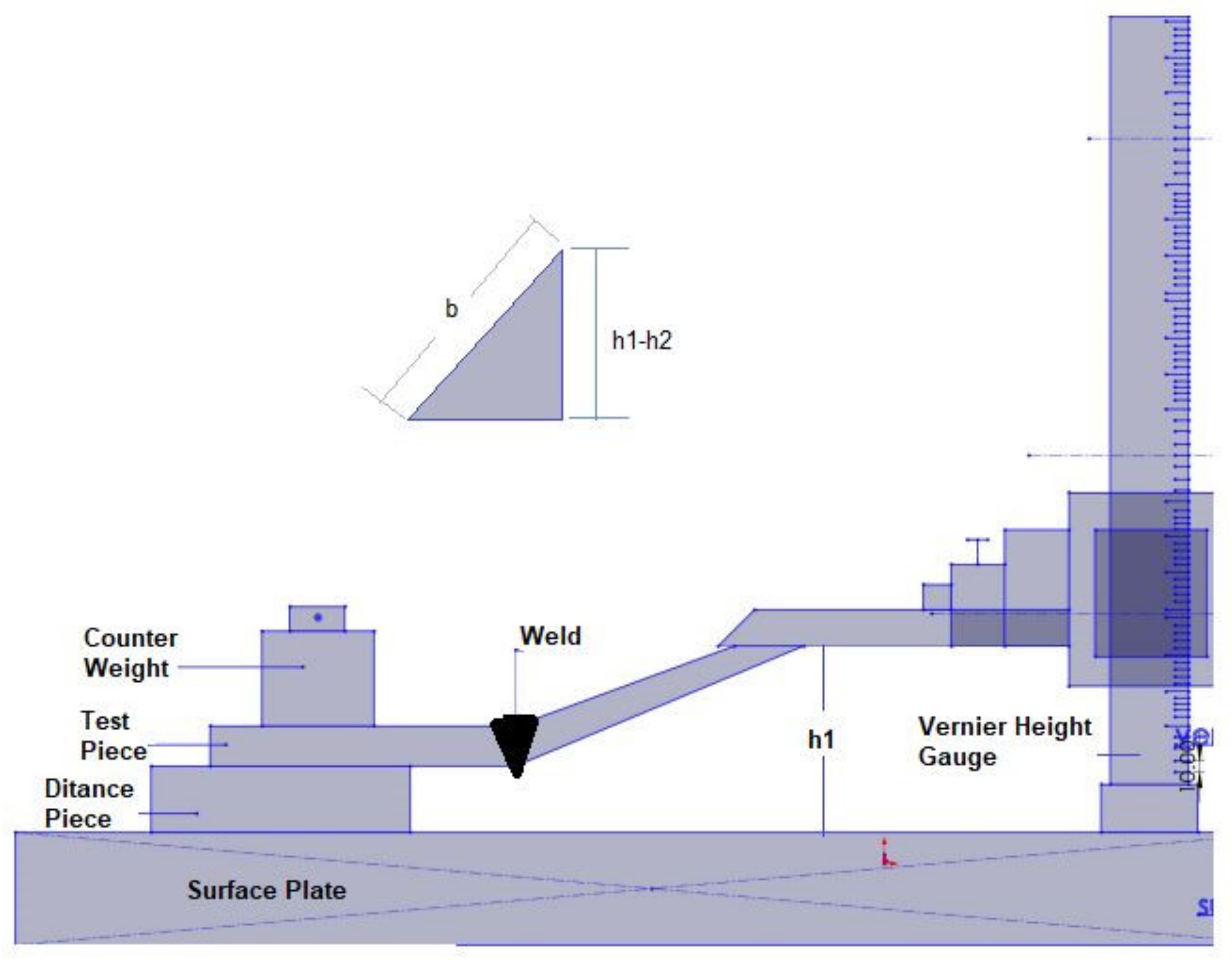
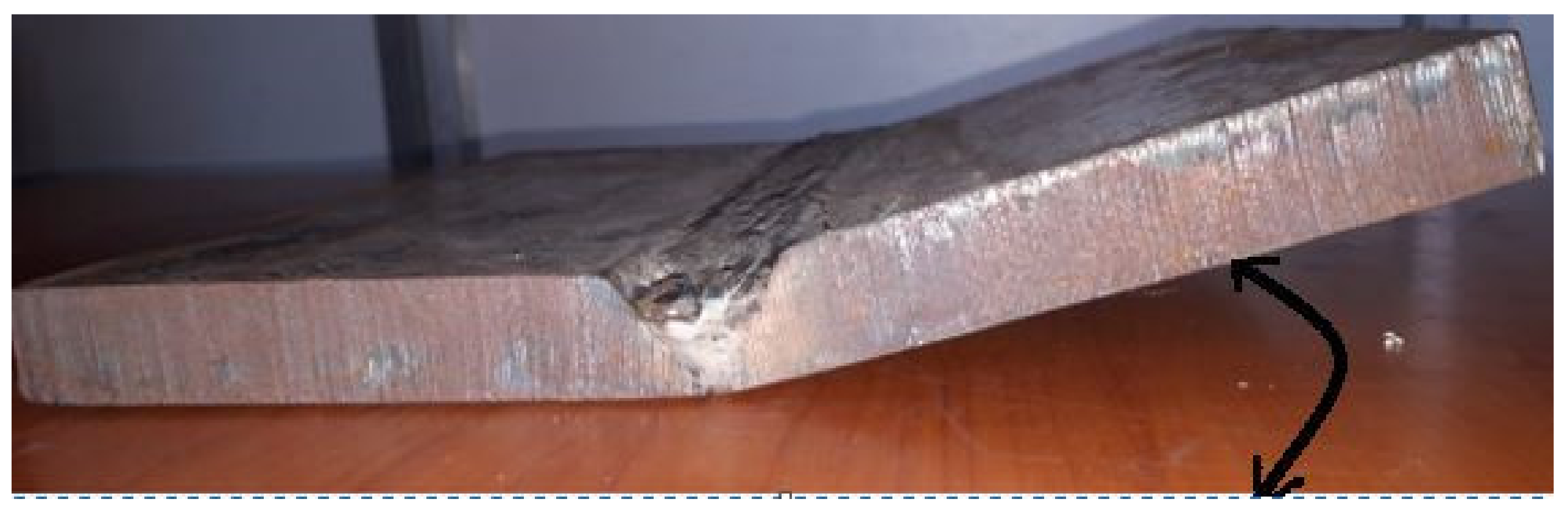
3.5. Measurement of Angular Distortion
4. Mathematical Model Development
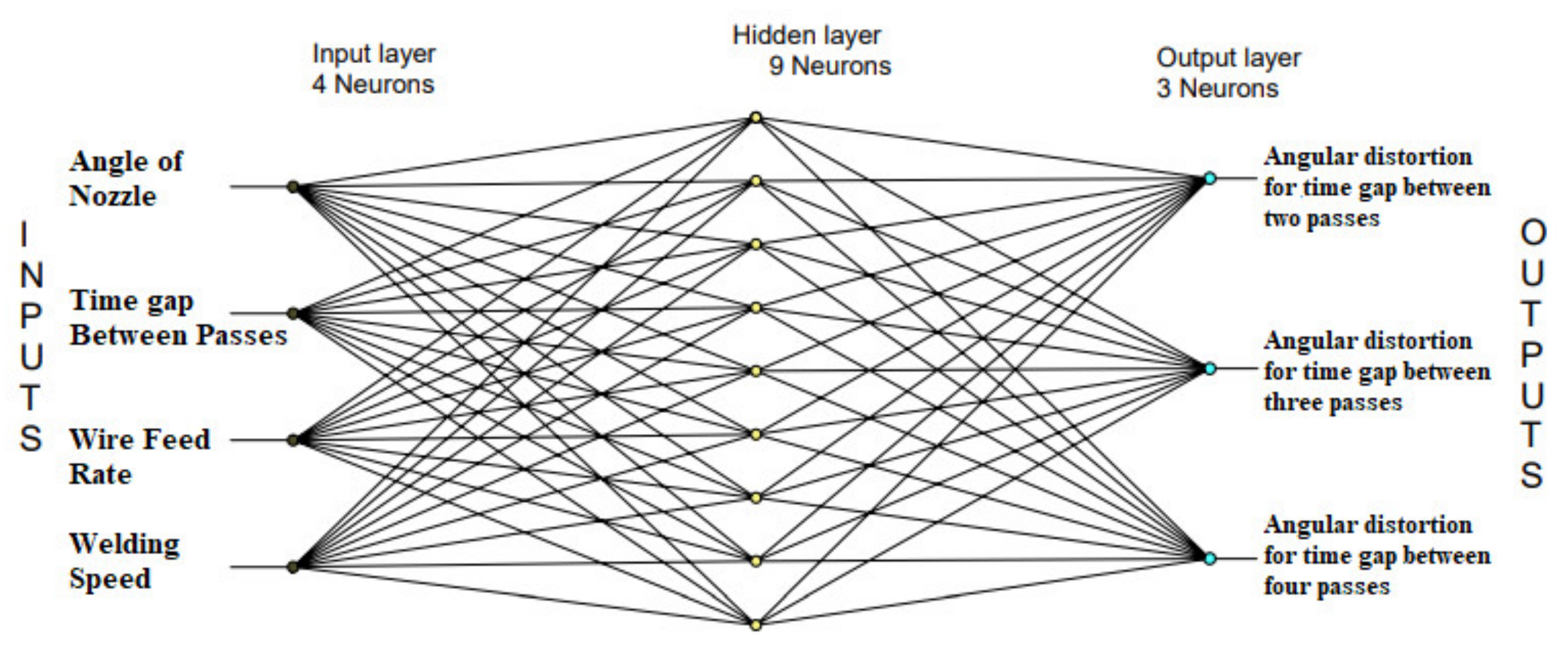
5. Neural Network Model Development
5.1. Neural Network Model Development
5.2. Network Training
- Xi = Normalized input/output value
- Zi = Actual input/output value
- Zmax = Maximum input/output value
- Zmin = Minimum input/output value
5.3. Testing the Network
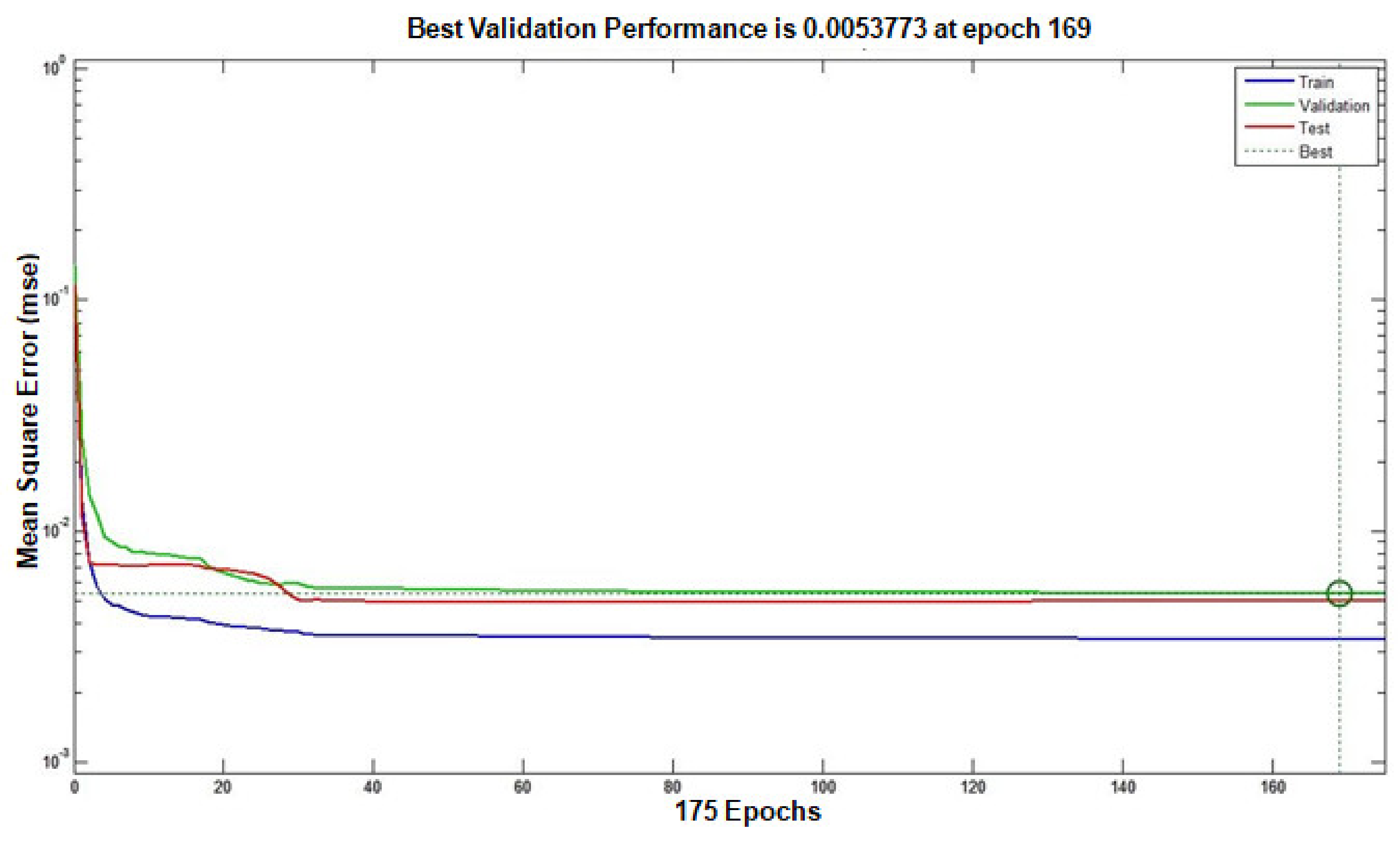
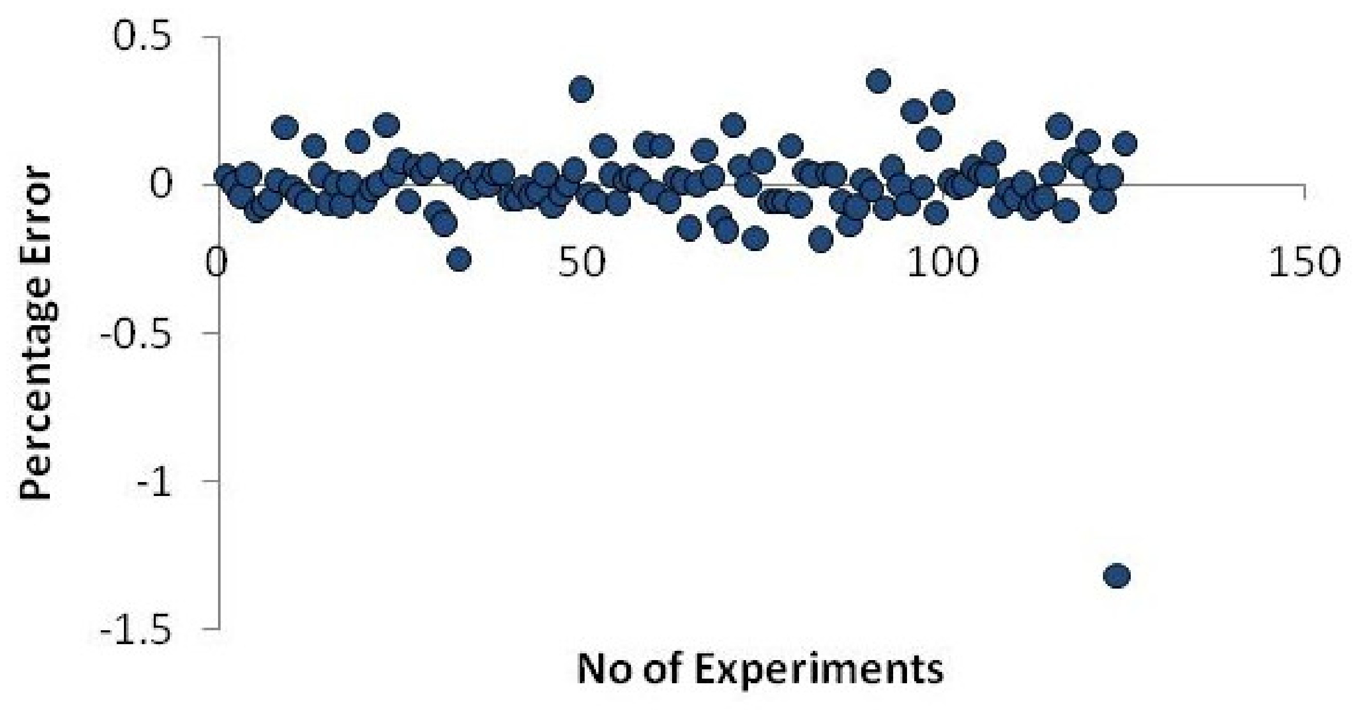
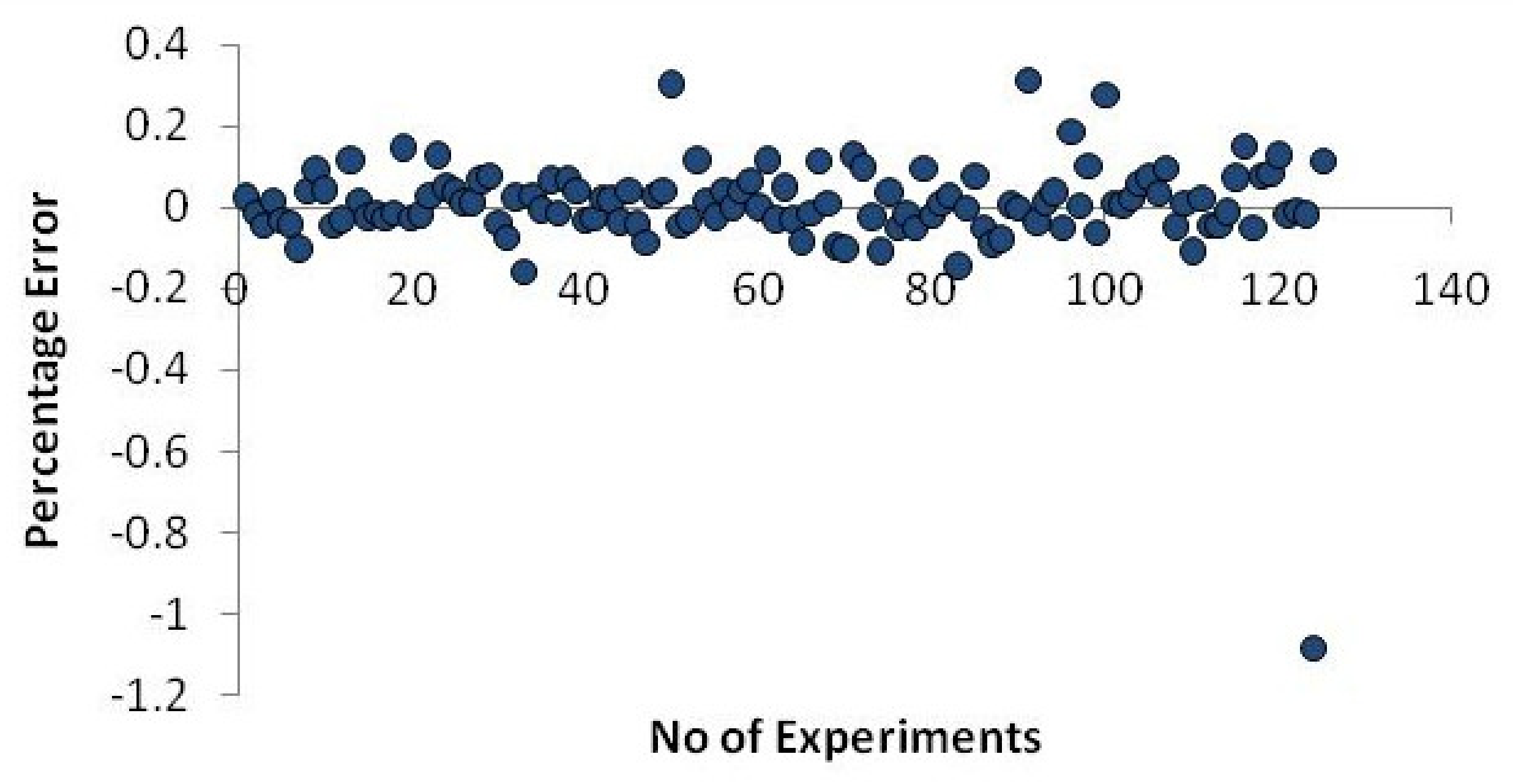
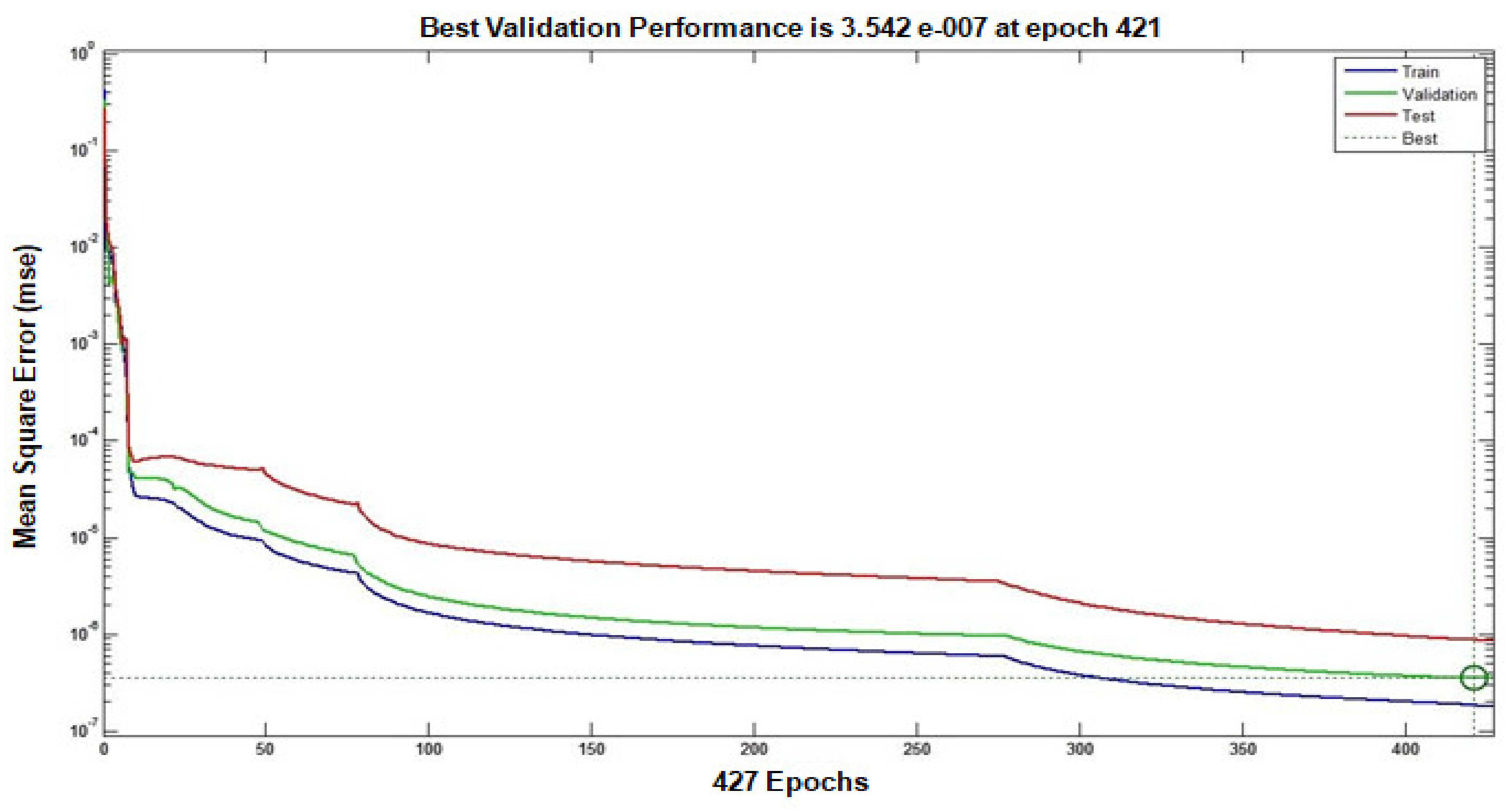
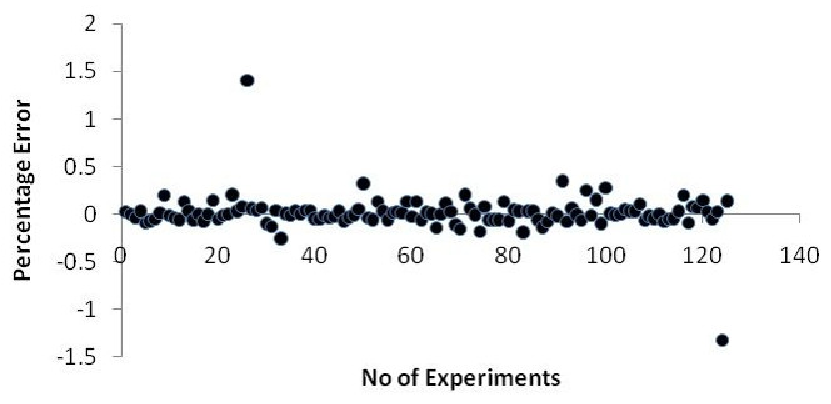
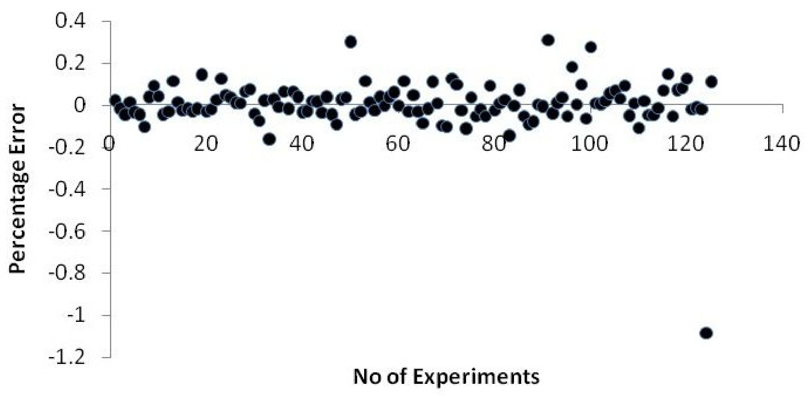
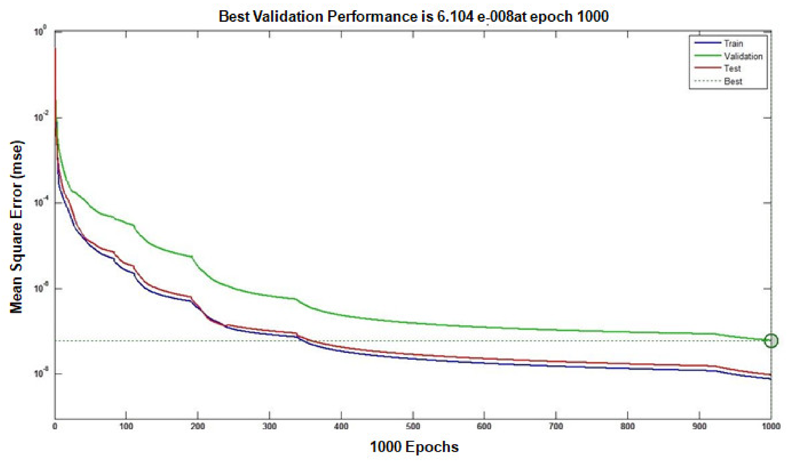
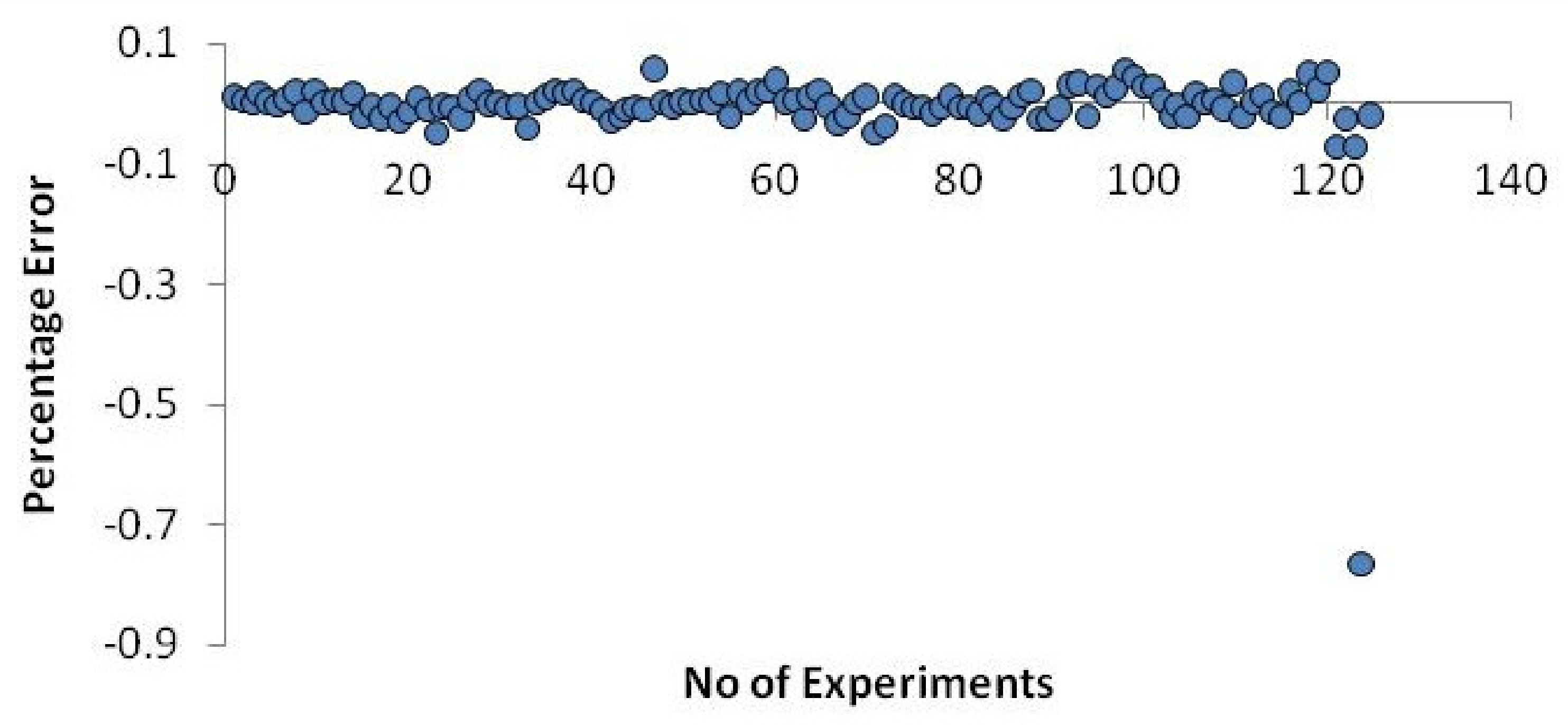
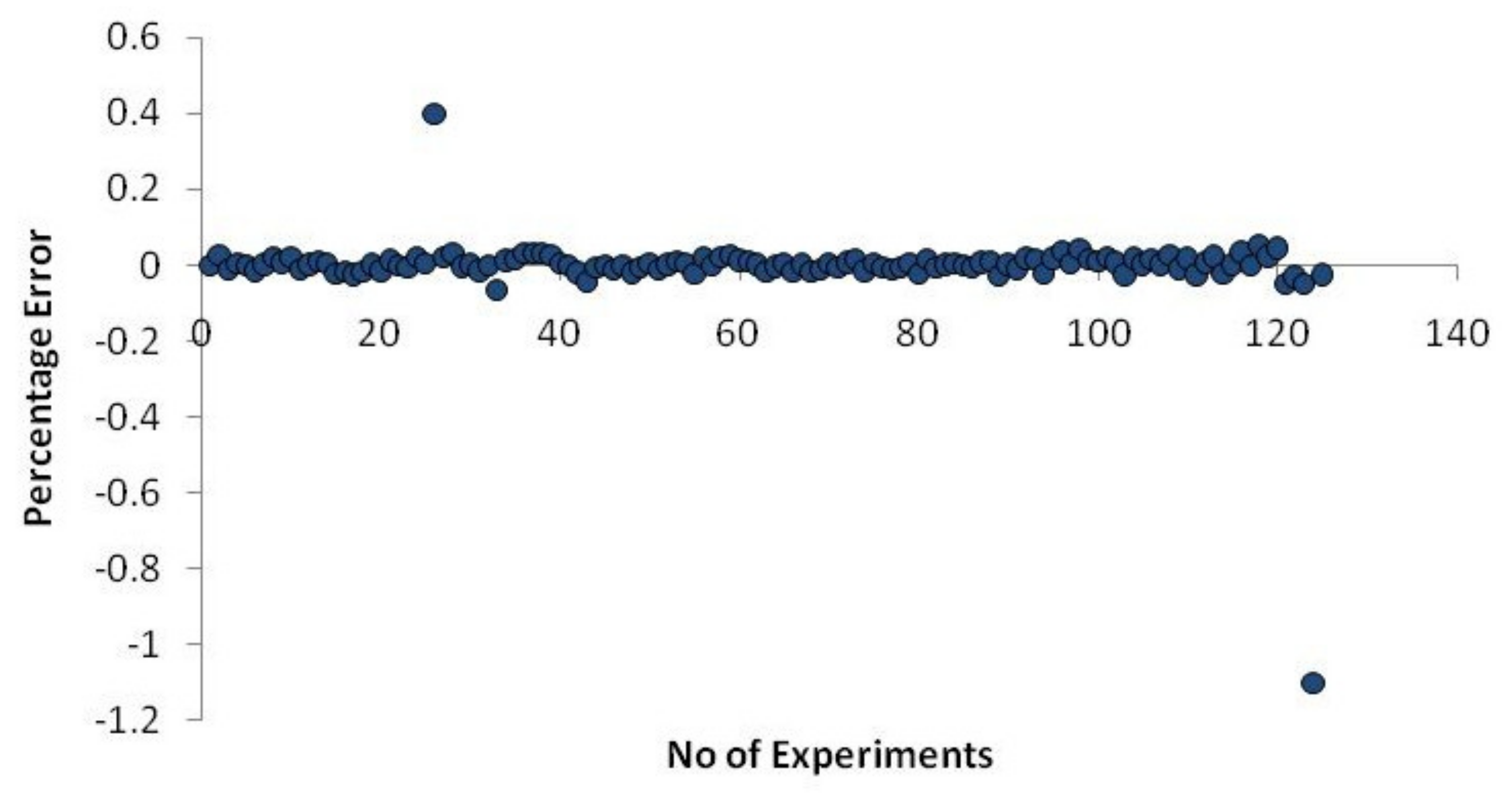
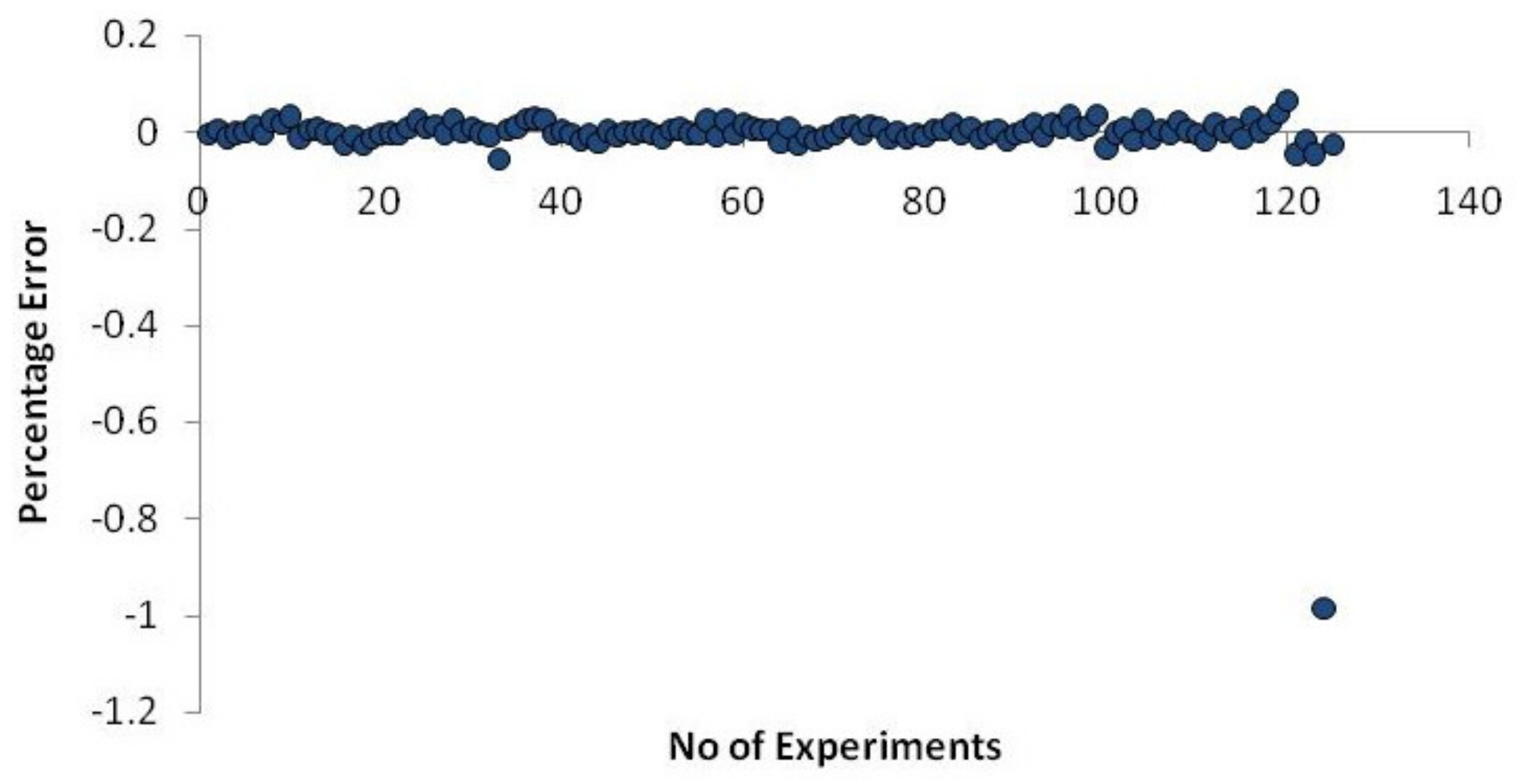
5.4. Network Analysis
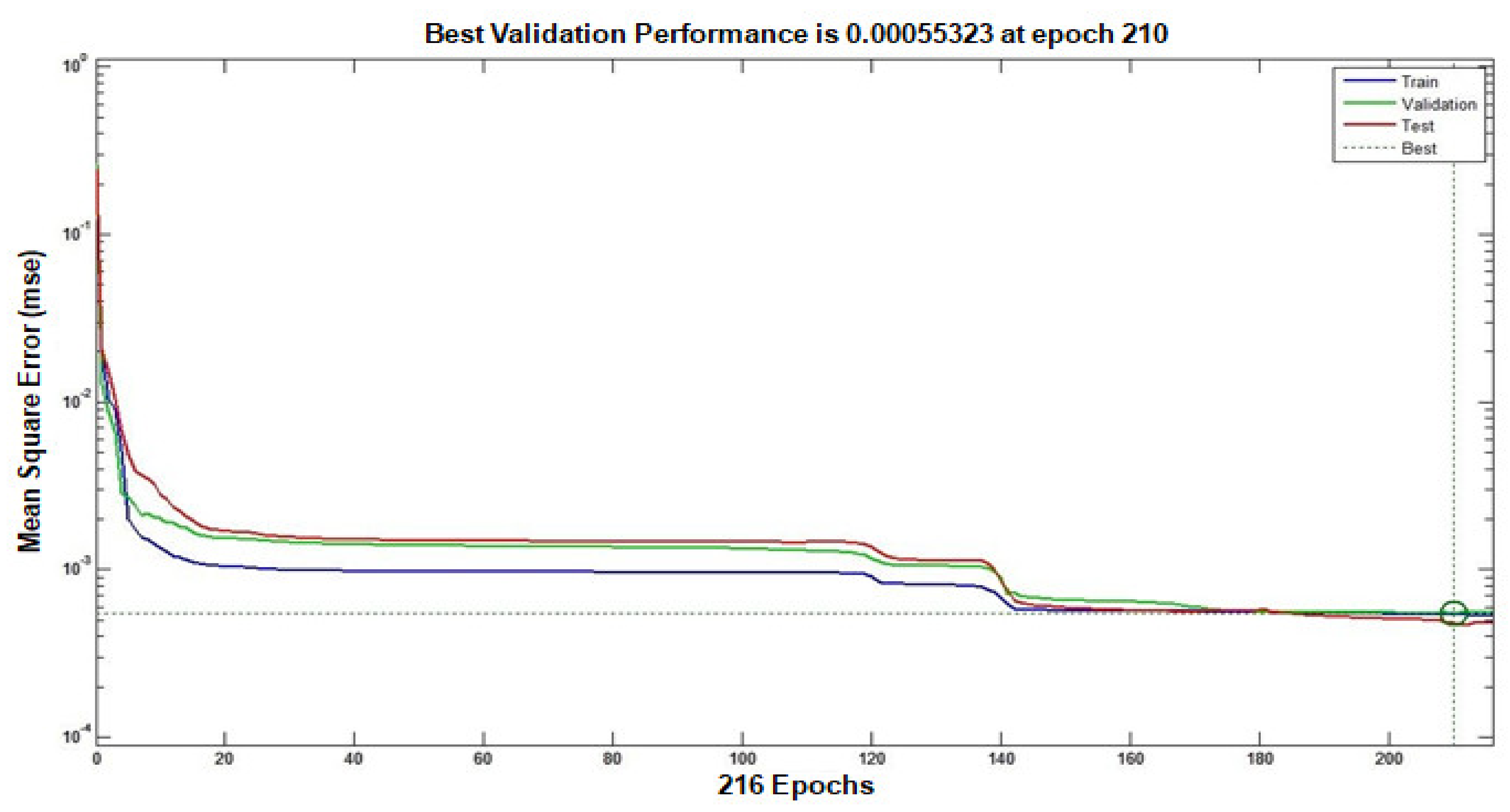
- Performance analysis
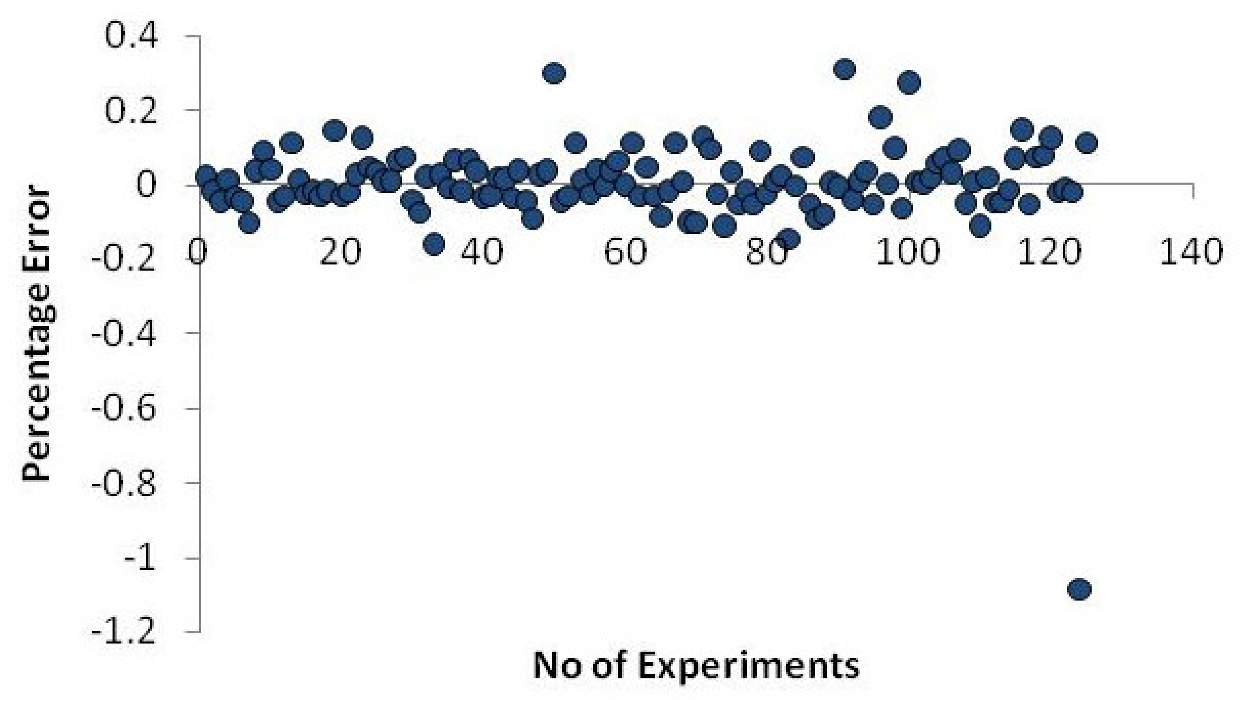
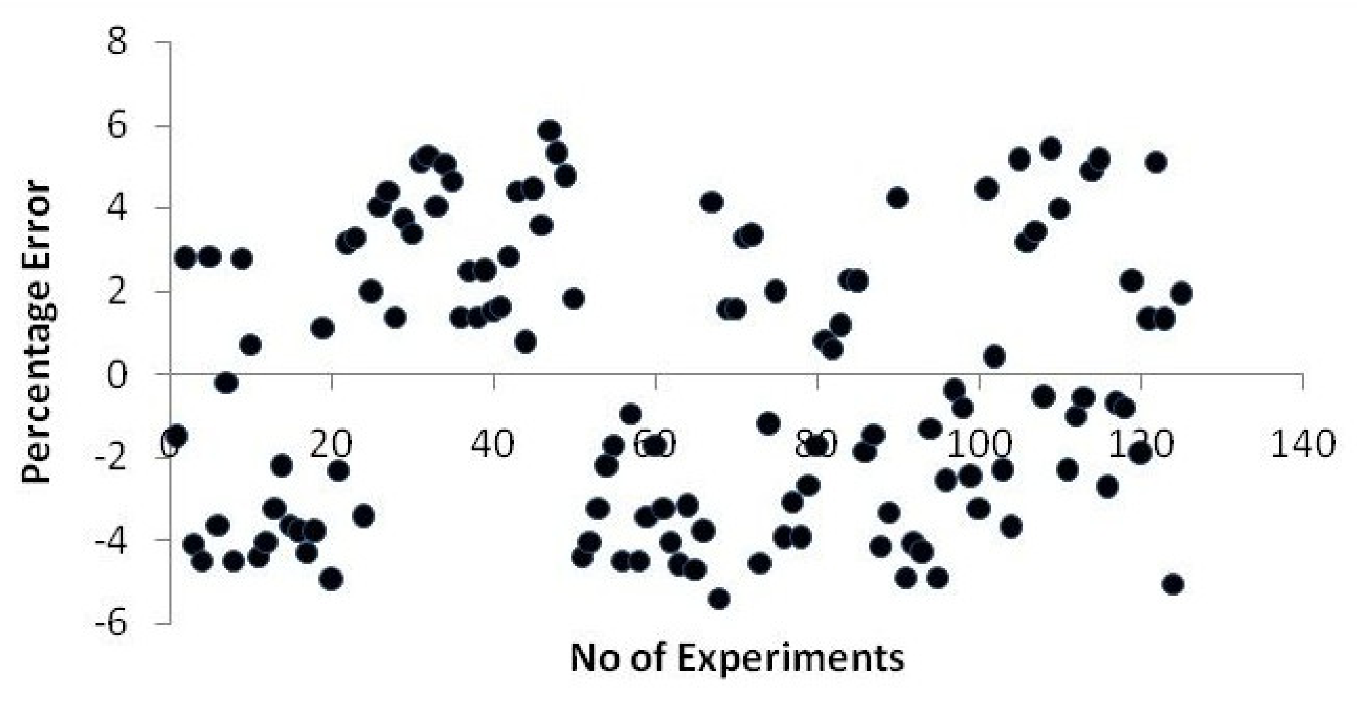
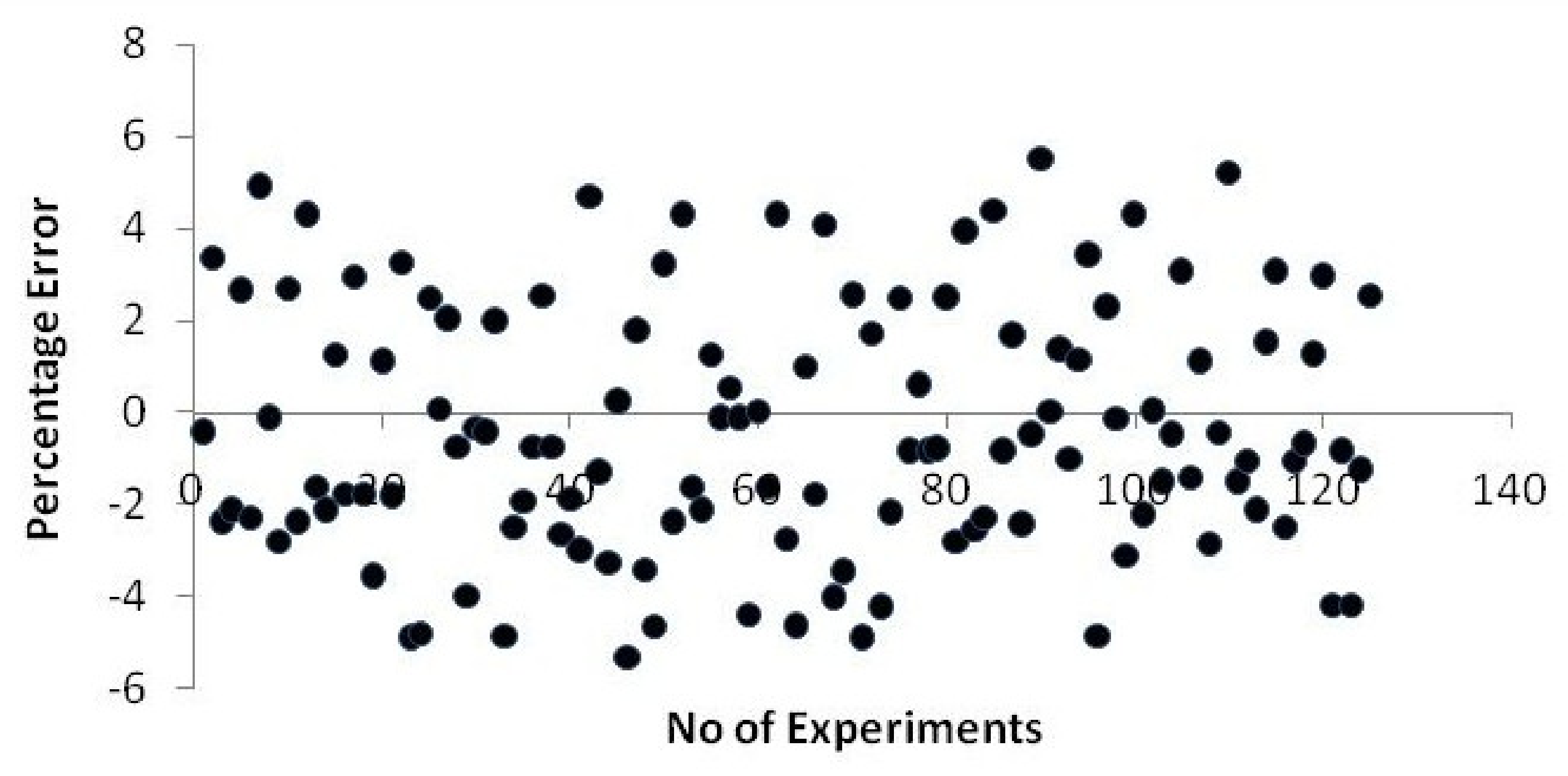
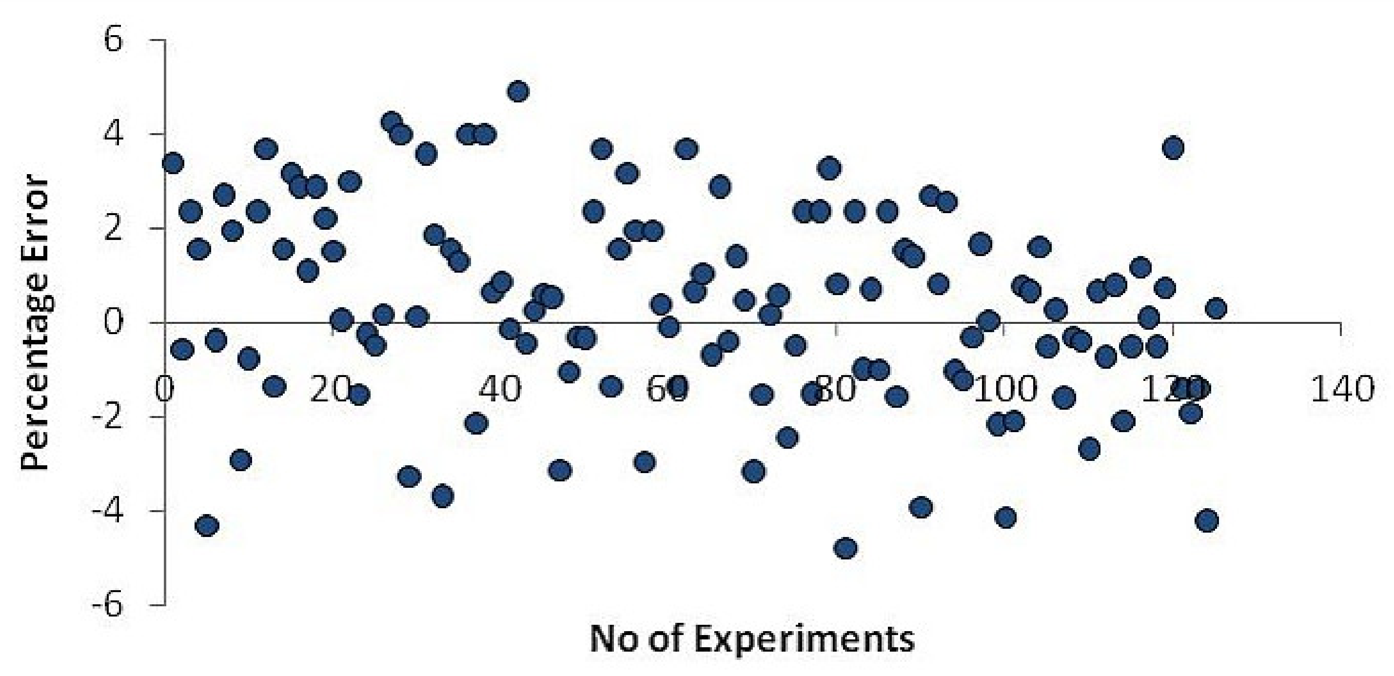
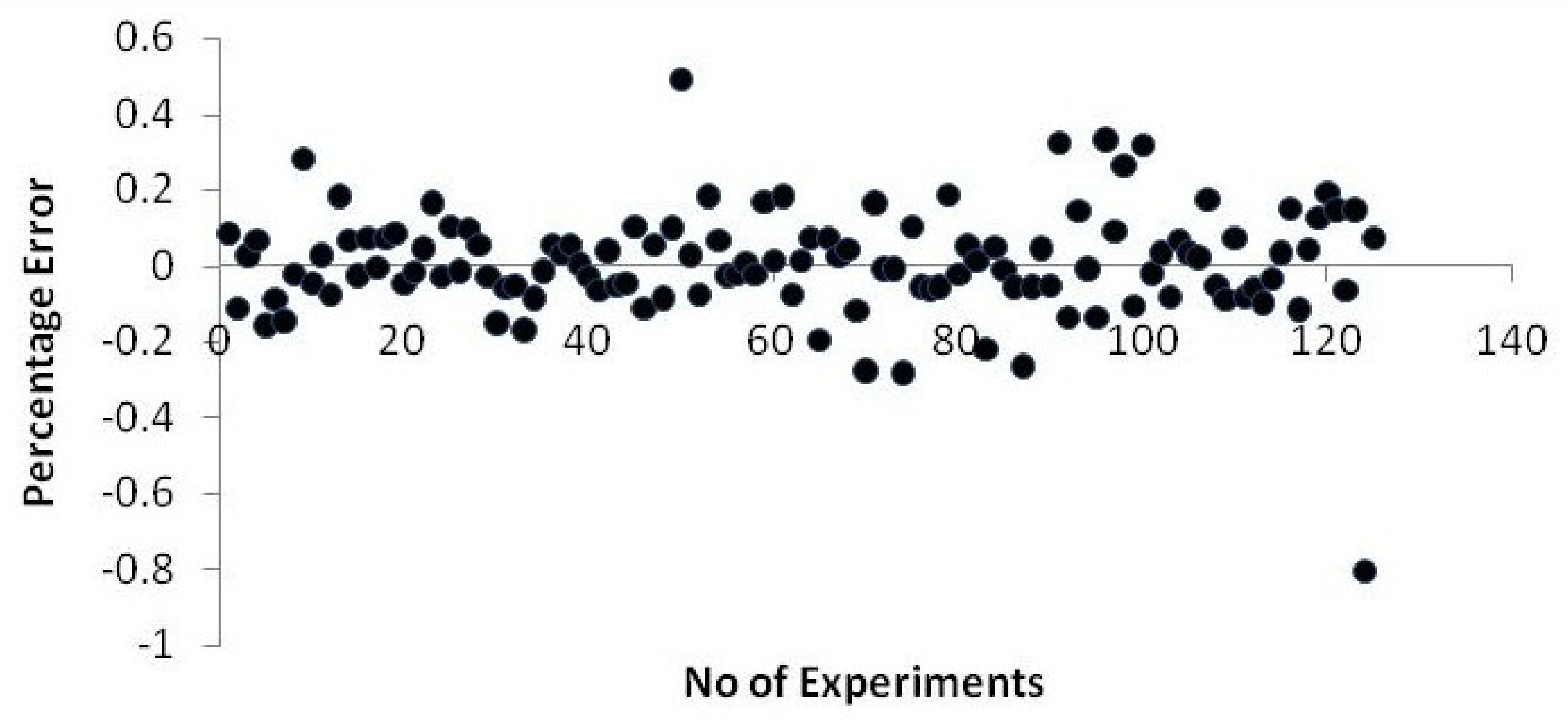
- Error analysis
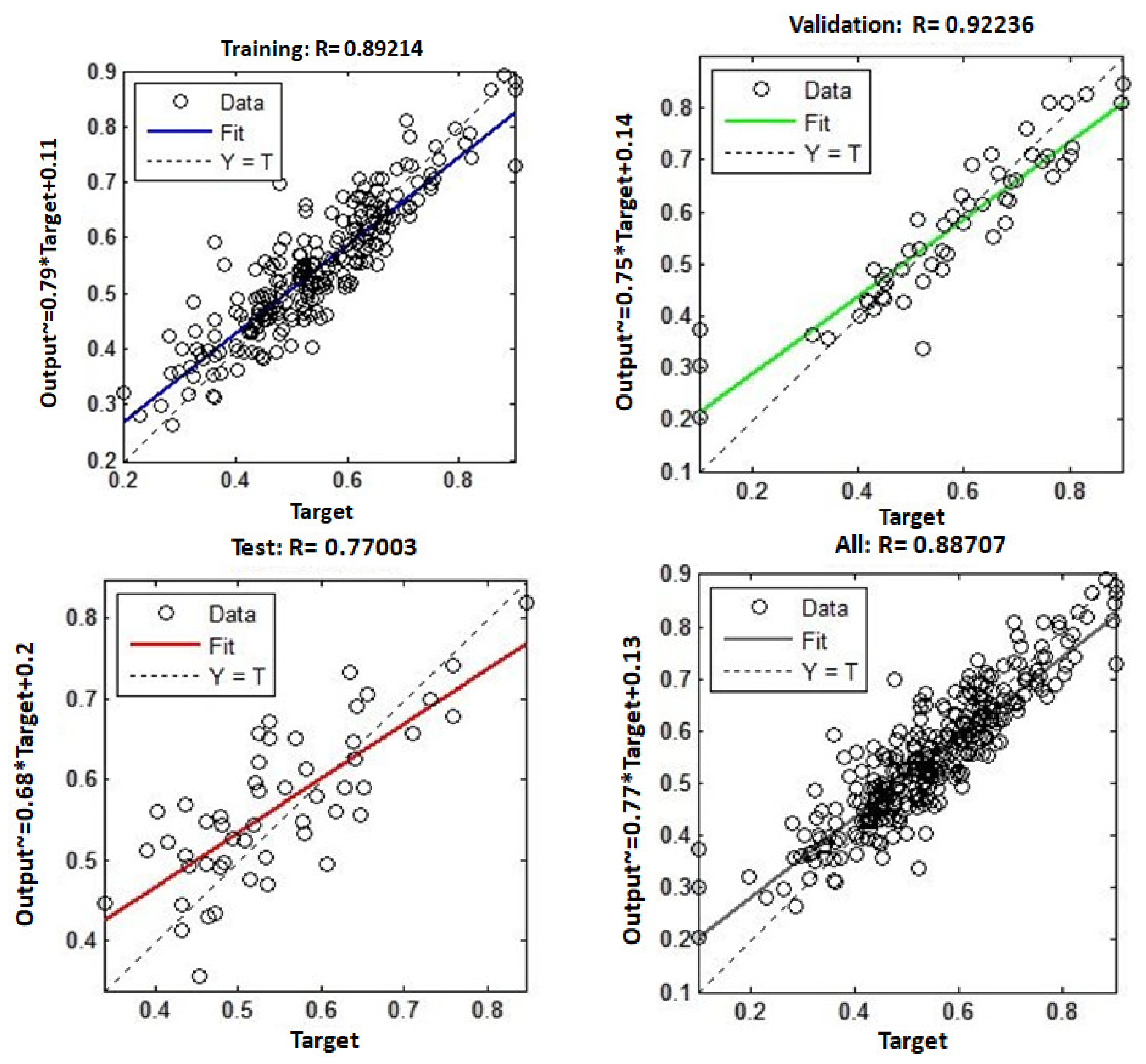
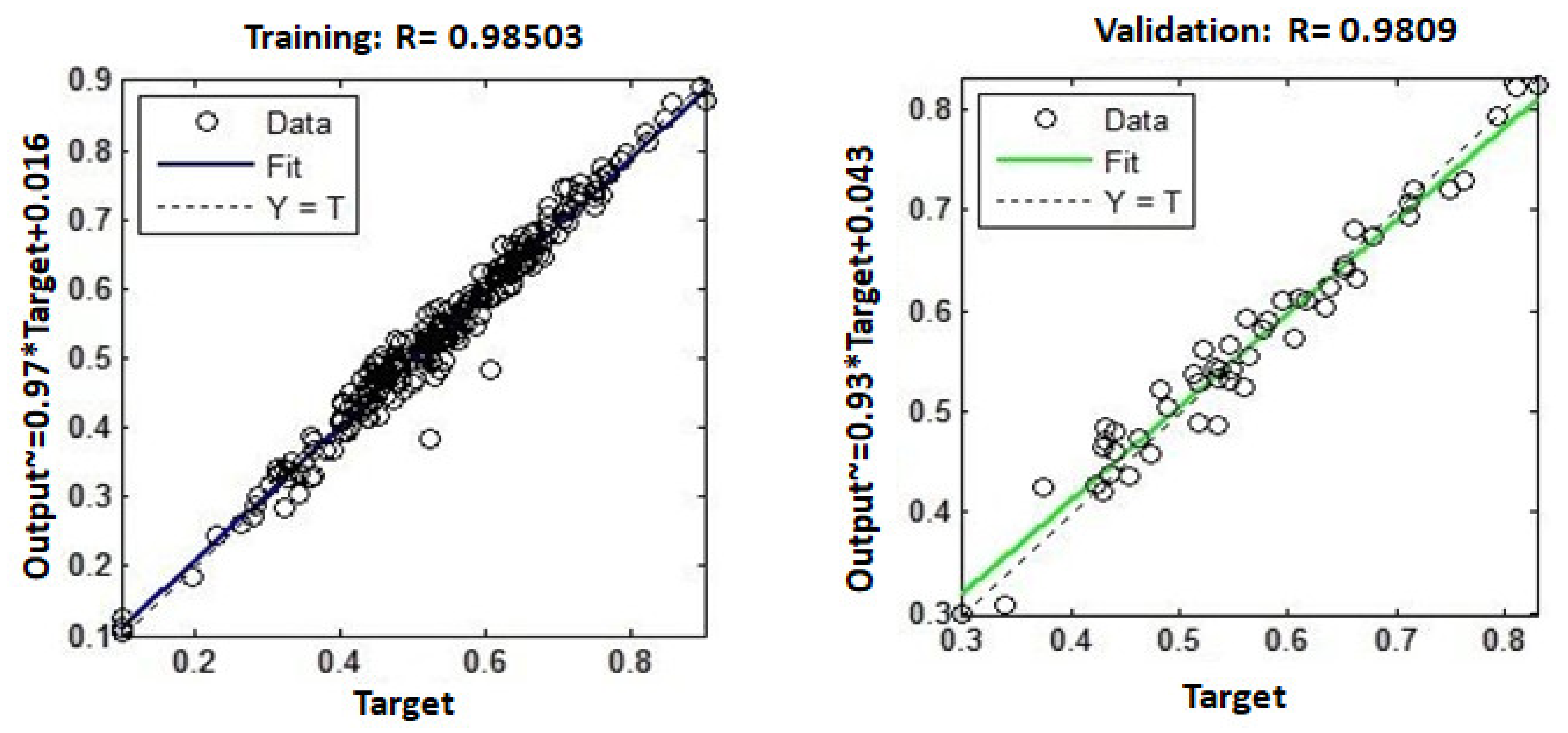
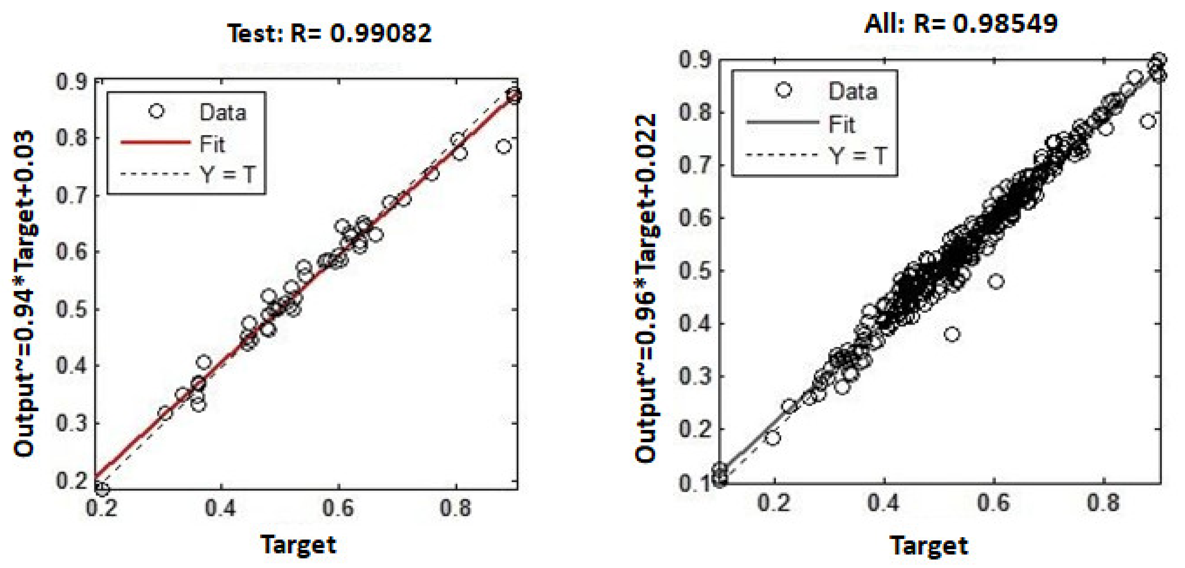
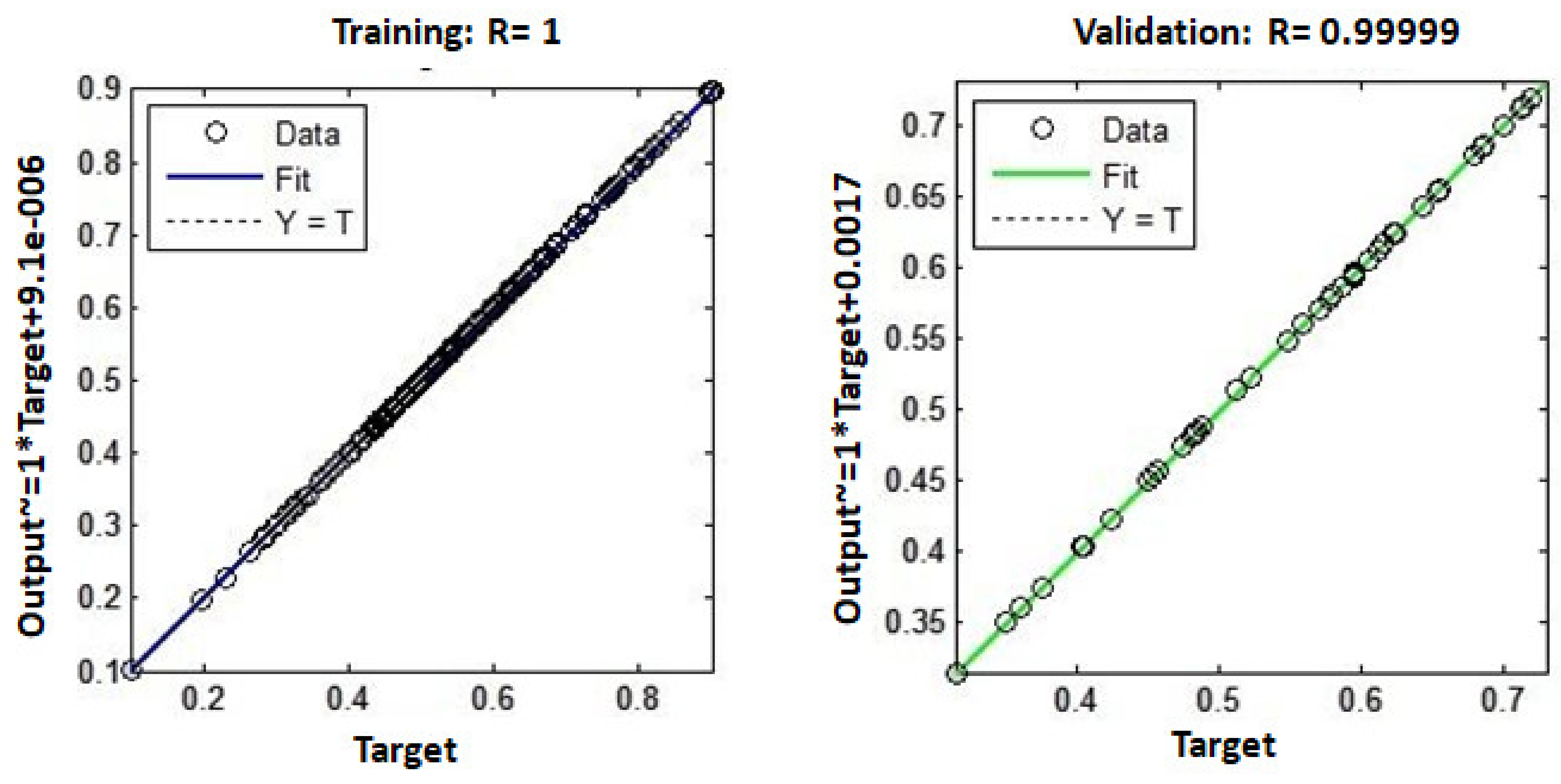
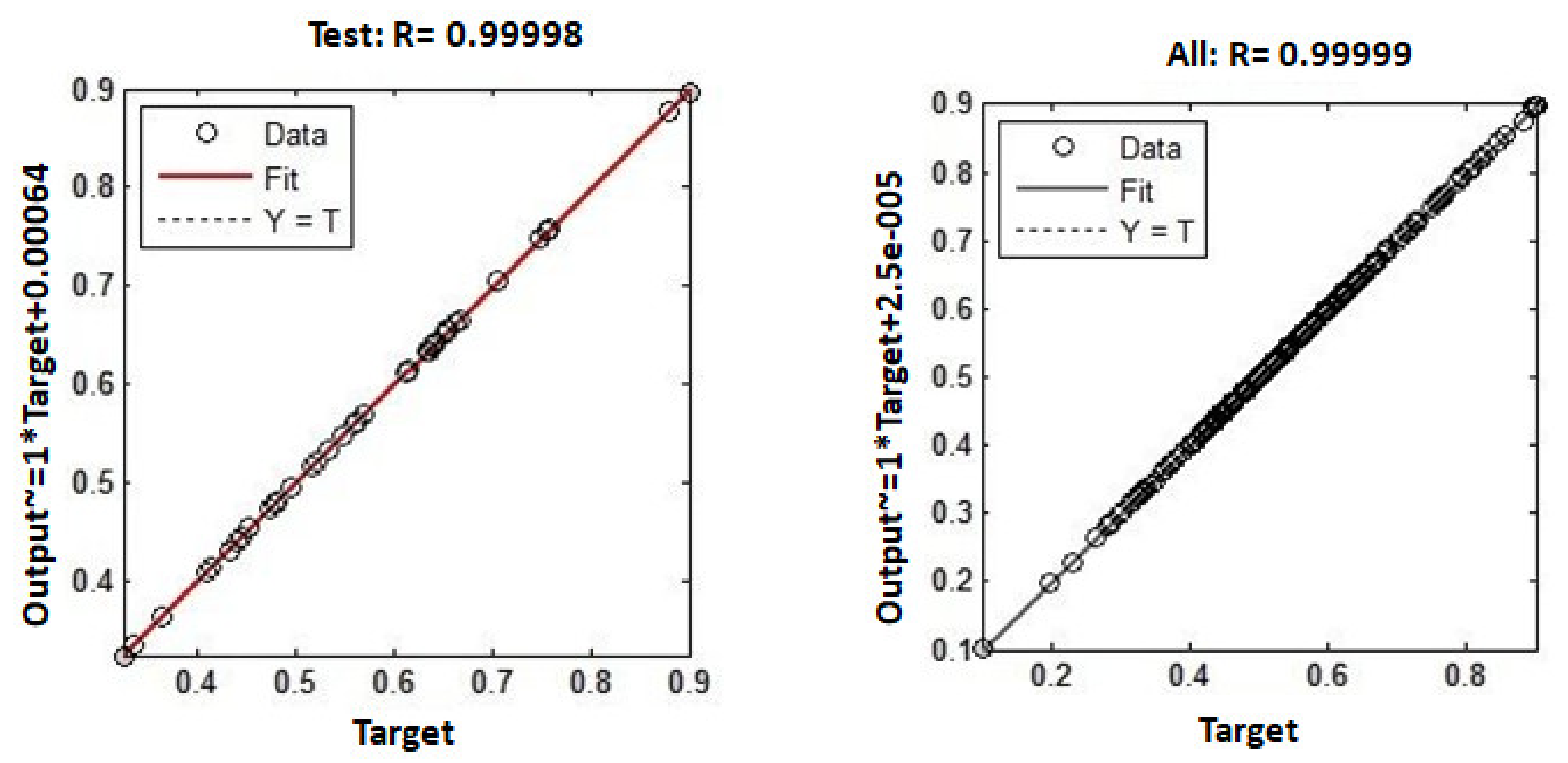
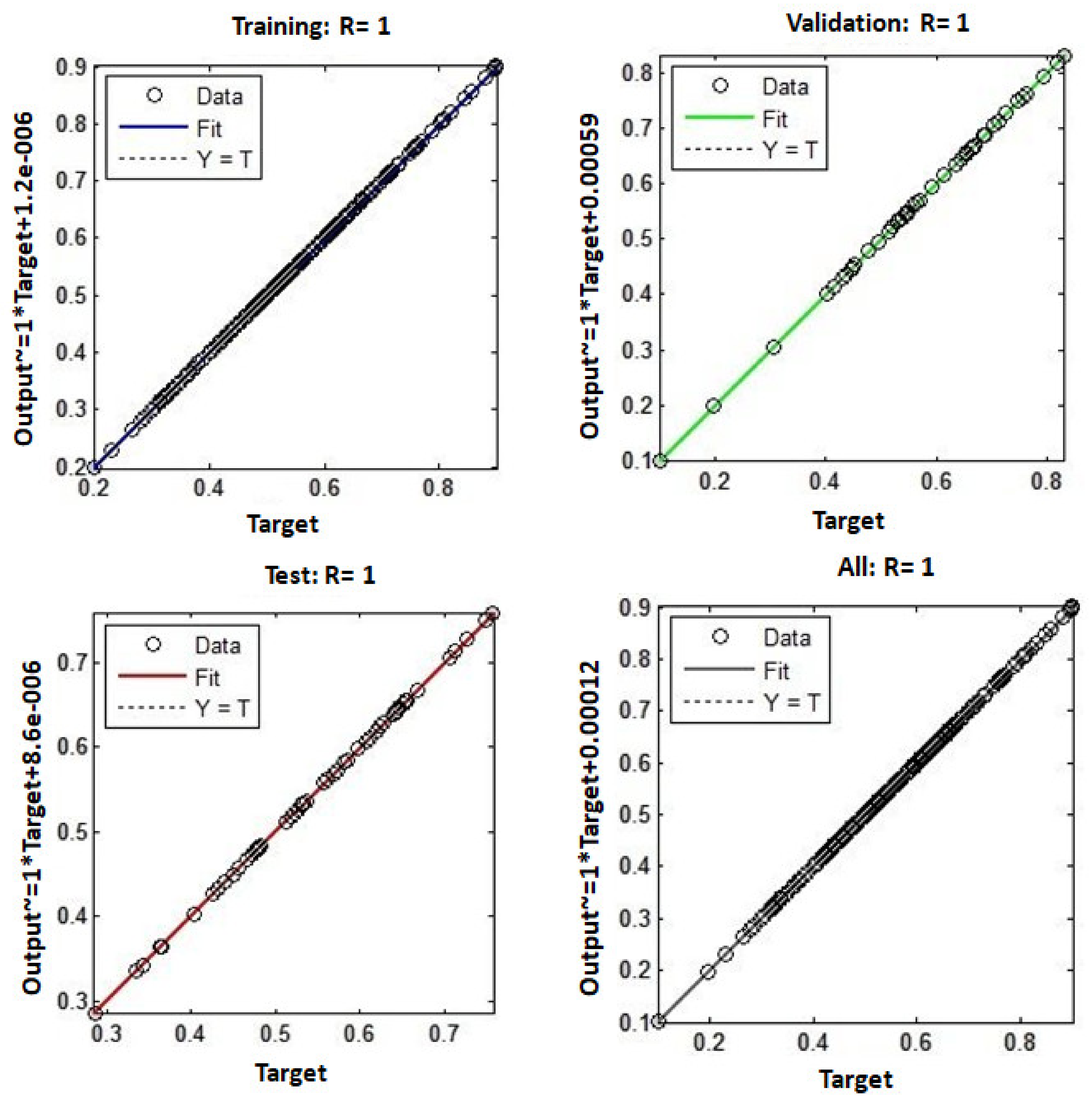
- Regression analysis
6. Confirmation of Results and Discussion
7. Conclusions
- In the gas metal arc welding technique, the structural steel studied in this work had good weld quality to achieve products of high quality. The products obtained from the GMAW of structural steel plate meets the required strength and free from angular distortion, which are the good weld quality criteria. As a result, it can be used in residential, commercial, and aviation hangar construction, as well as for construction purposes in metro stations, stadiums, and bridges.
- The fractional factorial-based 125 experimental runs were successful in collecting the data needed to create a neural network model.
- Validation experiments were carried out to ensure the network’s accuracy in forecasting angular distortion. The mean error for angular distortion with time gaps of two, three, and four passes was determined to be 0.92 percent, 0.20 percent, and 0.79 percent, respectively. This indicates that the model based on network 4-9-3 is more effective in forecasting angular distortion with time gaps between two, three, and four passes than the other three networks (4-2-3, 4-4-3, and 4-8-3). Prediction accuracy is more than 95 percent.
- The result shows that for training data, testing data, validation data, and all data, a correlation coefficient of R = 1 was found. Henceforth, there exists a good correlation between the observed and the predicted models.
- According to the study, different angular distortion values can be predicted by varying the hidden layer’s node count and applying a similar training method. The butt weld plate production process can be controlled using the neural network model developed in this paper to achieve the desired weld quality.
- The neural network model developed in this study can be used to manage the welding cycle in structural steel weld plates to achieve the best possible weld quality with the least amount of angular distortion.
- It is possible to develop a neural model for the prediction of angular distortion in thinner materials. As far as thinner materials are concerned, the gas tungsten arc welding process will be more appropriate because GTAW welds are preferable for thinner metals because they result in accurate and clean welds. Larger jobs requiring longer, continuous runs and thick metals respond well to GMAW welding.
Author Contributions
Funding
Data Availability Statement
Conflicts of Interest
References
- Shen, J.; Gonçalves, R.; Choi, Y.T.; Lopes, J.G.; Yang, J.; Schell, N.; Kim, H.S.; Oliveira, J.P. Microstructure and mechanical properties of gas metal arc welded CoCrFeMnNi joints using a 410 stainless steel filler metal. Mater. Sci. Eng. A 2022, 857, 144025. [Google Scholar] [CrossRef]
- Shen, J.; Gonçalves, R.; Choi, Y.T.; Lopes, J.G.; Yang, J.; Schell, N.; Kim, H.S.; Oliveira, J.P. Microstructure and mechanical properties of gas metal arc welded CoCrFeMnNi joints using a 308 stainless steel filler metal. Scr. Mater. 2023, 222, 115053. [Google Scholar] [CrossRef]
- Shen, J.; Agrawal, P.; Rodrigues, T.A.; Lopes, J.G.; Schell, N.; He, J.; Zeng, Z.; Mishra, R.S.; Oliveira, J.P.; Shen, J.; et al. Microstructure evolution and mechanical properties in a gas tungsten arc welded Fe42Mn28Co10Cr15Si5 metastable high entropy alloy. Mater. Sci. Eng. A 2023, 867, 144722. [Google Scholar] [CrossRef]
- Masubuchi, K. Analysis of Welded Structures; Pergamon Press: Oxford, UK, 1986. [Google Scholar] [CrossRef]
- Choobi, M.S.; Haghpanahi, M.; Sedighi, M. Prediction of welding-induced angular distortions in thin butt-welded plates using artificial neural networks. Comput. Mater. Sci. 2012, 62, 152–159. [Google Scholar] [CrossRef]
- Adamczuk, P.C.; Machado, I.G.; Mazzaferro, J.A.E. Methodology for predicting the angular distortion in multi-pass butt-joint welding. J. Mater. Process. Technol. 2017, 240, 305–313. [Google Scholar] [CrossRef]
- Kadir, M.H.A.; Asmelash, M.; Azhari, A. Investigation on welding distortion in stainless steel sheet using gas tungsten arc welding process. Mater. Today Proc. 2021, 46, 1674–1679. [Google Scholar] [CrossRef]
- Seong, W.J. Prediction and Characteristics of Angular Distortion in Multi-Layer Butt Welding. Materials 2019, 12, 1435. [Google Scholar] [CrossRef]
- Ansaripour, N.; Heidari, A.; Eftekhari, S.A. Multi-objective optimization of residual stresses and distortion in submerged arc welding process using genetic algorithm and harmony search. Proc. Inst. Mech. Eng. C J. 2020, 234, 862–871. [Google Scholar] [CrossRef]
- Vishvesha, A.; Pandey, C.; Mahapatra, M.M.; Mulik, R.S. On the estimation and control of welding distortion of guide blade carrier for a 660 MW turbine by using inherent strain method. Int. J. Steel Struct. 2017, 17, 53–63. [Google Scholar] [CrossRef]
- Wu, C.; Wang, C.; Lee, C.; Kim, J.W. An algorithm for prediction of bending deformation induced by multi-seam welding of a steel-pipe structure. J. Mech. Sci. Technol. 2021, 35, 707–716. [Google Scholar] [CrossRef]
- Zubairuddin, M.; Albert, S.K.; Mahadevan, S.; Vasudevan, M.; Chaudhari, V.; Suri, V.K. Experimental and finite element analysis of residual stress and distortion in GTA welding of modified 9Cr-1Mo steel. J. Mech. Sci. Technol. 2014, 28, 5095–5105. [Google Scholar] [CrossRef]
- Venkatesan, M.V.; Murugan, N.; Prasad, B.M.; Manickavasagam, A. Influence of FCA welding process parameters on distortion of 409m stainless steel for rail coach building. J. Iron Steel Res. Int. 2013, 20, 71–78. [Google Scholar] [CrossRef]
- Suman, S.; Sridhar, P.V.S.S.; Biswas, P.; Das, D. Prediction of welding-induced distortions in large weld structure through improved equivalent load method based on average plastic strains. Weld. World 2020, 64, 179–200. [Google Scholar] [CrossRef]
- Rong, Y.; Zhang, G.; Huang, Y. Study of welding distortion and residual stress considering nonlinear yield stress curves and multi-constraint equations. J. Mater. Eng. Perform. J. 2016, 25, 4484–4494. [Google Scholar] [CrossRef]
- Wang, C.; Kim, J.W. Numerical analysis of distortions by using an incorporated model for welding-heating-cutting processes of a welded lifting lug. J. Mech. Sci. Technol. 2018, 32, 5855–5862. [Google Scholar] [CrossRef]
- Chaki, S. Neural networks based prediction modeling of hybrid laser beam welding process parameters with sensitivity analysis. Appl. Sci. 2019, 1, 1285. [Google Scholar]
- Sudhakaran, R.; Sivasakthivel, P.S.; Subramanian, M.; Mahendran, S. Prediction of angular distortion in gas tungsten arc welded 202 grade stainless steel plates using artificial neural networks–An experimental approach. In AIP Conference Proceedings; AIP Publishing LLC: Melville, NY, USA, 2019; Volume 2161, p. 020050. [Google Scholar]
- Pazooki, A.M.A.; Hermans, M.J.M.; Richardson, I.M. Control of welding distortion during gas metal arc welding of AH36 plates by stress engineering. Int. J. Adv. Manuf. Technol. 2017, 88, 1439–1457. [Google Scholar] [CrossRef]
- Barclay, C.J.; Campbell, S.W.; Galloway, A.M.; McPherson, N.A. Artificial neural network prediction of weld distortion rectification using a travelling induction coil. Int. J. Adv. Manuf. Techn. 2013, 68, 127–140. [Google Scholar] [CrossRef]
- Tian, L.; Luo, Y.; Wang, Y.; Wu, X. Prediction of transverse and angular distortions of gas tungsten arc bead-on-plate welding using artificial neural network. Mater. Des. 2014, 54, 458–472. [Google Scholar] [CrossRef]
- Rubio-Ramirez, C.; Giarollo, D.F.; Mazzaferro, J.E.; Mazzaferro, C.P. Prediction of angular distortion due GMAW process of thin-sheets Hardox 450® steel by numerical model and artificial neural network. J. Manuf. Process. 2021, 68, 1202–1213. [Google Scholar] [CrossRef]
- Banik, S.D.; Kumar, S.; Singh, P.K.; Bhattacharya, S.; Mahapatra, M.M. Distortion and residual stresses in thick plate weld joint of austenitic stainless steel: Experiments and analysis. J. Mater. Process. Technol. 2021, 289, 6944. [Google Scholar] [CrossRef]
- Khoshroyan, A.; Darvazi, A.R. Effects of welding parameters and welding sequence on residual stress and distortion in Al6061-T6 aluminum alloy for T-shaped welded joint. Trans. Nonferrous Met. Soc. China 2020, 30, 76–89. [Google Scholar] [CrossRef]
- García-García, V.; Mejía, I.; Reyes-Calderón, F.; Benito, J.A.; Cabrera, J.M. FE thermo-mechanical simulation of welding residual stresses and distortion in Ti-containing TWIP steel through GTAW process. J. Manuf. Process. 2020, 59, 801–815. [Google Scholar] [CrossRef]
- Venkatkumar, D.; Ravindran, D.; Selvakumar, G. Finite element analysis of heat input effect on temperature, residual stresses and distortion in butt welded plates. Mater. Today Proc. 2018, 5, 8328–8337. [Google Scholar] [CrossRef]
- Vasantharaja, P.; Vasudevan, M.; Palanichamy, P. Effect of welding processes on the residual stress and distortion in type 316LN stainless steel weld joints. J. Manuf. Process. 2015, 19, 187–193. [Google Scholar] [CrossRef]
- Bajpei, T.; Chelladurai, H.; Ansari, M.Z. Experimental investigation and numerical analyses of residual stresses and distortions in GMA welding of thin dissimilar AA5052-AA6061 plates. J. Manuf. Process. 2017, 25, 340–350. [Google Scholar] [CrossRef]
- Laksha; Bharti, P.; Khanna, P. Prediction of angular distortion in MIG welding of stainless steel 202 plates. In Advances in Mechanical and Materials Technology: Select Proceedings of EMSME; Springer: Singapore, 2022; pp. 525–536. [Google Scholar]
- Lohate, M.S.; Damale, A.V. Fuzzy based prediction of angular distortion of gas metal arc welded structural steel plates. Int. J. Innov. 2015, 2394–3696. [Google Scholar]
- Baskoro, A.S.; Hidayat, R.; Widyianto, A.; Amat, M.A.; Putra, D.U. Optimization of Gas Metal Arc Welding (GMAW) parameters for minimum distortion of t welded joints of A36 mild steel by Taguchi method. Mater. Sci. Forum 2020, 1000, 356–363. [Google Scholar] [CrossRef]
- Xie, D.; Zhao, J.; Liang, H.; Liu, S.; Tian, Z.; Shen, L.; Wang, C. Cause of angular distortion in fusion welding: Asymmetric cross-sectional profile along thickness. Materials 2019, 12, 58. [Google Scholar] [CrossRef]
- Yu, R.; Zhao, Z.; Bai, L.; Han, J. Prediction of weld reinforcement based on vision sensing in GMA additive manufacturing process. Metals 2020, 10, 1041. [Google Scholar] [CrossRef]
- Cochran, W.G.; Cox, G.M. Experimental Designs, 2nd ed.; Wiley: Hoboken, NJ, USA, 1992. [Google Scholar]
- Sudhakaran, R.; VeL Murugan, V.; Senthil Kumar, K.M.; Jayaram, R.; Pushparaj, A.; Praveen, C.; Venkat Prabhu, N. Effect of welding parameters on weld bead geometry and optimization of process parameters to maximize depth to width ratio for stainless steel gas tungsten arc welded plates using genetic algorithm. Eur. J. Sci. Res. 2011, 62, 76–94. [Google Scholar]
- Shim, J.Y.; Zhang, J.W.; Yoon, H.Y.; Kang, B.Y.; Kim, I.S. Prediction model for bead reinforcement area in automatic gas metal arc welding. Adv. Mech. Eng. 2018, 10, 1687814018781492. [Google Scholar] [CrossRef]
- Zain, A.M.; Haron, H.; Sharif, S. Prediction of surface roughness in the end milling machining using artificial neural network. Expert Syst. Appl. 2010, 37, 1755–1768. [Google Scholar] [CrossRef]
- Narayanareddy, V.V.; Chandrasekhar, N.; Vasudevan, M.; Muthukumaran, S.; Vasantharaja, P. Numerical simulation and artificial neural network modeling for predicting welding-induced distortion in butt-welded 304L stainless steel plates. Metall. Mater. Trans. B 2016, 47, 702–713. [Google Scholar] [CrossRef]
- Li, Y.; Lee, T.H.; Wang, C.; Wang, K.; Tan, C.; Banu, M.; Hu, S.J. An artificial neural network model for predicting joint performance in ultrasonic welding of composites. Procedia CIRP 2018, 76, 85–88. [Google Scholar] [CrossRef]
- Jacques, L.; El Ouafi, A. ANN based predictive modeling of weld shape and dimensions in laser welding of galvanized steel in butt joint configurations. JMMCE 2018, 6, 316. [Google Scholar] [CrossRef]
- Oussaid, K.; El Ouafi, A. A study on prediction of weld geometry in laser overlap welding of low carbon galvanized steel using ANN-based models. J. Softw. Eng. Appl. 2019, 12, 509. [Google Scholar] [CrossRef]
- Saeed, M.M.; Al Sarraf, Z.S. Using artificial neural networks to predict the effect of input parameters on weld bead geometry for saw process. J. Eur. Syst. Autom. 2021, 54, 309–315. [Google Scholar] [CrossRef]
- Jacques, L.; El Ouafi, A. Prediction of Weld joint shape and dimensions in laser welding using a 3d modeling and experimental validation. Mater. Sci. Appl. 2017, 8, 757–773. [Google Scholar] [CrossRef]
- Zubairuddin, M.; Chaursaia, P.K.; Ali, B. Thermo-mechanical analysis of laser welding of Grade 91 steel plates. Optik 2021, 245, 167510. [Google Scholar] [CrossRef]
- Zubairuddin, M.; Albert, S.K.; Reddy, M.S.; Ali, B.; Varaprasad, B.; Mishra, A.; Das, P.K.; Elumalai, P.V. Thermal analysis of thin P91 steel using FlexPDE and SYSWELD. Mater. Today Proc. 2023, 72, 1550–1555. [Google Scholar] [CrossRef]
- Kumar, P.; Kumar, R.; Arif, A.; Veerababu, M. Investigation of numerical modelling of TIG welding of austenitic stainless steel (304L). Mater. Today Proc. 2020, 27, 1636–1640. [Google Scholar] [CrossRef]
- Afzal, A.; Aabid, A.; Khan, A.; Khan, S.A.; Rajak, U.; Verma, T.N.; Kumar, R. Response Surface Analysis, Clustering, and Random Forest Regression of Pressure in Suddenly Expanded High-Speed Aerodynamic Flows. Aerosp. Sci. Technol. 2020, 107, 106318. [Google Scholar] [CrossRef]
- Afzal, A.; Ansari, Z.; Faizabadi, A.R.; Ramis, M.K. Parallelization Strategies for Computational Fluid Dynamics Software: State of the Art Review. Arch. Comput. Methods Eng. 2017, 24, 337–363. [Google Scholar] [CrossRef]
- Afzal, A.; Abdul Mujeebu, M. Thermo-Mechanical and Structural Performances of Automobile Disc Brakes: A Review of Numerical and Experimental Studies. Arch. Comput. Methods Eng. 2019, 26, 1489–1513. [Google Scholar] [CrossRef]
- Pinto, R.N.; Afzal, A.; D’Souza, L.V.; Ansari, Z.; Mohammed Samee, A. Computational Fluid Dynamics in Turbomachinery: A Review of State of the Art. Arch. Comput. Methods Eng. 2017, 24, 467–479. [Google Scholar] [CrossRef]
- Jilte, R.; Afzal, A.; Panchal, S. A Novel Battery Thermal Management System Using Nano-Enhanced Phase Change Materials. Energy 2021, 219, 119564. [Google Scholar] [CrossRef]
- Ağbulut, Ü.; Sarıdemir, S.; Rajak, U.; Polat, F.; Afzal, A.; Verma, T.N. Effects of High-Dosage Copper Oxide Nanoparticles Addition in Diesel Fuel on Engine Characteristics. Energy 2021, 229, 120611. [Google Scholar] [CrossRef]
- Afzal, A.; Bhutto, J.K.; Alrobaian, A.; Kaladgi, A.R.; Khan, S.A. Modelling and Computational Experiment to Obtain Optimized Neural Network for Battery Thermal Management Data. Energies 2021, 14, 7370. [Google Scholar] [CrossRef]
- Mokashi, I.; Afzal, A.; Khan, S.A.; Abdullah, N.A.; Bin Azami, M.H.; Jilte, R.D.; Samuel, O.D. Nusselt Number Analysis from a Battery Pack Cooled by Different Fluids and Multiple Back-Propagation Modelling Using Feed-Forward Networks. Int. J. Therm. Sci. 2021, 161, 106738. [Google Scholar] [CrossRef]
- Chaluvaraju, B.V.; Afzal, A.; Vinnik, D.A.; Kaladgi, A.R.; Alamri, S.; Tirth, V. Mechanical and Corrosion Studies of Friction Stir Welded Nano Al2O3 Reinforced Al-Mg Matrix Composites: RSM-ANN Modelling Approach. Symmetry 2021, 13, 537. [Google Scholar] [CrossRef]
- Afzal, A.; Khan, S.A.; Salee, C.A. Role of Ultrasonication Duration and Surfactant on Characteristics of ZnO and CuO Nanofluids. Mater. Res. Express 2019, 6, 1150d8. [Google Scholar] [CrossRef]
- Afzal, A.; Nawfal, I.; Mahbubul, I.M.; Kumbar, S.S. An Overview on the Effect of Ultrasonication Duration on Different Properties of Nanofluids. J. Therm. Anal. Calorim. 2019, 135, 393–418. [Google Scholar] [CrossRef]
- Afzal, A.; Navid, K.M.Y.; Saidur, R.; Razak, R.K.A.; Subbiah, R. Back Propagation Modeling of Shear Stress and Viscosity of Aqueous Ionic - MXene Nanofluids. J. Therm. Anal. Calorim. 2021, 145, 2129–2149. [Google Scholar] [CrossRef]
- Bakır, H.; Ağbulut, Ü.; Gürel, A.E.; Yıldız, G.; Güvenç, U.; Soudagar, M.E.M.; Hoang, A.T.; Deepanraj, B.; Saini, G.; Afzal, A. Forecasting of Future Greenhouse Gas Emission Trajectory for India Using Energy and Economic Indexes with Various Metaheuristic Algorithms. J. Clean. Prod. 2022, 360, 131946. [Google Scholar] [CrossRef]
- David, O.; Waheed, M.A.; Taheri-Garavand, A.; Nath, T.; Dairo, O.U.; Bolaji, B.O.; Afzal, A. Prandtl Number of Optimum Biodiesel from Food Industrial Waste Oil and Diesel Fuel Blend for Diesel Engine. Fuel 2021, 285, 119049. [Google Scholar] [CrossRef]
- David, O.; Okwu, M.O.; Oyejide, O.J.; Taghinezhad, E.; Asif, A.; Kaveh, M. Optimizing Biodiesel Production from Abundant Waste Oils through Empirical Method and Grey Wolf Optimizer. Fuel 2020, 281, 118701. [Google Scholar] [CrossRef]
- Sharath, B.N.; Venkatesh, C.V.; Afzal, A. Multi Ceramic Particles Inclusion in the Aluminium Matrix and Wear Characterization through Experimental and Response Surface-Artificial Neural Networks. Materials 2021, 14, 2895. [Google Scholar] [CrossRef]
- Afzal, A.; Saleel, C.A.; Badruddin, I.A.; Khan, T.M.Y.; Kamangar, S.; Mallick, Z.; Samuel, O.D.; Soudagar, M.E.M. Human Thermal Comfort in Passenger Vehicles Using an Organic Phase Change Material–An Experimental Investigation, Neural Network Modelling, and Optimization. Build. Environ. 2020, 180, 107012. [Google Scholar] [CrossRef]
- Afzal, A.; Mokashi, I.; Khan, S.A.; Abdullah, N.A.; Azami, M.H.B. Optimization and Analysis of Maximum Temperature in a Battery Pack Affected by Low to High Prandtl Number Coolants Using Response Surface Methodology and Particle Swarm Optimization Algorithm. Numer. Heat Transf. Part A Appl. 2020, 79, 406–435. [Google Scholar] [CrossRef]
- Afzal, A.; Khan, S.A.; Islam, T.; Jilte, R.D.; Khan, A.; Soudagar, M.E.M. Investigation and Back-Propagation Modeling of Base Pressure at Sonic and Supersonic Mach Numbers. Phys. Fluids 2020, 32, 096109. [Google Scholar] [CrossRef]
- Sathish, T.; Kaladgi, A.R.R.; Mohanavel, V.; Arul, K.; Afzal, A.; Aabid, A. Experimental Investigation of the Friction Stir Weldability of AA8006 with Zirconia Particle Reinforcement and Optimized Process Parameters. Materials 2021, 14, 2782. [Google Scholar] [CrossRef] [PubMed]
- Afzal, A.; Samee, A.D.M.; Javad, A.; Shafvan, S.A.; Ajinas, P.V.; Kabeer, K.M.A. Heat Transfer Analysis of Plain and Dimpled Tubes with Different Spacings. Heat Transf. Res. 2018, 47, 556–568. [Google Scholar] [CrossRef]


| C% (Max) | Mn% (Max) | S% (Max) | P% (Max) | Si% (Max) | CE% (Max) |
|---|---|---|---|---|---|
| 0.23 | 1.50 | 0.050 | 0.050 | 0.40 | 0.42 |
| Process Parameters | Units | Notation | Limits | ||||
|---|---|---|---|---|---|---|---|
| −2 | −1 | 0 | +1 | +2 | |||
| Angle of electrode to work piece | Deg | θ | 70 | 80 | 90 | 100 | 110 |
| Time gap between passes | minutes | T | 5 | 10 | 15 | 20 | 25 |
| Wire feed rate | m/min | F | 5 | 5.25 | 5.5 | 5.75 | 6 |
| Welding speed | cm/min | S | 8.4 | 9 | 9.6 | 10.2 | 10.8 |
| S. No. | θ | T | F | S | α 2 Degrees | α 3 Degrees | α 4 Degrees |
|---|---|---|---|---|---|---|---|
| 1 | 0 | 0 | 0 | 0 | 1.38 | 2.32 | 3.15 |
| 2 | 0 | 0 | −1 | 2 | 1.88 | 2.44 | 2.81 |
| 3 | 0 | 0 | 0 | 1 | 1.38 | 2.22 | 2.96 |
| 4 | 0 | 0 | 1 | 0 | 1.34 | 2.3 | 3.03 |
| 5 | 0 | 0 | 2 | −1 | 1.76 | 2.68 | 3.02 |
| 6 | 0 | −1 | 0 | 2 | 1.56 | 2.02 | 2.57 |
| 7 | 0 | −1 | −1 | 1 | 2.32 | 3 | 3.62 |
| 8 | 0 | −1 | 0 | 0 | 1.56 | 2.24 | 3.05 |
| 9 | 0 | −1 | 1 | −1 | 1.26 | 1.78 | 2.4 |
| 10 | 0 | −1 | 2 | 0 | 1.42 | 2.2 | 2.71 |
| 11 | 0 | 0 | 0 | 1 | 1.38 | 2.22 | 2.96 |
| 12 | 0 | 0 | −1 | 0 | 1.88 | 2.84 | 3.57 |
| 13 | 0 | 0 | 0 | −1 | 1.38 | 2.22 | 2.96 |
| 14 | 0 | 0 | 1 | 0 | 1.34 | 2.3 | 3.03 |
| 15 | 0 | 0 | 2 | 2 | 1.76 | 2.38 | 2.45 |
| 16 | 0 | 1 | 0 | 0 | 1.2 | 2.24 | 3.05 |
| 17 | 0 | 1 | −1 | −1 | 1.44 | 2.5 | 3.22 |
| 18 | 0 | 1 | 0 | 0 | 1.2 | 2.24 | 3.05 |
| 19 | 0 | 1 | 1 | 2 | 1.42 | 1.89 | 2.09 |
| 20 | 0 | 1 | 2 | 1 | 2.1 | 3.01 | 3.18 |
| 21 | 0 | 2 | 0 | −1 | 1.02 | 2.08 | 2.84 |
| 22 | 0 | 2 | −1 | 0 | 1 | 2.02 | 2.77 |
| 23 | 0 | 2 | 0 | 2 | 1.02 | 1.24 | 1.43 |
| 24 | 0 | 2 | 1 | 1 | 1.5 | 2.2 | 2.56 |
| 25 | 0 | 2 | 2 | 0 | 2.44 | 3.46 | 3.61 |
| 26 | −1 | 0 | 0 | 2 | 1.66 | 1.92 | 2.42 |
| 27 | −1 | 0 | −1 | 1 | 1.82 | 2.44 | 3.09 |
| 28 | −1 | 0 | 0 | 0 | 1.4 | 2.1 | 2.94 |
| 29 | −1 | 0 | 1 | −1 | 1.44 | 2.06 | 2.71 |
| 30 | −1 | 0 | 2 | 0 | 2.2 | 2.94 | 3.4 |
| 31 | −1 | −1 | 0 | 1 | 1.36 | 1.78 | 2.59 |
| 32 | −1 | −1 | −1 | 0 | 1.78 | 2.26 | 2.94 |
| 33 | −1 | −1 | 0 | −1 | 1.1 | 1.38 | 2.07 |
| 34 | −1 | −1 | 1 | 0 | 1.14 | 1.6 | 2.4 |
| 35 | −1 | −1 | 2 | 2 | 1.77 | 2.02 | 2.34 |
| 36 | −1 | 0 | 0 | 0 | 1.4 | 2.1 | 2.94 |
| 37 | −1 | 0 | −1 | −1 | 1.56 | 2.22 | 2.85 |
| 38 | −1 | 0 | 0 | 0 | 1.4 | 2.1 | 2.94 |
| 39 | −1 | 0 | 1 | 2 | 1.83 | 2.09 | 2.5 |
| 40 | −1 | 0 | 2 | 1 | 2.33 | 2.95 | 3.33 |
| 41 | −1 | 1 | 0 | −1 | 1.44 | 2.24 | 2.99 |
| 42 | −1 | 1 | −1 | 0 | 1.6 | 2.44 | 3.18 |
| 43 | −1 | 1 | 0 | 2 | 1.83 | 2 | 2.36 |
| 44 | −1 | 1 | 1 | 1 | 2.13 | 2.7 | 3.23 |
| 45 | −1 | 1 | 2 | 0 | 2.89 | 3.7 | 4.02 |
| 46 | −1 | 2 | 0 | 0 | 1.74 | 2.46 | 3.18 |
| 47 | −1 | 2 | −1 | 2 | 1.77 | 1.75 | 1.92 |
| 48 | −1 | 2 | 0 | 1 | 1.87 | 2.29 | 2.83 |
| 49 | −1 | 2 | 1 | 0 | 2.43 | 3.13 | 3.66 |
| 50 | −1 | 2 | 2 | −1 | 3.45 | 4.27 | 4.41 |
| 51 | 0 | 0 | 0 | 1 | 1.38 | 2.22 | 2.96 |
| 52 | 0 | 0 | −1 | 0 | 1.88 | 2.84 | 3.57 |
| 53 | 0 | 0 | 0 | −1 | 1.38 | 2.22 | 2.96 |
| 54 | 0 | 0 | 1 | 0 | 1.34 | 2.3 | 3.03 |
| 55 | 0 | 0 | 2 | 2 | 1.76 | 2.38 | 2.45 |
| 56 | 0 | −1 | 0 | 0 | 1.56 | 2.24 | 3.05 |
| 57 | 0 | −1 | −1 | −1 | 2.32 | 2.82 | 3.34 |
| 58 | 0 | −1 | 0 | 0 | 1.56 | 2.24 | 3.05 |
| 59 | 0 | −1 | 1 | 2 | 1.26 | 1.75 | 2.25 |
| 60 | 0 | −1 | 2 | 1 | 1.42 | 2.19 | 2.66 |
| 61 | 0 | 0 | 0 | −1 | 1.38 | 2.22 | 2.96 |
| 62 | 0 | 0 | −1 | 0 | 1.88 | 2.84 | 3.57 |
| 63 | 0 | 0 | 0 | 2 | 1.38 | 1.92 | 2.39 |
| 64 | 0 | 0 | 1 | 1 | 1.34 | 2.2 | 2.84 |
| 65 | 0 | 0 | 2 | 0 | 1.76 | 2.78 | 3.21 |
| 66 | 0 | 1 | 0 | 0 | 1.2 | 2.24 | 3.05 |
| 67 | 0 | 1 | −1 | 2 | 1.44 | 1.93 | 2.23 |
| 68 | 0 | 1 | 0 | 1 | 1.2 | 2.05 | 2.72 |
| 69 | 0 | 1 | 1 | 0 | 1.42 | 2.47 | 3.13 |
| 70 | 0 | 1 | 2 | −1 | 2.1 | 3.19 | 3.46 |
| 71 | 0 | 2 | 0 | 2 | 1.02 | 1.24 | 1.43 |
| 72 | 0 | 2 | −1 | 1 | 1 | 1.74 | 2.3 |
| 73 | 0 | 2 | 0 | 0 | 1.02 | 2 | 2.75 |
| 74 | 0 | 2 | 1 | −1 | 1.5 | 2.56 | 3.12 |
| 75 | 0 | 2 | 2 | 0 | 2.44 | 3.46 | 3.61 |
| 76 | 1 | 0 | 0 | 0 | 1.58 | 2.54 | 3.36 |
| 77 | 1 | 0 | −1 | −1 | 2.42 | 3.26 | 3.91 |
| 78 | 1 | 0 | 0 | 0 | 1.58 | 2.54 | 3.36 |
| 79 | 1 | 0 | 1 | 2 | 1.07 | 1.71 | 2.04 |
| 80 | 1 | 0 | 2 | 1 | 1.41 | 2.41 | 2.71 |
| 81 | 1 | −1 | 0 | −1 | 2.24 | 2.72 | 3.37 |
| 82 | 1 | −1 | −1 | 0 | 3.08 | 3.76 | 4.4 |
| 83 | 1 | −1 | 0 | 2 | 1.85 | 2.36 | 2.86 |
| 84 | 1 | −1 | 1 | 1 | 1.47 | 2.22 | 2.89 |
| 85 | 1 | −1 | 2 | 0 | 1.55 | 2.38 | 2.84 |
| 86 | 1 | 0 | 0 | 0 | 1.58 | 2.54 | 3.36 |
| 87 | 1 | 0 | −1 | 2 | 2.03 | 2.63 | 2.98 |
| 88 | 1 | 0 | 0 | 1 | 1.45 | 2.33 | 3.05 |
| 89 | 1 | 0 | 1 | 0 | 1.33 | 2.33 | 3.04 |
| 90 | 1 | 0 | 2 | −1 | 1.67 | 2.63 | 2.95 |
| 91 | 1 | 1 | 0 | 2 | 0.79 | 1.32 | 1.66 |
| 92 | 1 | 1 | −1 | 1 | 1.37 | 2.28 | 2.91 |
| 93 | 1 | 1 | 0 | 0 | 1.05 | 2.12 | 2.94 |
| 94 | 1 | 1 | 1 | −1 | 1.19 | 2.26 | 2.89 |
| 95 | 1 | 1 | 2 | 0 | 1.53 | 2.7 | 3 |
| 96 | 1 | 2 | 0 | 1 | 0.39 | 1.15 | 1.73 |
| 97 | 1 | 2 | −1 | 0 | 0.71 | 1.75 | 2.54 |
| 98 | 1 | 2 | 0 | −1 | 0.65 | 1.73 | 2.53 |
| 99 | 1 | 2 | 1 | 0 | 0.79 | 1.83 | 2.4 |
| 100 | 1 | 2 | 2 | 2 | 1.26 | 1.64 | 1.22 |
| 101 | 2 | 0 | 0 | −1 | 2.26 | 2.88 | 3.62 |
| 102 | 2 | 0 | −1 | 0 | 2.92 | 3.66 | 4.39 |
| 103 | 2 | 0 | 0 | 2 | 1.48 | 1.92 | 2.33 |
| 104 | 2 | 0 | 1 | 1 | 1.28 | 2.04 | 2.62 |
| 105 | 2 | 0 | 2 | 0 | 1.54 | 2.46 | 2.83 |
| 106 | 2 | −1 | 0 | 0 | 2.88 | 3.36 | 4.11 |
| 107 | 2 | −1 | −1 | 2 | 3.54 | 3.85 | 4.17 |
| 108 | 2 | −1 | 0 | 1 | 2.62 | 3.13 | 3.82 |
| 109 | 2 | −1 | 1 | 0 | 2.16 | 2.71 | 3.39 |
| 110 | 2 | −1 | 2 | −1 | 2.16 | 2.59 | 2.88 |
| 111 | 2 | 0 | 0 | 2 | 1.48 | 1.92 | 2.33 |
| 112 | 2 | 0 | −1 | 1 | 2.66 | 3.34 | 3.96 |
| 113 | 2 | 0 | 0 | 0 | 2 | 2.76 | 3.57 |
| 114 | 2 | 0 | 1 | −1 | 1.8 | 2.48 | 3.1 |
| 115 | 2 | 0 | 2 | 0 | 1.54 | 2.46 | 2.83 |
| 116 | 2 | 1 | 0 | 1 | 0.86 | 1.59 | 2.26 |
| 117 | 2 | 1 | −1 | 0 | 1.78 | 2.65 | 3.45 |
| 118 | 2 | 1 | 0 | −1 | 1.38 | 2.21 | 3.02 |
| 119 | 2 | 1 | 1 | 0 | 0.92 | 1.85 | 2.51 |
| 120 | 2 | 1 | 2 | 2 | 0.66 | 1.18 | 0.97 |
| 121 | 2 | 2 | 0 | 0 | 0.24 | 1.08 | 1.89 |
| 122 | 2 | 2 | −1 | −1 | 0.9 | 1.78 | 2.64 |
| 123 | 2 | 2 | 0 | 0 | 0.24 | 1.08 | 1.89 |
| 124 | 2 | 2 | 1 | 2 | −0.22 | −0.02 | −0.03 |
| 125 | 2 | 2 | 2 | 1 | 0.56 | 1.28 | 1.24 |
| Parameter | Factors (SS) | df | Lack of Fit (SS) | Df | Error Terms (SS) | df | F Ratio | R Ratio | Whether the Model Is Adequate |
|---|---|---|---|---|---|---|---|---|---|
| (α2) | 19.34 | 14 | 5.45 | 10 | 1.08 | 6 | 3.02 | 7.67 | Adequate |
| (α3) | 21.293 | 14 | 7.67 | 10 | 1.36 | 6 | 3.37 | 6.68 | Adequate |
| (α4) | 19.01 | 14 | 8.23 | 10 | 2.04 | 6 | 2.026 | 4.02 | Adequate |
| Test. No | Input Values of Process Variables for which Validation Tests Were Conducted | |||
|---|---|---|---|---|
| θ° | T | F | S | |
| 1 | 70 | 10 | 5.5 | 10.2 |
| 2 | 80 | 15 | 5.75 | 10.8 |
| 3 | 90 | 20 | 6 | 8.4 |
| Angular Distortion in Degrees for Time Gap between Two Passes | Angular Distortion in Degrees for Time Gap between Three Passes | ||||
|---|---|---|---|---|---|
| O.V | P.V | Error% | O.V | P.V | Error% |
| 1.38 | 1.397 | −1.21 | 1.33 | 1.321 | 0.68 |
| 1.83 | 1.797 | 1.83 | 2.09 | 2.115 | −1.18 |
| 2.1 | 2.056 | 2.14 | 2.98 | 2.947 | 1.12 |
| Mean Error | 0.92 | Mean Error | 0.20 | ||
| Angular Distortion in Degrees for Time Gap between Four Passes | ||
|---|---|---|
| O.V | P.V | Error% |
| 2.18 | 2.196 | −0.72 |
| 2.50 | 2.466 | 1.37 |
| 3.03 | 2.979 | 1.71 |
| Mean Error | 0.79 | |
Disclaimer/Publisher’s Note: The statements, opinions and data contained in all publications are solely those of the individual author(s) and contributor(s) and not of MDPI and/or the editor(s). MDPI and/or the editor(s) disclaim responsibility for any injury to people or property resulting from any ideas, methods, instructions or products referred to in the content. |
© 2023 by the authors. Licensee MDPI, Basel, Switzerland. This article is an open access article distributed under the terms and conditions of the Creative Commons Attribution (CC BY) license (https://creativecommons.org/licenses/by/4.0/).
Share and Cite
Eazhil, K.M.; Sudhakaran, R.; Venkatesan, E.P.; Aabid, A.; Baig, M. Prediction of Angular Distortion in Gas Metal Arc Welding of Structural Steel Plates Using Artificial Neural Networks. Metals 2023, 13, 436. https://doi.org/10.3390/met13020436
Eazhil KM, Sudhakaran R, Venkatesan EP, Aabid A, Baig M. Prediction of Angular Distortion in Gas Metal Arc Welding of Structural Steel Plates Using Artificial Neural Networks. Metals. 2023; 13(2):436. https://doi.org/10.3390/met13020436
Chicago/Turabian StyleEazhil, Kuluthupalayam Maruthavanan, Ranganathan Sudhakaran, Elumalai Perumal Venkatesan, Abdul Aabid, and Muneer Baig. 2023. "Prediction of Angular Distortion in Gas Metal Arc Welding of Structural Steel Plates Using Artificial Neural Networks" Metals 13, no. 2: 436. https://doi.org/10.3390/met13020436
APA StyleEazhil, K. M., Sudhakaran, R., Venkatesan, E. P., Aabid, A., & Baig, M. (2023). Prediction of Angular Distortion in Gas Metal Arc Welding of Structural Steel Plates Using Artificial Neural Networks. Metals, 13(2), 436. https://doi.org/10.3390/met13020436