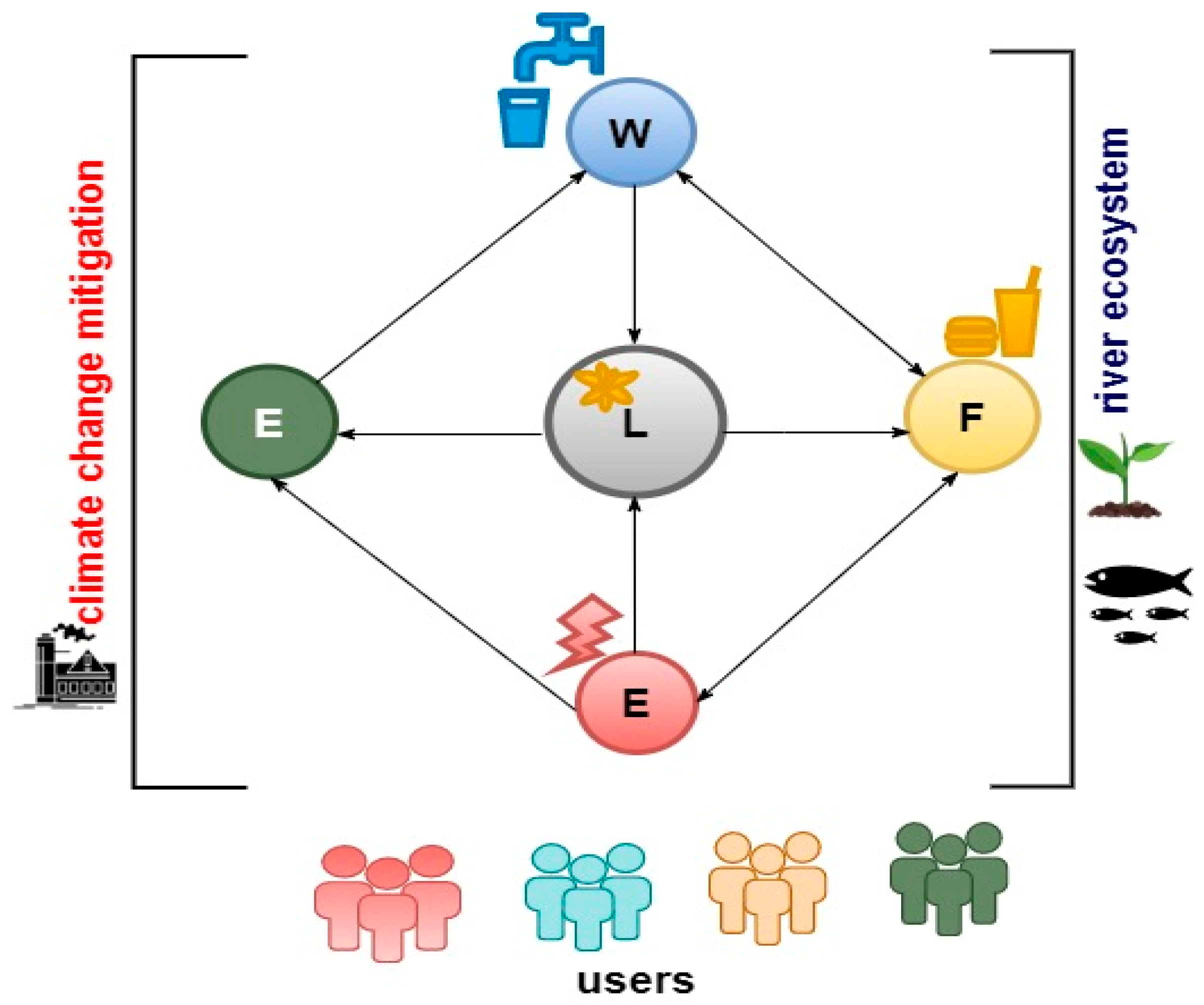
Figure 1.
Schematic representation of the land-water-food-energy-environment nexus (LWFEEN) under climate change mitigation and river ecosystem service (L—land; W—water; F—food; E—energy; E—environment).
Figure 1.
Schematic representation of the land-water-food-energy-environment nexus (LWFEEN) under climate change mitigation and river ecosystem service (L—land; W—water; F—food; E—energy; E—environment).
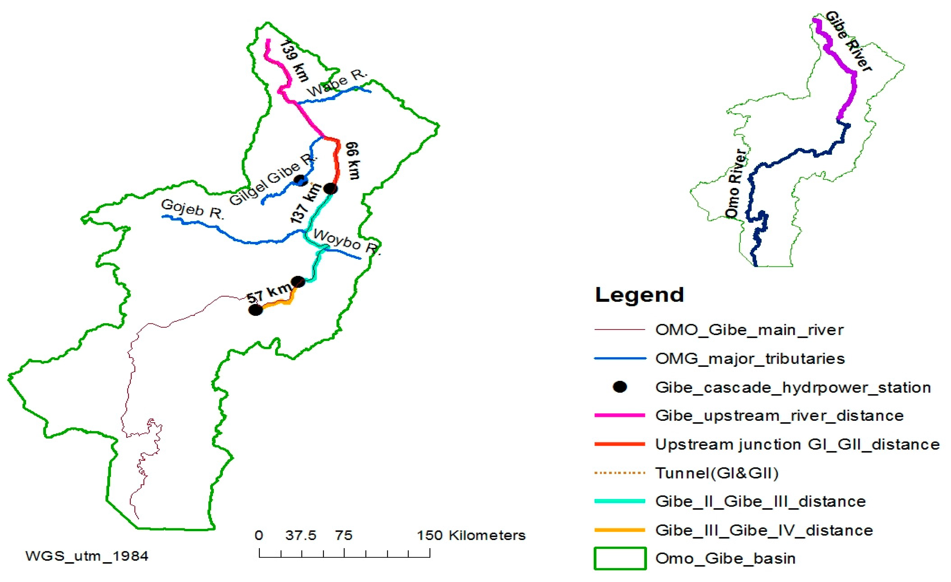
Figure 2.
Omo-Gibe River length and tributaries considered in the model.
Figure 2.
Omo-Gibe River length and tributaries considered in the model.
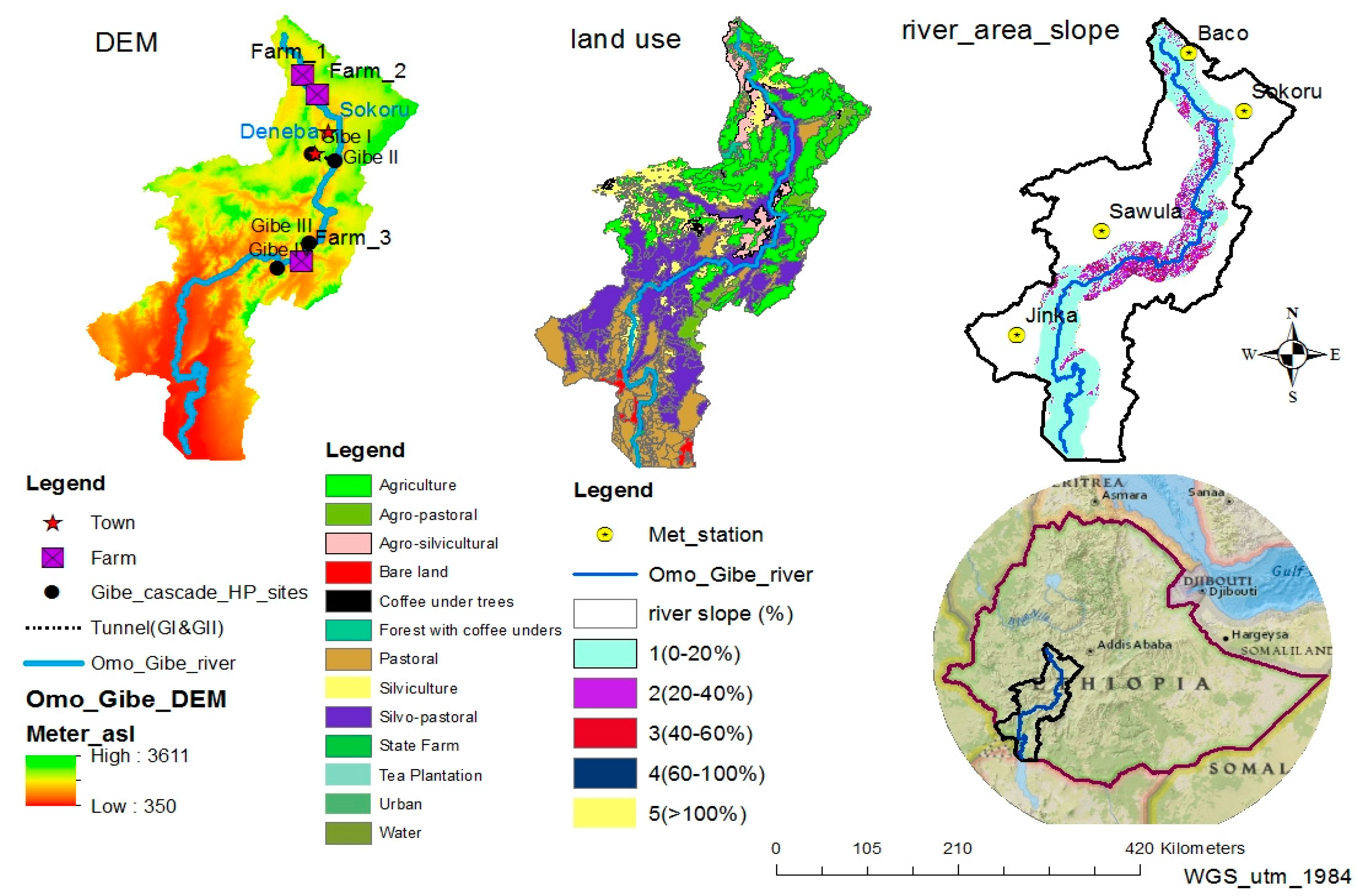
Figure 3.
Pictures of the Omo Gibe river basin showing the elevation, towns, Gibe cascade hydropower plants, land use distribution, the slope along the river length, and agricultural farms (data sources FAO, DAFNE database, 2019).
Figure 3.
Pictures of the Omo Gibe river basin showing the elevation, towns, Gibe cascade hydropower plants, land use distribution, the slope along the river length, and agricultural farms (data sources FAO, DAFNE database, 2019).
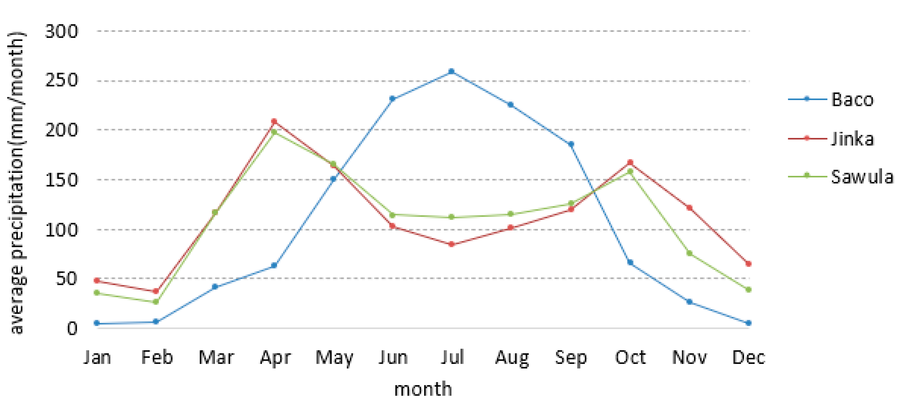
Figure 4.
Average monthly precipitation for weather stations at Baco (1998–2017), Jinka (1998–2018), and Sawula (1998–2018) [
21].
Figure 4.
Average monthly precipitation for weather stations at Baco (1998–2017), Jinka (1998–2018), and Sawula (1998–2018) [
21].
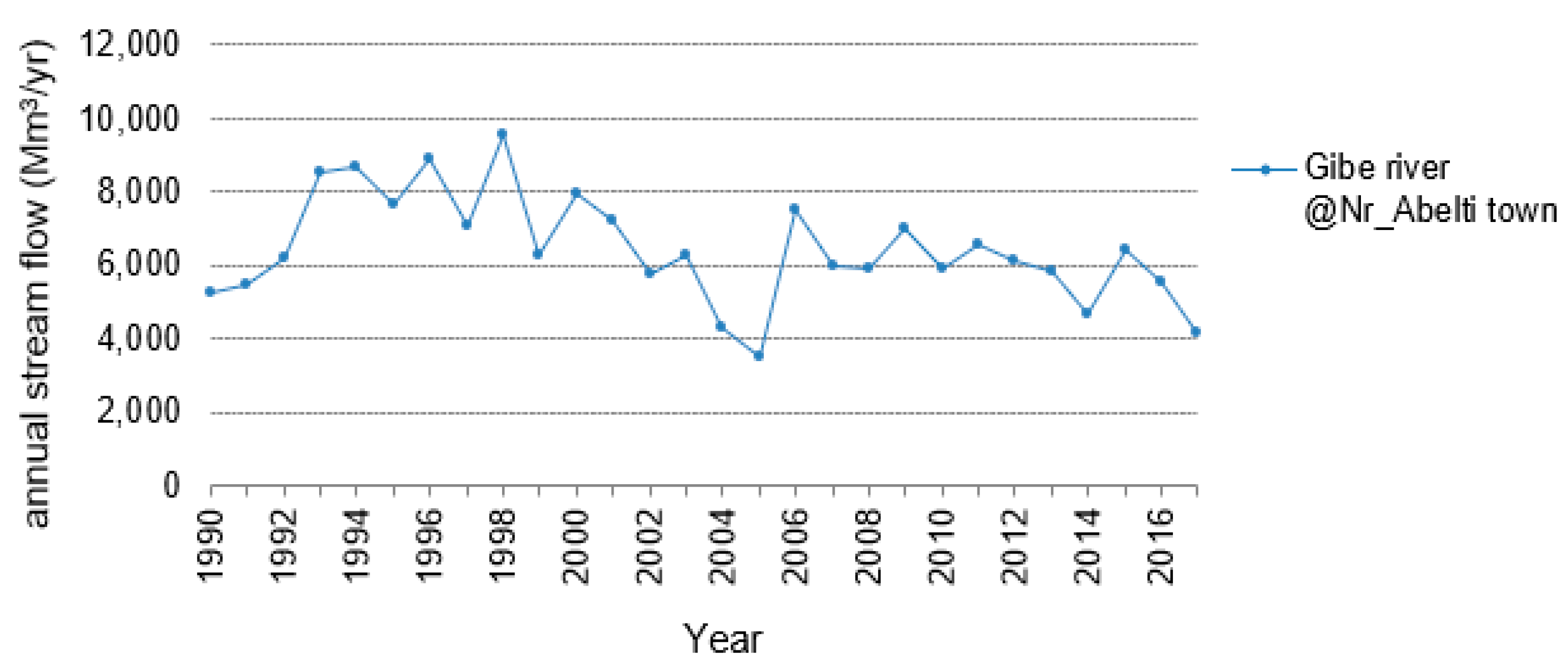
Figure 5.
Annual stream flow of Gibe river at the gauge station near the Abelti town (1990–2016) [
22].
Figure 5.
Annual stream flow of Gibe river at the gauge station near the Abelti town (1990–2016) [
22].
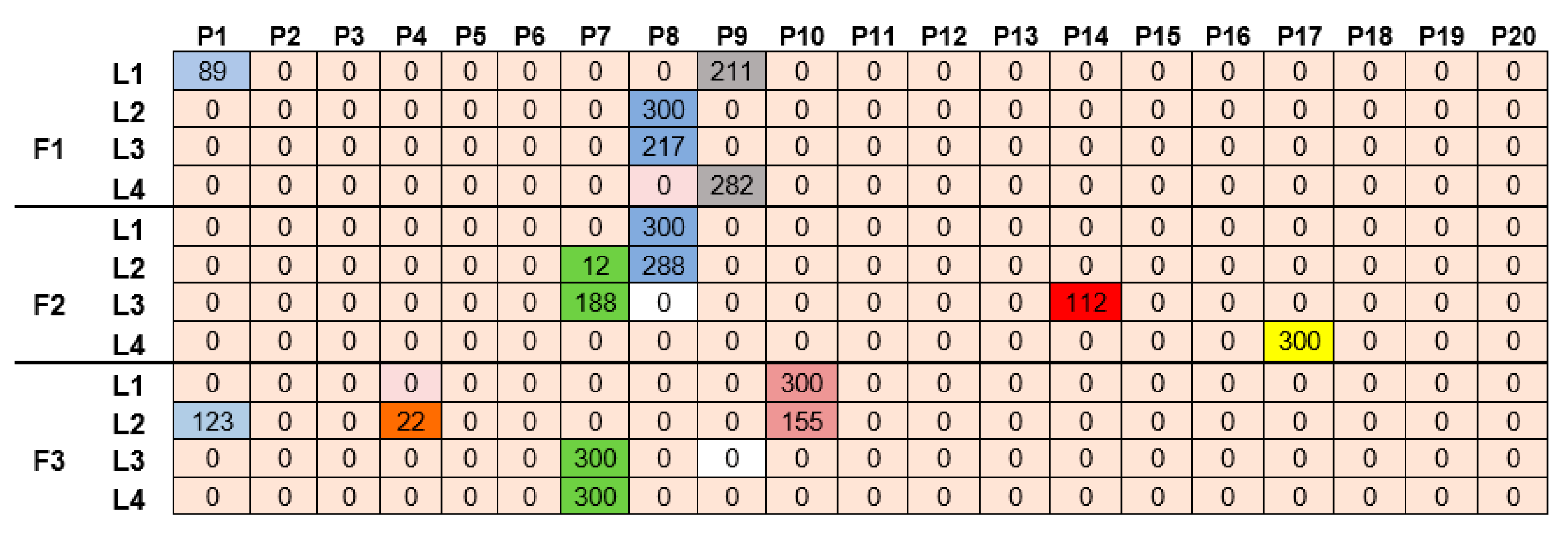
Figure 6.
Alternative crop successions format used in the model (M: maize; Bn: bean; W: wheat; F: fallow; B: barley; C: cabbage; Cr: carrot; T: teff; To: tomato; S: sorghum; Po: potato; O: onion; P: pepper), Mo: month; WK: week; L1P1: alternative crop succession to land unit 1.
Figure 6.
Alternative crop successions format used in the model (M: maize; Bn: bean; W: wheat; F: fallow; B: barley; C: cabbage; Cr: carrot; T: teff; To: tomato; S: sorghum; Po: potato; O: onion; P: pepper), Mo: month; WK: week; L1P1: alternative crop succession to land unit 1.
Figure 7.
Input data used for the land attribute data sets for alternative crop succession type P1 per unit land per week for one year. (L1P1 land unit 1 for alternative crop succession P1, food calorie(cal in MegKcal/ha/week), crop income (ci in USD/ha/week), crop production cost (cc in USD/ha/week), nitrate leaching (nl in kg/ha/week), soil loss (sl in Kg/ha/week), soil carbon sequestration (soc in Kg/ha/week). For nl, sl, and soc, here expressed in Kg but throughout the model it is used in tons.
Figure 8.
Input parameter characteristics used in the model for the alternative crop succession: (a) food calorie (cal), (b) crop income(ci), (c) crop cost (cc), (d) nitrate leaching (nl), (e) soil loss (sl), (f) soil carbon sequestration (soc), (g) crop water requirement (cwr).
Figure 8.
Input parameter characteristics used in the model for the alternative crop succession: (a) food calorie (cal), (b) crop income(ci), (c) crop cost (cc), (d) nitrate leaching (nl), (e) soil loss (sl), (f) soil carbon sequestration (soc), (g) crop water requirement (cwr).
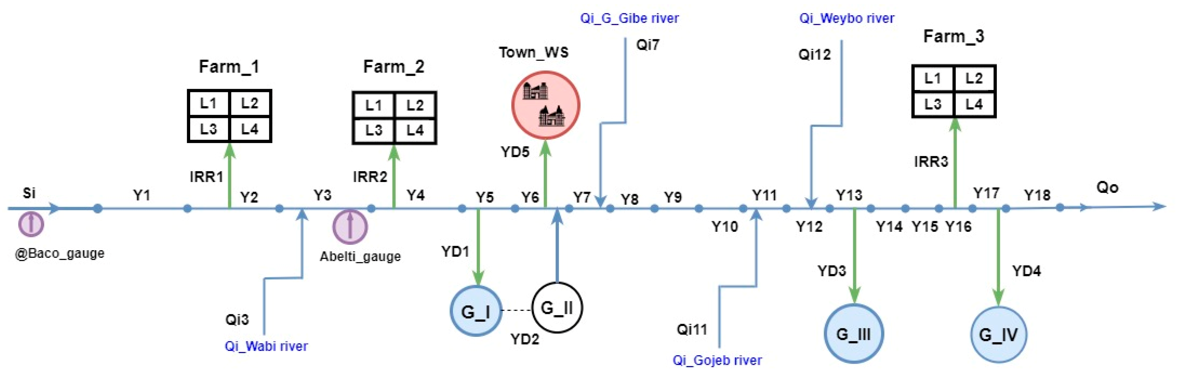
Figure 9.
Diagram of the land and river network (it has 3 farms (F1(IRR1), F2(IRR2), F3(IRR3), 4 land units (L1…L4), and 18 river segments (Y1…Y18), 4 hydropower stations/demand nodes (YD1…YD4) and 1 water supply demand node (YD5). The gauge stations are near Baco town (supply inflow) and Abelti (around the main bridge on the main road to Jimma are indicated on the diagram.
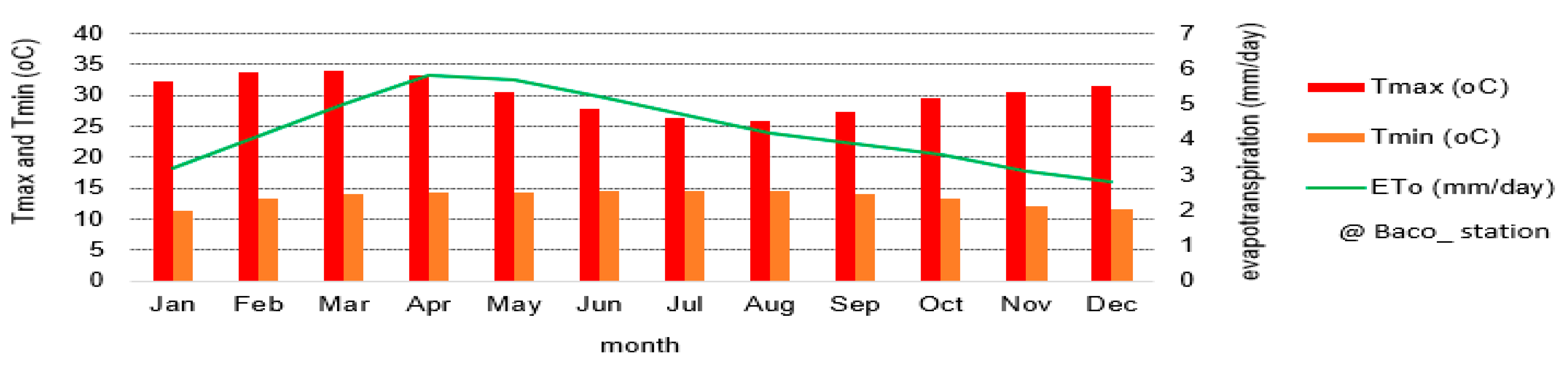
Figure 10.
Average maximum and minimum temperature and evapotranspiration at Baco weather station (1998–2017).
Figure 10.
Average maximum and minimum temperature and evapotranspiration at Baco weather station (1998–2017).
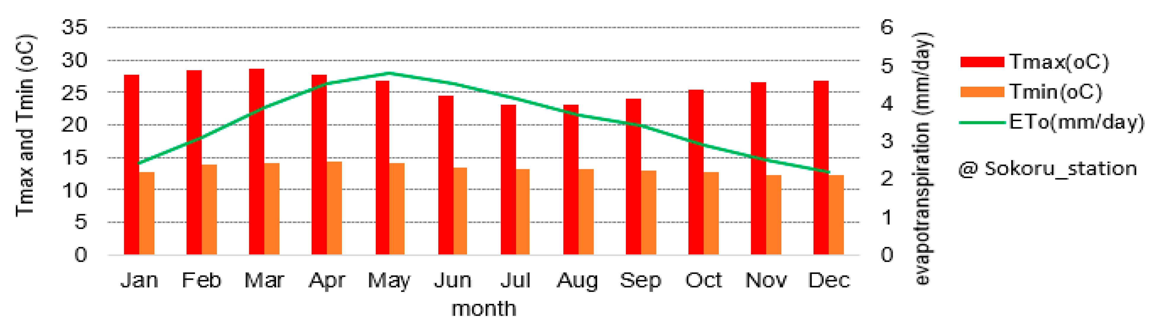
Figure 11.
Average maximum and minimum temperature and evapotranspiration at Sokoru weather station (1987–2014).
Figure 11.
Average maximum and minimum temperature and evapotranspiration at Sokoru weather station (1987–2014).
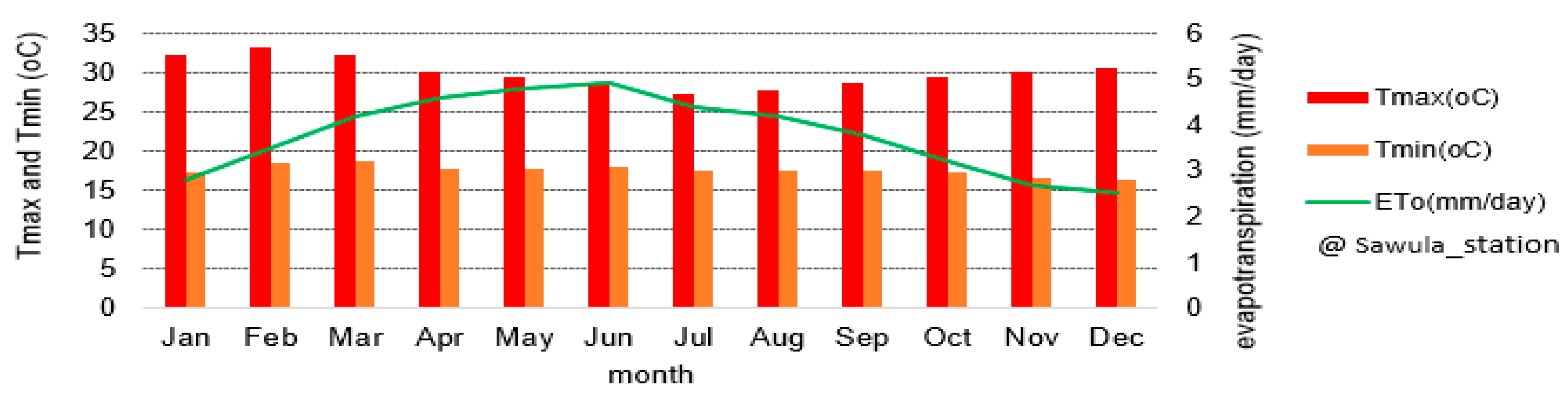
Figure 12.
Average maximum and minimum temperature and evapotranspiration at Sawula weather station (1998–2018).
Figure 12.
Average maximum and minimum temperature and evapotranspiration at Sawula weather station (1998–2018).
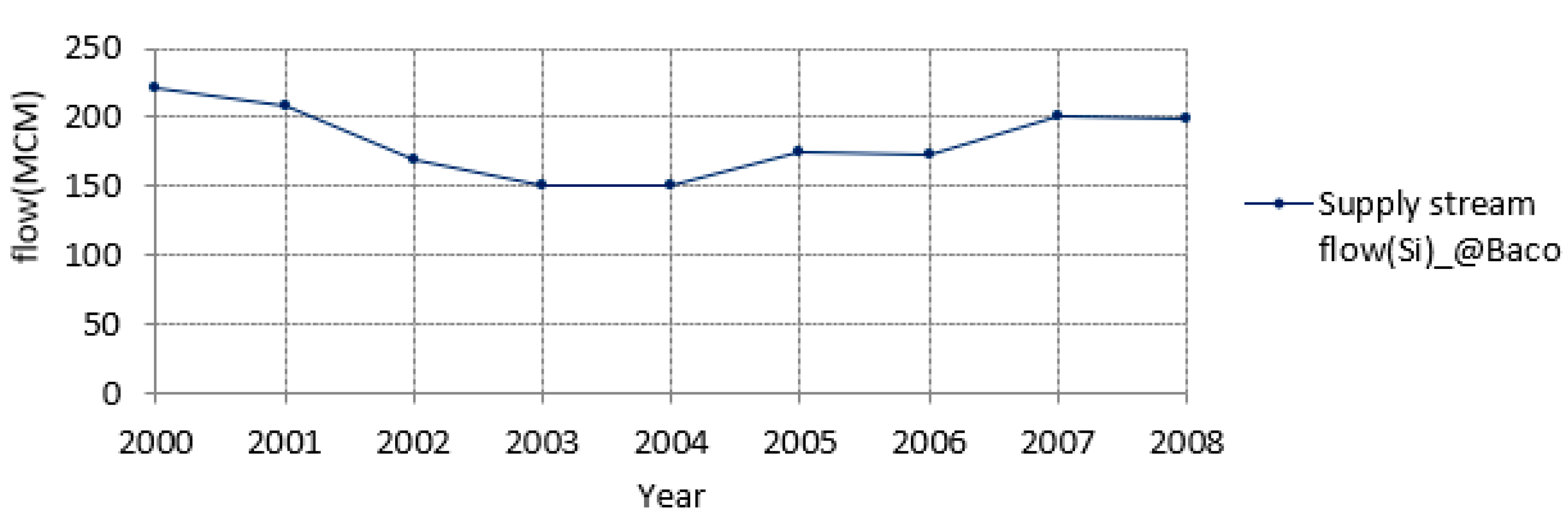
Figure 13.
Annual supply flow to Gibe river near Baco town gauging station.
Figure 13.
Annual supply flow to Gibe river near Baco town gauging station.
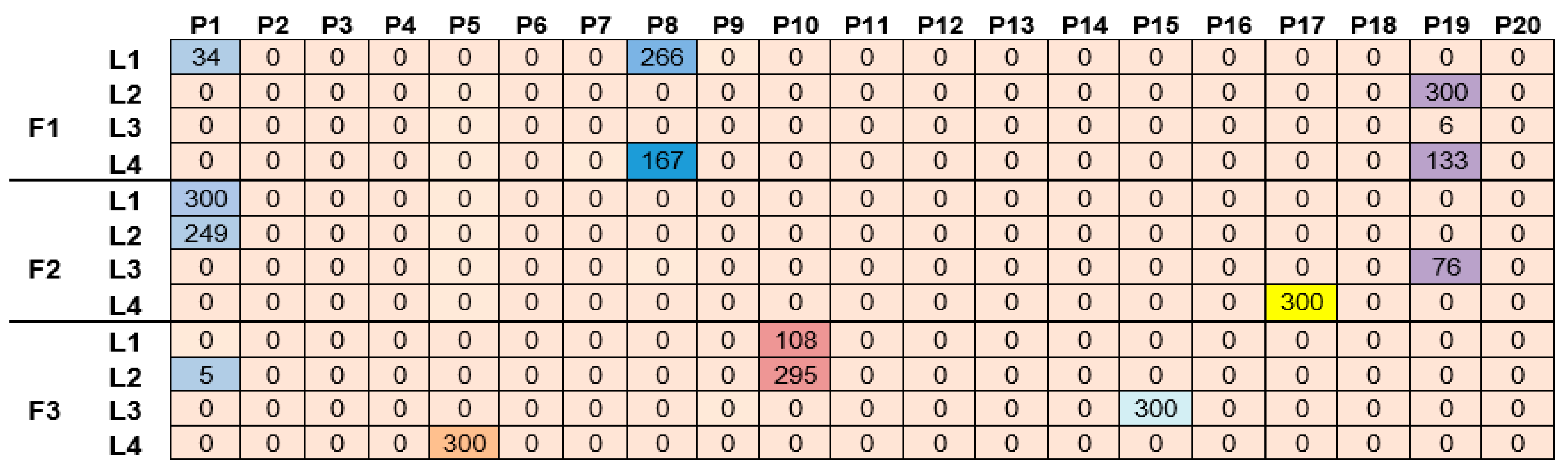
Figure 14.
Allocated alternative crop succession to land unit per farm (ha).
Figure 14.
Allocated alternative crop succession to land unit per farm (ha).
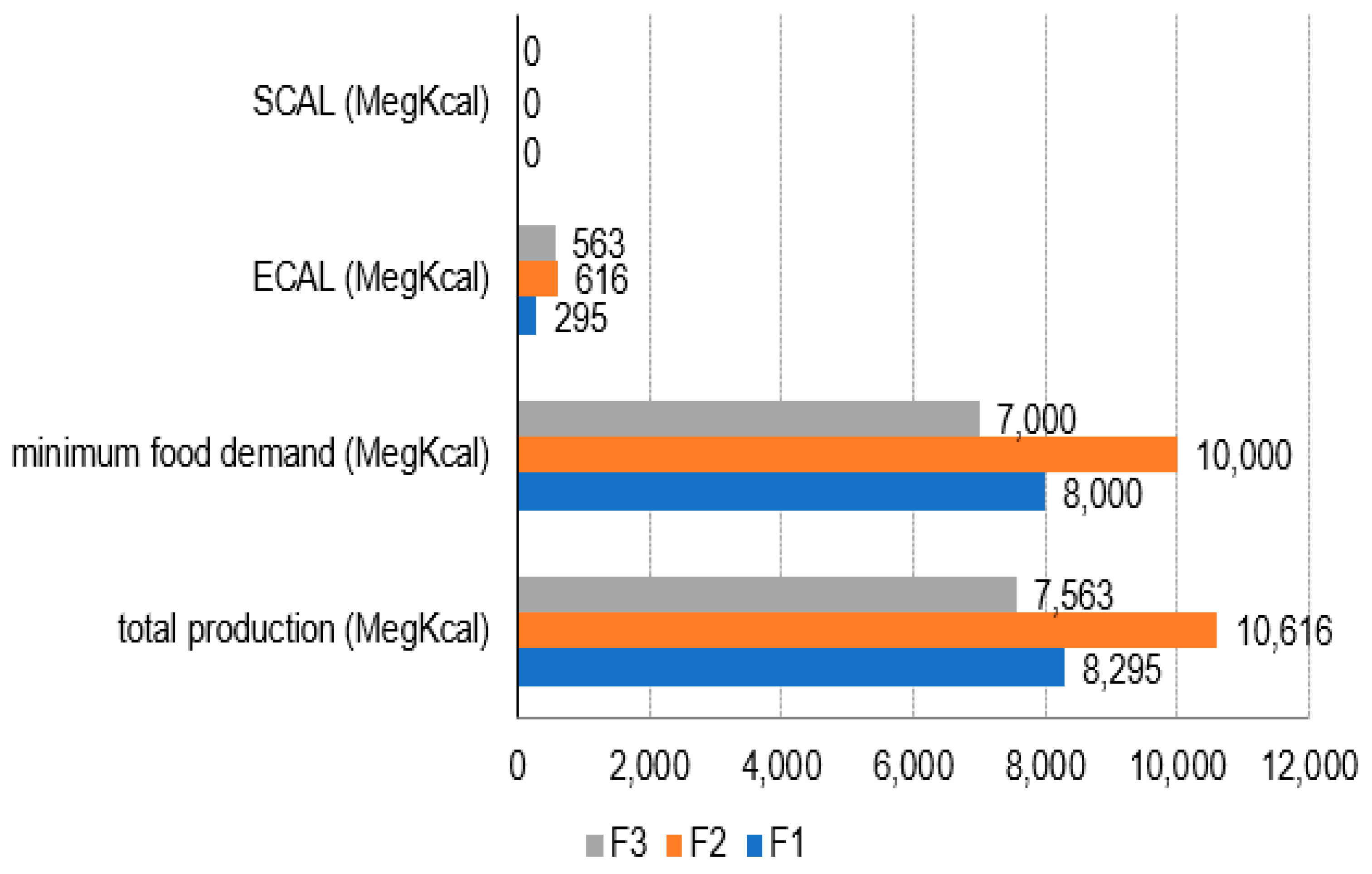
Figure 15.
Food production produced from the three farms (MegKcal/farm/year).
Figure 15.
Food production produced from the three farms (MegKcal/farm/year).
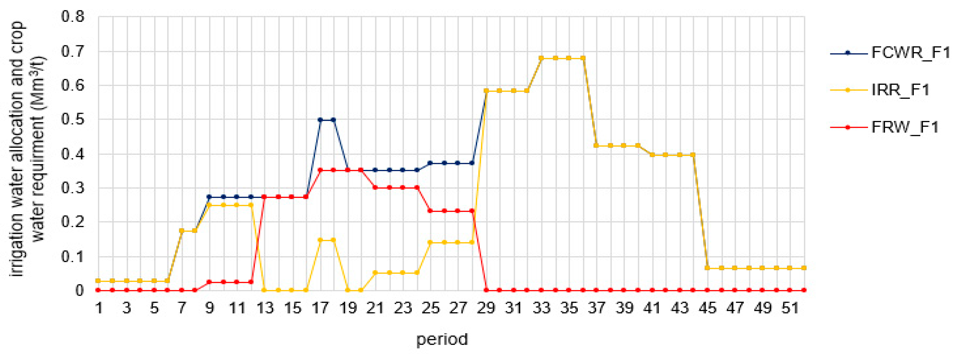
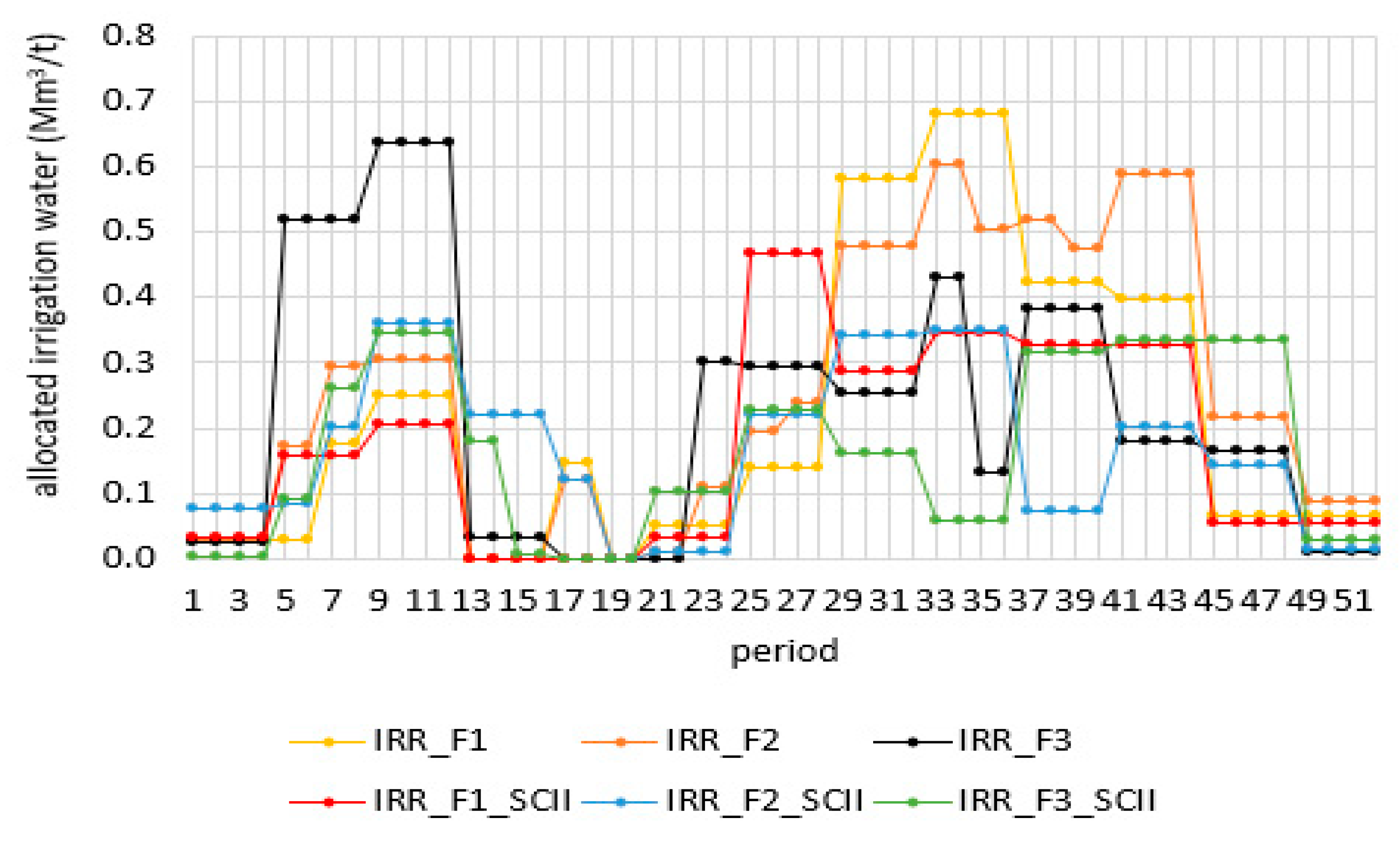
Figure 16.
Allocated irrigation water (orange), crop water requirement (blue), and available rainfall (red) for farm 1 (Omo-Gibe River basin) (Mm3/week).
Figure 16.
Allocated irrigation water (orange), crop water requirement (blue), and available rainfall (red) for farm 1 (Omo-Gibe River basin) (Mm3/week).
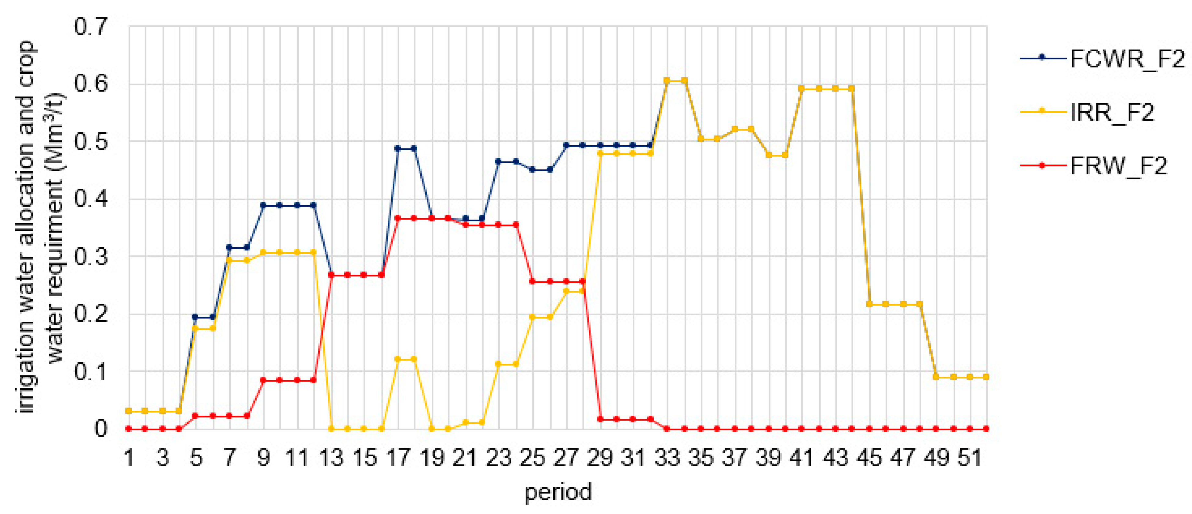
Figure 17.
Allocated irrigation water (orange), crop water requirement (blue), and available rainfall (red) for farm 2 (Omo-Gibe river basin) (Mm3/week).
Figure 17.
Allocated irrigation water (orange), crop water requirement (blue), and available rainfall (red) for farm 2 (Omo-Gibe river basin) (Mm3/week).
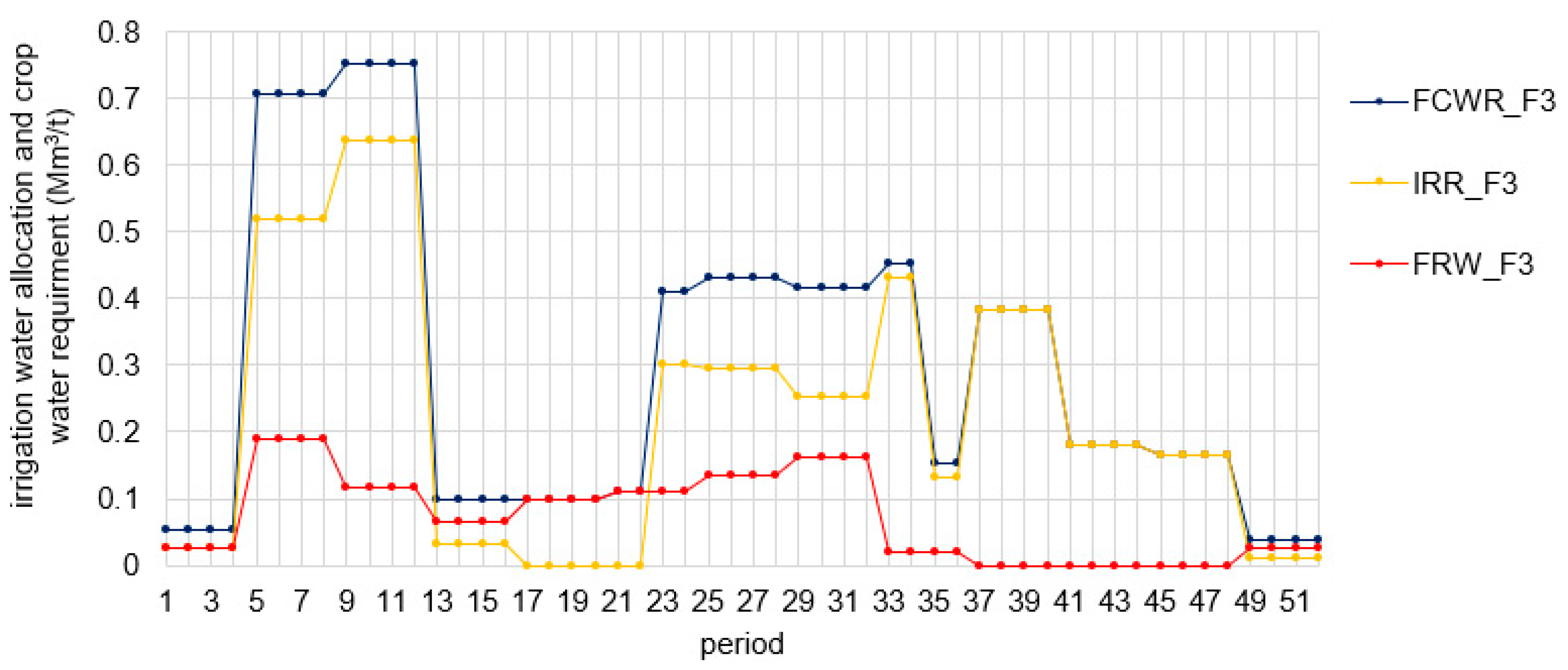
Figure 18.
Allocated irrigation water (orange), crop water requirement (blue), and available rainfall (red) for farm 3 (Omo-Gibe river basin) (Mm3/week).
Figure 18.
Allocated irrigation water (orange), crop water requirement (blue), and available rainfall (red) for farm 3 (Omo-Gibe river basin) (Mm3/week).
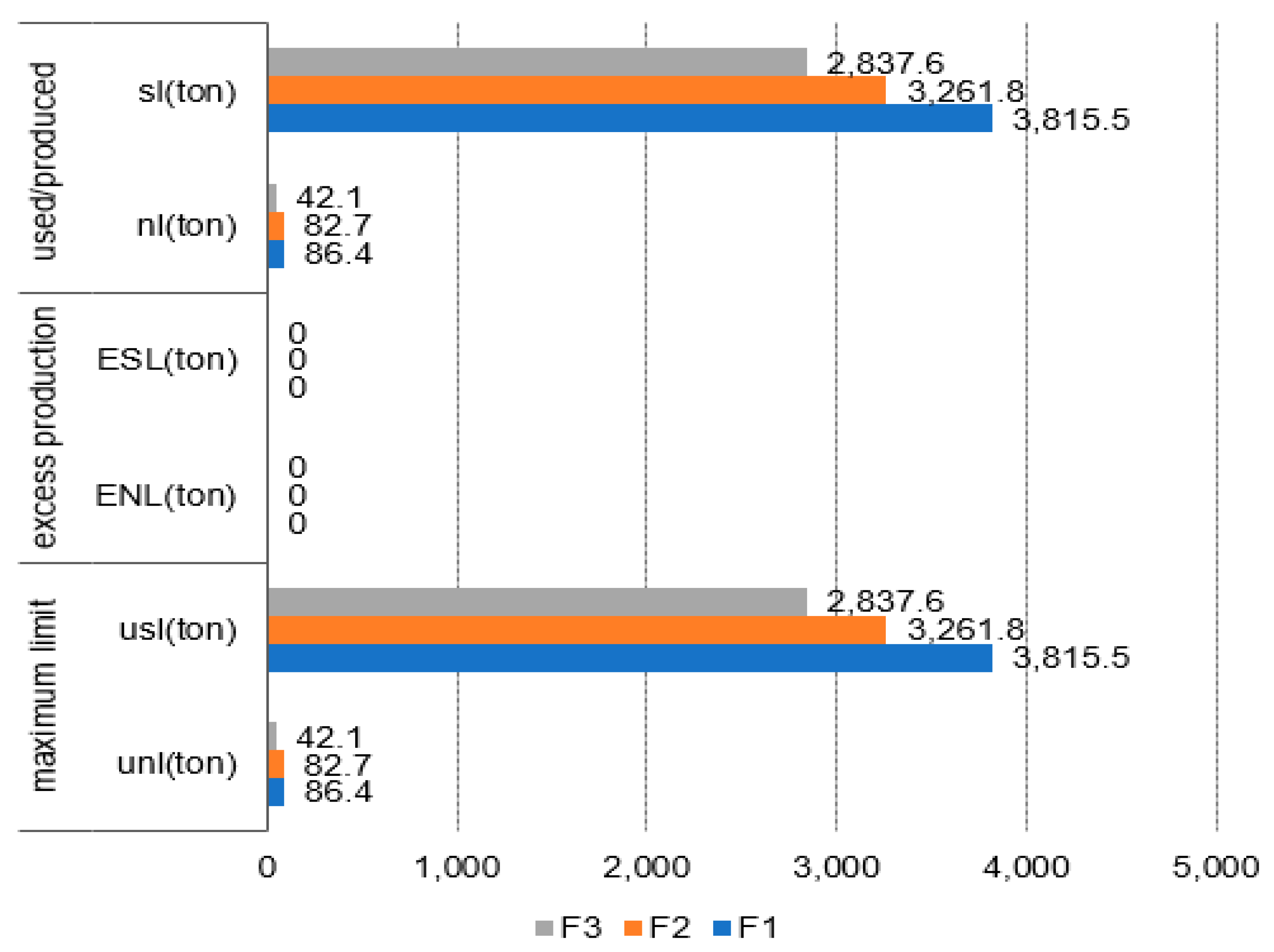
Figure 19.
Environmental induced problems from allocated alternative crop successions per farm per year(ton/farm/year) (Farm 1, 2, and 3).
Figure 19.
Environmental induced problems from allocated alternative crop successions per farm per year(ton/farm/year) (Farm 1, 2, and 3).
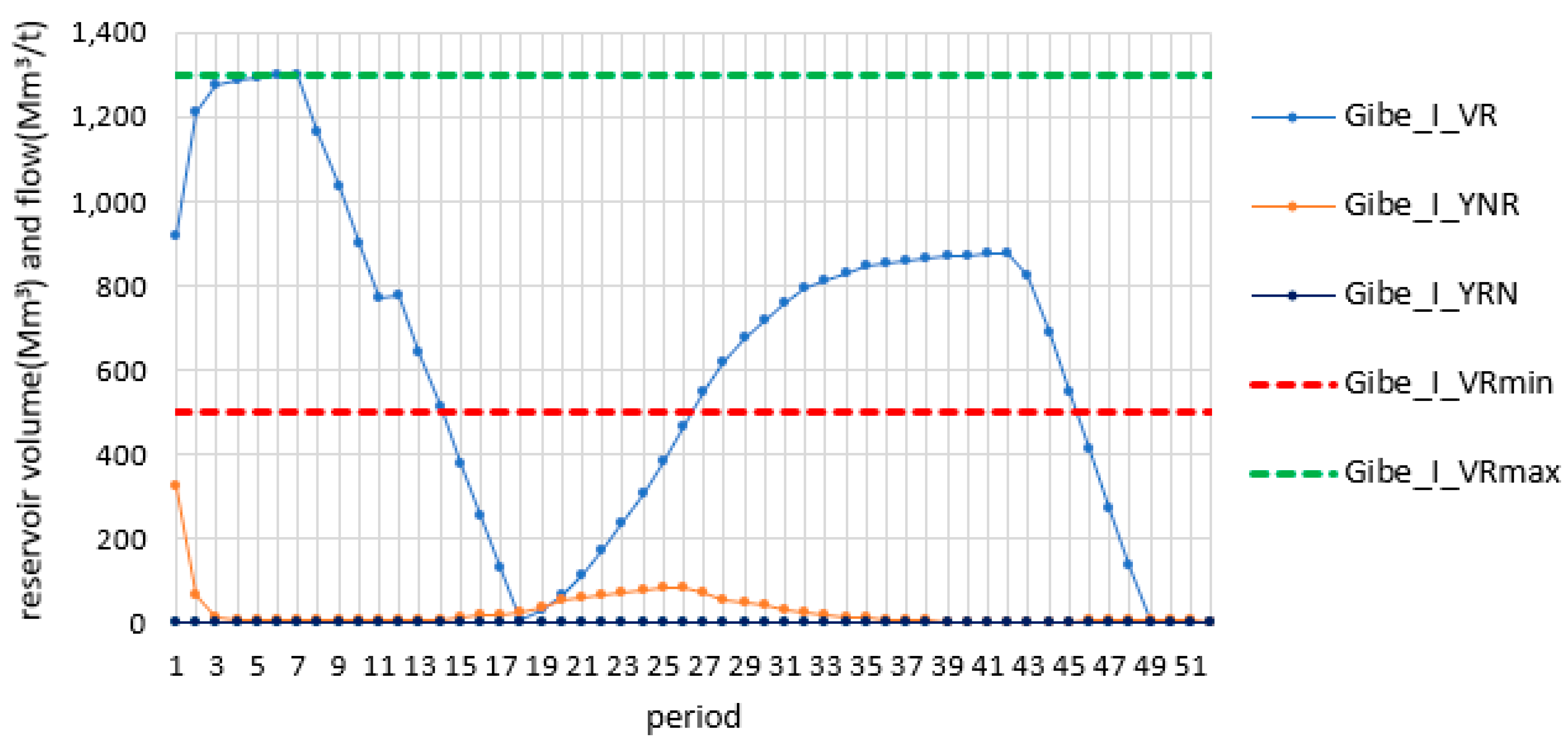
Figure 20.
Gibe_I reservoir volume storage and reservoir inflow/outflow from and to river link (Mm3:Million cubic meters).
Figure 20.
Gibe_I reservoir volume storage and reservoir inflow/outflow from and to river link (Mm3:Million cubic meters).
Figure 21.
Gibe III reservoir volume storage and inflow/outflow from and to river link.
Figure 21.
Gibe III reservoir volume storage and inflow/outflow from and to river link.
Figure 22.
Gibe IV reservoir water volume storage and inflow/outflow model simulation results.
Figure 22.
Gibe IV reservoir water volume storage and inflow/outflow model simulation results.
Figure 23.
Water allocation and unmet demand water flow for the Gibe I hydropower station (Mm3/week).
Figure 23.
Water allocation and unmet demand water flow for the Gibe I hydropower station (Mm3/week).
Figure 24.
Water allocation and unmet demand water flow for the Gibe II hydropower station (Mm3/week).
Figure 24.
Water allocation and unmet demand water flow for the Gibe II hydropower station (Mm3/week).
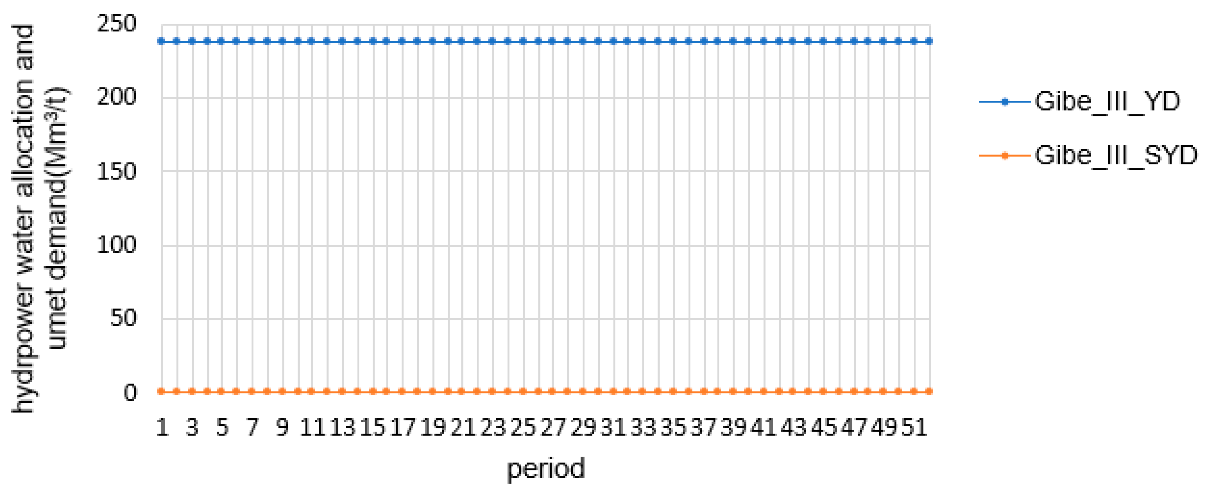
Figure 25.
Water allocation and unmet demand water flow for the Gibe III hydropower station. (Mm3/week).
Figure 25.
Water allocation and unmet demand water flow for the Gibe III hydropower station. (Mm3/week).
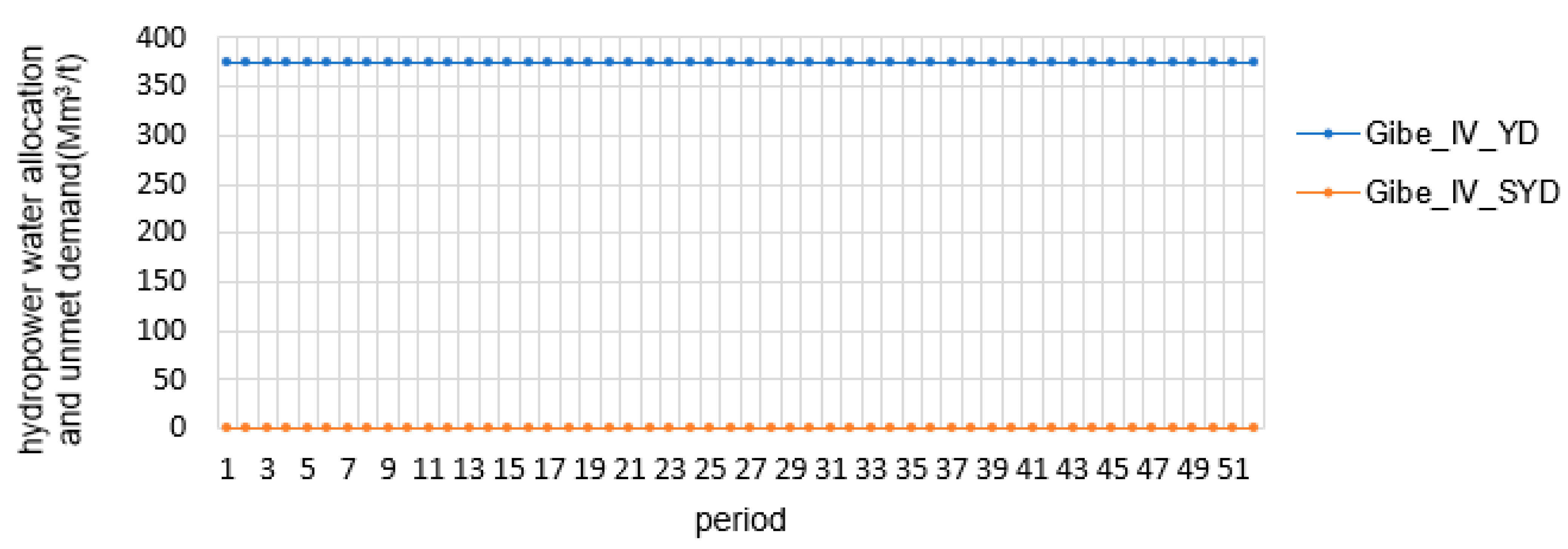
Figure 26.
Water allocation and unmet demand water flow for the Gibe IV hydropower station (Mm3/week).
Figure 26.
Water allocation and unmet demand water flow for the Gibe IV hydropower station (Mm3/week).
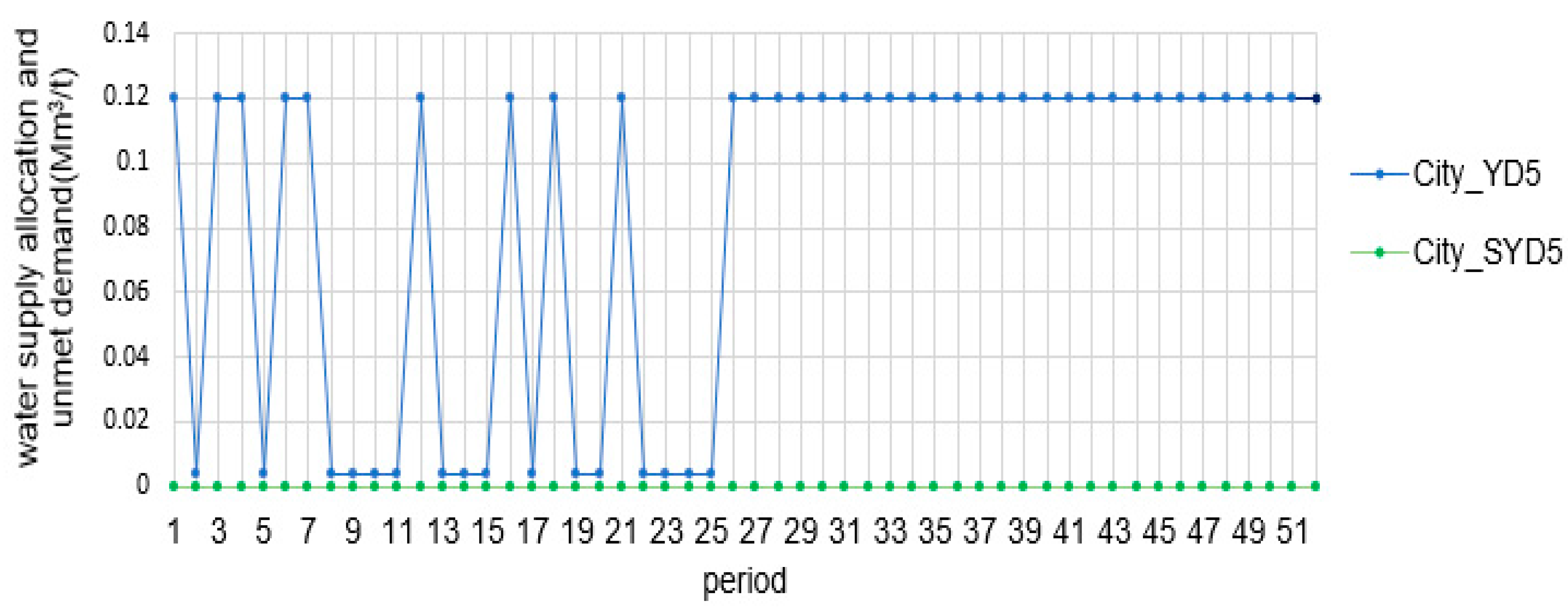
Figure 27.
Water allocation and unmet demand flow for Sokoru & Deneba towns’ municipal water supply (Mm3/week).
Figure 27.
Water allocation and unmet demand flow for Sokoru & Deneba towns’ municipal water supply (Mm3/week).
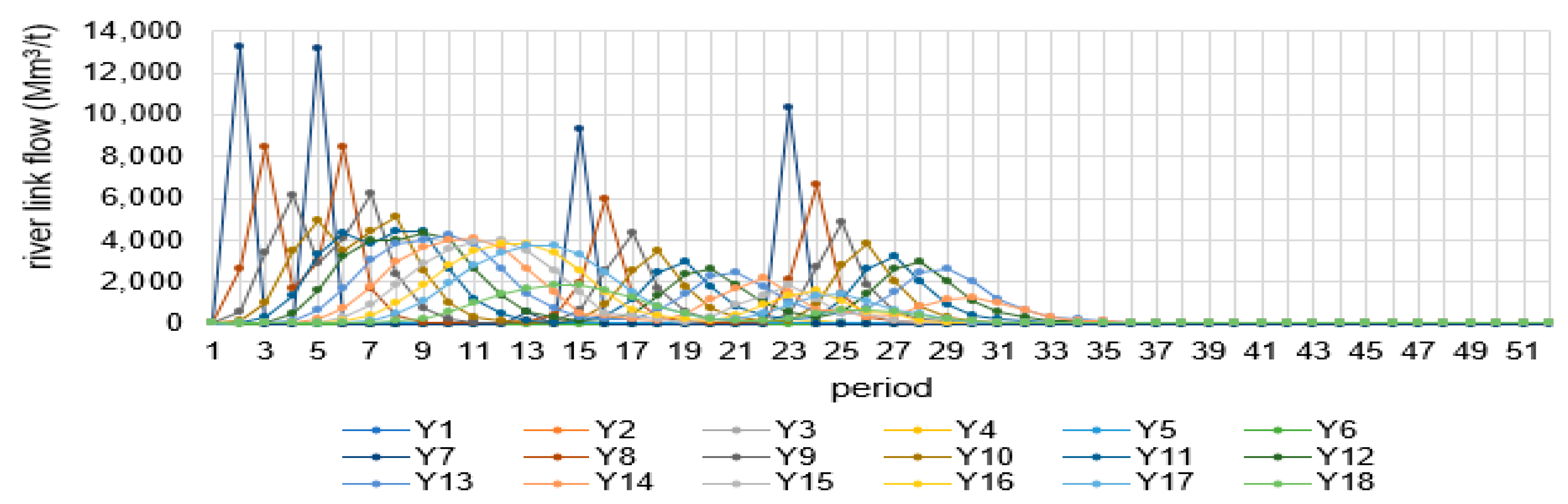
Figure 28.
Omo-Gibe river link flow model simulation results (Mm3/week).
Figure 28.
Omo-Gibe river link flow model simulation results (Mm3/week).
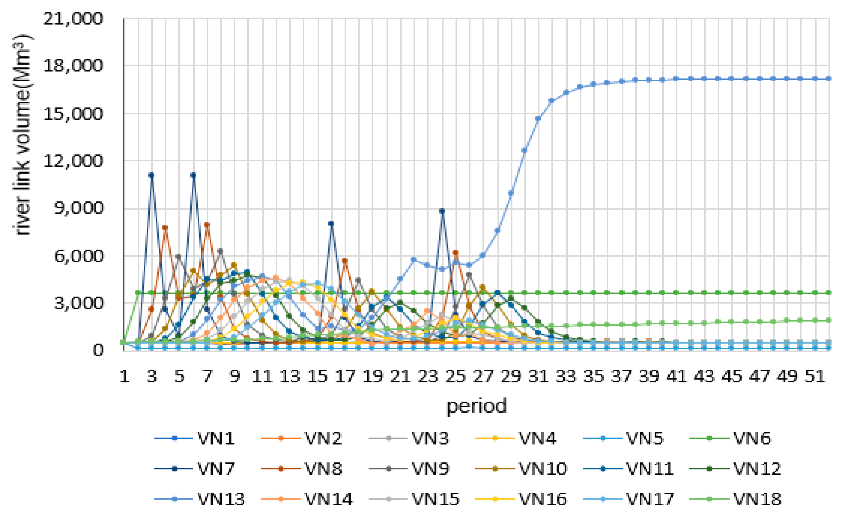
Figure 29.
Omo-Gibe river volume model simulation results.
Figure 29.
Omo-Gibe river volume model simulation results.
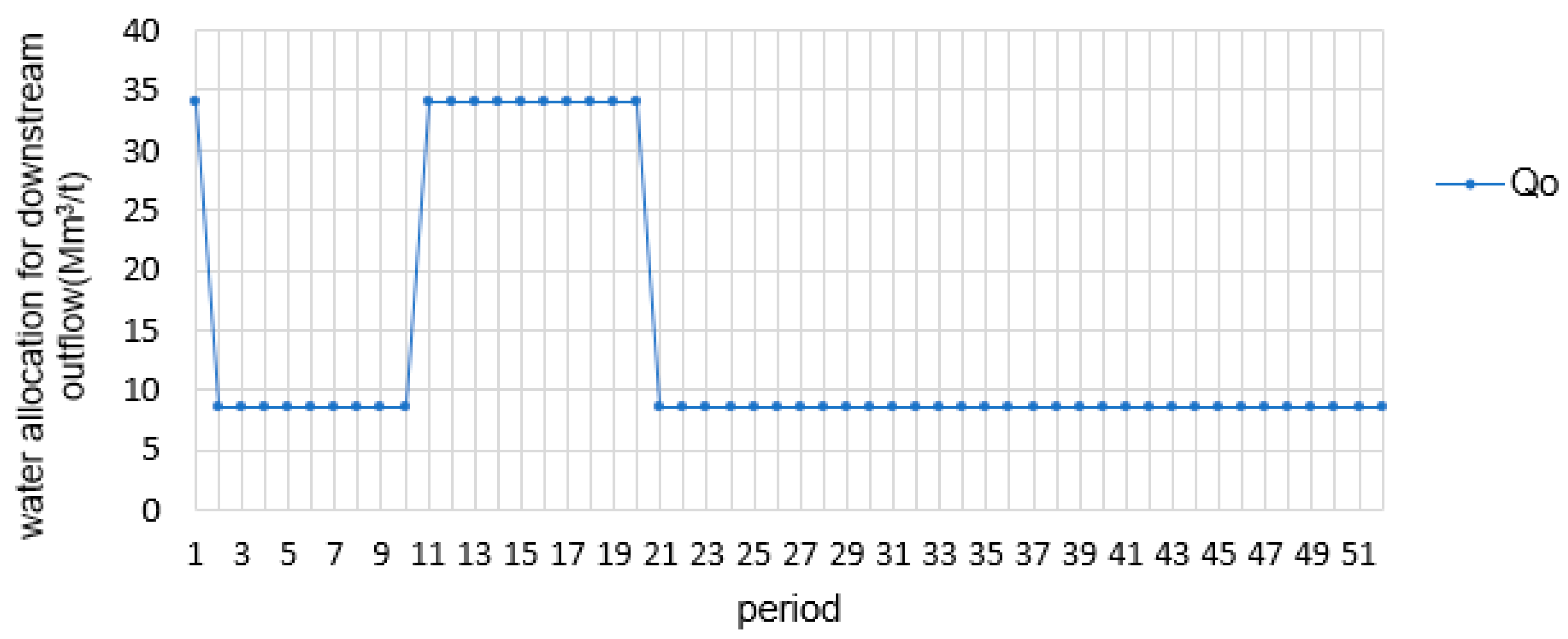
Figure 30.
Water allocation for the downstream river flow model simulation (Mm3/week).
Figure 30.
Water allocation for the downstream river flow model simulation (Mm3/week).
Figure 31.
Allocated alternative crop succession to the land unit under scenario I condition (ha).
Figure 31.
Allocated alternative crop succession to the land unit under scenario I condition (ha).
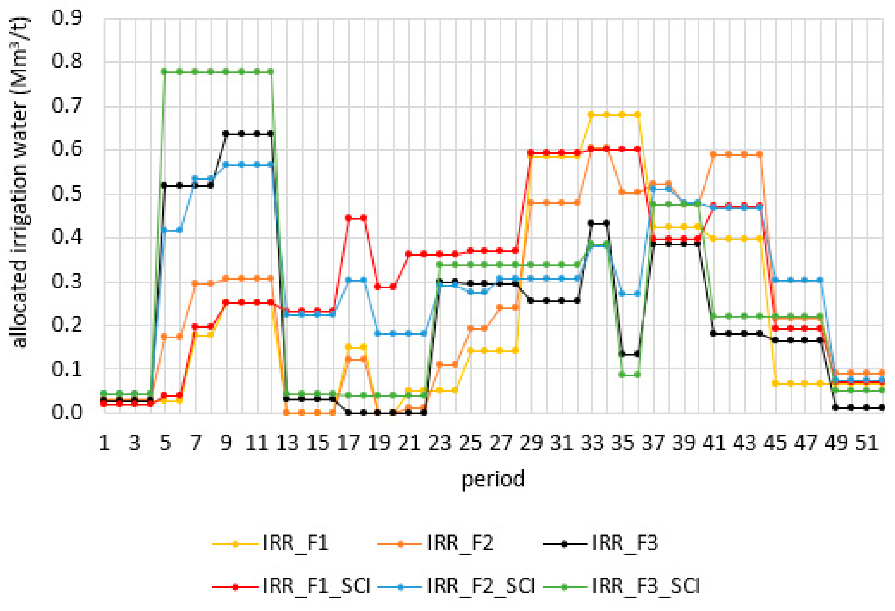
Figure 32.
Comparison of irrigation water allocation between scenario I and base scenario model conditions (Mm3/week).
Figure 32.
Comparison of irrigation water allocation between scenario I and base scenario model conditions (Mm3/week).
Figure 33.
Allocated alternative crop successions to land unit under scenario II conditions (ha).
Figure 33.
Allocated alternative crop successions to land unit under scenario II conditions (ha).
Figure 34.
Comparison of irrigation water allocation between scenario II and the initial base scenario conditions (Mm3/week).
Figure 34.
Comparison of irrigation water allocation between scenario II and the initial base scenario conditions (Mm3/week).
Table 1.
Objective and constraint function used in the model.
Table 1.
Objective and constraint function used in the model.
| Description | Equation | Unit | Eq_No. |
|---|
| Objectives | | USD | (1) |
| Constraints | | | |
| land-based constraints | | | |
| food calorie production | | MegKcal | (2) |
| minimum soil organic carbon sequestration demand | | ton | (3) |
| maximum nitrate leaching | | ton | (4) |
| maximum soil loss | | ton | (5) |
| maximum available land area size | | ha | (6) |
| minimum farm income expectation limit | | USD | (7) |
| maximum crop production budget | | ton | (8) |
| constraint(combined land and water) | | | |
| crop water requirement demand | | m3/t | (9) |
| rainfall requirement or available | | m3/t | (10) |
| irrigation water requirement | | m3 | (11) |
| water based constraint | | | |
| initial condition | | | |
| | river segment(n) | | |
| | | m3/t | (12) |
| | | m3 | (13) |
| | reservoir segment(r) | | |
| | | m3 | (14) |
| | transport(n) | | |
| | river segment(n) | | |
| river link flow continuity constraint based on the muskingum method | | m3/t | (15) |
| | | - | (16) |
| | | - | (17) |
| | | - | (18) |
| | + + =1 | - | (19) |
| flow/transport balance constraint | | | |
| | river segment | | |
| | | m3 | (20a) |
| | | m3 | (20b) |
| | reservoir link | | |
| | | m3 | (21a) |
| | | m3 | (21b) |
| | river segment | | |
| capacity constraints | | m3/t | (22) |
| | | m3/t | (23) |
| | | m3/t | (24) |
| | | m3 | (25) |
| | | m3 | (26) |
| | reservoir segment | | |
| | | m3 | (27) |
| | | m3 | (28) |
| | | m3/t | (29) |
| | demand link | | |
| | | m3/t | (30) |
| | | m3/t | (31) |
Table 2.
Indices, parameters, and variables used in the model.
Table 2.
Indices, parameters, and variables used in the model.
| Type | Notation | Description | Unit |
|---|
| indices | d | demand node d ∈ D | - |
| | f | farm f ∈ F | - |
| | j | land unit j ∈ J | - |
| | n | river link n ∈ N | - |
| | P | alternative crop succession p ∈ P | - |
| | r | reservoir link r ∈ R | - |
| | t | period t ∈ T | - |
| parameters | | | |
| | Ajf | area of land unit (j) per farm(f) | ha |
| | calpjft | food calorie per alternative crop successions (p)per land unit(j)per farm(f)per period (t) | MegKcal/ha/t |
| | ccpjft | crop production cost of alternative crop successions (p) per land unit(j)per farm(f)per period (t) | USD/ha/t |
| | cipjft | crop income per alternative crop successions (p)per land unit(j)per farm(f)per period (t) | USD/ha/t |
| | C0, C1, C2 | routing coefficient | - |
| | cwrpjft | crop water requirement per alternative crop successions (p) per land unit(j)per farm(f)per period (t) | m3/ha/t |
| | Dmindt | demand volume water needed at node d per period(t) | m3/t |
| | Dmaxdt | maximum demand volume water needed at node d per period(t) | m3/t |
| | Lcalf | minimum calorie requirement per farm,∀(f) ∈f | USD |
| | Lcif | minimum crop income requirement per farm,∀(f) ∈f | USD |
| | Lsocf | minimum soil organic carbon sequestration demand per farm(f), ∀(f) ∈f | ton |
| | nlpjft | nitrate leaching of alternative crop successions (p) per land unit(j)per farm(f)per period (t) | ton/ha/t |
| | Pcal | penalty for unmet food calorie production at farm | USD/MegKcal |
| | Pd | penalty for unmet demand at demand link d | USD/m3 |
| | Pr | cost for water travel to and from reservoir to river link r. | USD/m3 |
| | pvr | penalty for unmet reservoir volume of minimum requirement at reservoir r | USD/m3 |
| | Qomaxnt | maximum outflow at downstream end river link(n) | m3/t |
| | Qominnt | minimum outflow demand at downstream river link(n) | m3/t |
| | Sin,t | upstream inflow at the start of river link(n) per period(t) | m3/t |
| | Resmaxoutflowrt | reservoir outflow maximum limit t; ∀(r) ∈ r | m3/t |
| | rwft | rainwater per crop pattern (p) per farm(f) per period(t) | m3/ha/t |
| | slpjft | soil loss of alternative crop successions (p) per land unit(j)per farm(f)per period (t) | ton/ha/t |
| | socpjft | soil organic carbon sequestration of alternative crop successions (p) per land unit(j)per farm(f)per period (t) | ton/ha/t |
| | Uccf | maximum crop production budget allowed per farm,∀(f) ∈f | USD |
| | unlf | maximum nitrate leaching demand per farm(f),∀(f) ∈f | ton |
| | uslf | maximum soil loss demand per farm(f), ∀(f) ∈f | ton |
| | VNmaxn | maximum water volume needed on river link (n), ∀(n) ∈ n | m3 |
| | VNminn | minimum water volume needed on river link (n), ∀(n) ∈ n | m3 |
| | VNt=0 | initial water volume on river link n, ∀(n) ∈ n | m3 |
| | VRinitialrt=0 | initial reservoir volume on reservoir r,∀(r) ∈r | m3 |
| | VRmaxr | maximum reservoir volume on reservoir link r, ∀(r) ∈r | m3 |
| | VRminr | minimum of reservoir volume limit, ∀(r) ∈r | m3 |
| | w | the Muskingum weighting factor of river link (n,); ∀(n) ∈ n | - |
| | Yminn | minimum water flow needed on river link (n), ∀(n) ∈ n | m3/t |
| | Ynt=0 | initial water inflow on river link n, ∀(n) ∈ n | m3/t |
| variables | | | |
| | ECALf | excess calorie production per farm f, ∀(f) ∈f | MegKcal |
| | ENLf | excess nitrate leaching per farm f, ∀(f) ∈f | ton |
| | ESLf | excess soil loss per farm f, ∀(f) ∈f | ton |
| | FCWRft | total crop water requirement for allocated crop per farm per time t; ∀(f) ∈f | m3/t |
| | FRWft | total rainwater available for allocated alternative crop successions per farm per time t; ∀(f) ∈f | m3/t |
| | IRRft | irrigation water allocated for allocated alternative crop successions per farm f per period time t; ∀(f) ∈f | m3/t |
| | Qont | downstream river link end outflow at river link n at time t; ∀(n) ∈ n | m3/t |
| | SCALf | unmet food calorie production per farm f, ∀(f) ∈f | MegKcal |
| | SSOCf | unmet soil organic carbon sequestration per farm | ton |
| | SYDdt | unmet demand at demand link d at time t | m3/t |
| | SVRr | unmet reservoir minimum volume capacity limit of reservoir r, ∀(r) ∈r | m3 |
| | VN,n | water volume on river link n at beginning of time t; ∀(n) ∈ n | m3 |
| | VRr | reservoir volume r, ∀(r) ∈r | m3 |
| | Xpjf | allocated cropland per alternative crop successions p,per land unit j,per farm f, ∀(p) ∈p, ∀(j) ∈ j, ∀(f) ∈ f | ha |
| | YDdt | water allocation on-demand link or demand node d at time t;
∀(d) ∈ d | m3/t |
| | YNRrt | reservoir inflow from river link to reservoir link r, at time t ∀(r) ∈ r | m3/t |
| | Ynt | water flow on river link n at time t ∀(n) ∈ n | m3/t |
| | YRNrt | reservoir outflow from river link to reservoir link r, at time t ∀(r) ∈ r | m3/t |
Table 3.
Average precipitation in the Omo_Gibe river basin (mm/month).
Table 3.
Average precipitation in the Omo_Gibe river basin (mm/month).
| Year | | Jan | Feb | Mar | Apr | May | Jun | Jul | Aug | Sep | Oct | Nov | Dec |
|---|
| 1998_2017 | Baco | 4.7 | 5.8 | 42.0 | 63.6 | 150.7 | 231.5 | 258.3 | 225.3 | 184.6 | 66.1 | 26.5 | 4.4 |
| average eff.p | farm1 | 0 | 0 | 0 | 0 | 9.3 | 106.7 | 141.8 | 121.2 | 91.0 | 0 | 0 | 0 |
| 1987_2014 | Sokoru | 32.7 | 33.6 | 79.0 | 115.9 | 149.7 | 203.1 | 237.1 | 222.1 | 172.7 | 77.2 | 25.8 | 22.4 |
| average eff.p | farm2 | 0 | 0 | 0 | 7.9 | 30.7 | 95.1 | 135.4 | 130.3 | 91.1 | 5.3 | 0 | 0 |
| 1998_2018 | Sawula | 35.4 | 26.9 | 116.6 | 197.5 | 165.5 | 114.1 | 111.7 | 115.2 | 125.4 | 157.7 | 74.7 | 38.6 |
| average eff.p | farm3 | 0 | 0 | 12.4 | 87.1 | 46.5 | 0 | 2.6 | 11 | 34.2 | 78.3 | 9.9 | 0 |
Table 4.
Average monthly river inflow (Mm3/month).
Table 4.
Average monthly river inflow (Mm3/month).
| Year | St | Area | Jan | Feb | Mar | Apr | May | Jun | Jul | Aug | Sep | Oct | Nov | Dec |
|---|
| 2000–2008 | Supply_Nr_Baco | - | 11.7 | 6.7 | 6.9 | 4.9 | 7.0 | 14.7 | 22.4 | 34.8 | 30.6 | 18.4 | 12.1 | 13.0 |
| 2000_2019 | Gibe_Nr_Asendabo | 2966 sq Km | 22.8 | 16.2 | 18.3 | 26.3 | 67.6 | 113.4 | 241.5 | 310.1 | 284.1 | 123.4 | 58.6 | 31.9 |
| 2000_2017 | Gojeb_nr_Shebe | 3577.0 sq km | 32.5 | 18.9 | 26.1 | 52.4 | 118.2 | 182.6 | 321.8 | 379.2 | 396.6 | 268.9 | 138.1 | 65.6 |
| 1992_2006 | Weybo_nr_Areka | 2368.4 sq km | 0.9 | 0.6 | 1.0 | 2.0 | 3.9 | 3.0 | 7.5 | 12.8 | 7.6 | 9.7 | 5.0 | 2.6 |
| 2000_2007 | Wabi_nr_Welkite | 1866.0 sq km | 9.9 | 11.2 | 16.7 | 36.4 | 32.3 | 78.8 | 255.0 | 340.8 | 150.2 | 46.4 | 13.2 | 8.3 |
| 1990_2017 | Gibe_Nr_Abelti | 15746 sq Km | 69.2 | 94.1 | 94.4 | 108.3 | 120.1 | 328.4 | 1013.7 | 1784.0 | 1360.6 | 935.7 | 341.4 | 190.2 |
Table 5.
Input data used for land-based constraints.
Table 5.
Input data used for land-based constraints.
| Type | (MegKcal/Year) | Lci (USD/Year) | ucc (USD/Year) | Lsoc (ton/Year) | unl (ton/Year) | usl (ton/Year) | A (ha) | Total Farm Size (ha) | Land-Based Penalty |
|---|
| Farm1 | 8000 | 1,500,000 | 462,988.8 | 465.3 | 86.4 | 3815.5 | 300 | 1200 | penalty for unmet food calorie production(USD/MegKcal/year)_Pcal | 9 |
| Farm2 | 10,000 | 1,500,000 | 483,776.9 | 491.7 | 82.7 | 3261.8 | 300 | 1200 | penalty for unmet soil organic carbon sequestration (USD/ton/year)_Pssoc | 5 |
| Farm3 | 7000 | 1,500,000 | 388,814.7 | 449.5 | 42 | 2837.6 | 300 | 1200 | penalty for excess nitrate leaching(USD/ton/year)_Penl | 6 |
| | | | | | | | | | penalty for excess soil loss(USD/ton/year)_Pesl | 8 |
Table 6.
Input data used in the model for river link part constraints.
Table 6.
Input data used in the model for river link part constraints.
| Link | Node | | | Routing Coefficient | River Link Flow (Mm3) | River Link Volume Capacity (Mm3) | Minimum/Maximum River End Outflow (Mm3) |
|---|
| River Link (n) | from | to | k | w | C0 | CONE | CTWO | Ymin | Yinitial | VNmin | VNmax | VNinitial | Qomin | Qomax |
|---|
| 1 | 1 | 2 | 1 | 0.25 | 0.2 | 0.6 | 0.2 | 0.5 | 0 | 95 | 1100 | 500 | - | - |
| 2 | 2 | 3 | 1 | 0.25 | 0.2 | 0.6 | 0.2 | 1 | 1.8 | 100 | 1200 | 500 | - | - |
| 3 | 3 | 4 | 1 | 0.25 | 0.2 | 0.6 | 0.2 | 1 | 1.8 | 100 | 1200 | 500 | - | - |
| 4 | 4 | 5 | 1 | 0.25 | 0.2 | 0.6 | 0.2 | 1 | 1.8 | 100 | 1200 | 500 | - | - |
| 5 | 5 | 6 | 1 | 0.25 | 0.2 | 0.6 | 0.2 | 1 | 1.8 | 100 | 1200 | 500 | - | - |
| 6 | 6 | 7 | 1 | 0.25 | 0.2 | 0.6 | 0.2 | 1 | 2.5 | 100 | 3629.9 | 500 | - | - |
| 7 | 7 | 8 | 1 | 0.25 | 0.2 | 0.6 | 0.2 | 1 | 2.5 | 100 | 11,094.2 | 500 | - | - |
| 8 | 8 | 9 | 1 | 0.25 | 0.2 | 0.6 | 0.2 | 1.1 | 3 | 100 | 8378.13 | 500 | - | - |
| 9 | 9 | 10 | 1 | 0.25 | 0.2 | 0.6 | 0.2 | 1.2 | 3 | 100 | 8178.5 | 500 | - | - |
| 10 | 10 | 11 | 1 | 0.25 | 0.2 | 0.6 | 0.2 | 1.2 | 3 | 100 | 7282.5 | 500 | - | - |
| 11 | 11 | 12 | 1 | 0.25 | 0.2 | 0.6 | 0.2 | 2 | 4 | 100 | 6622.7 | 500 | - | - |
| 12 | 12 | 13 | 1 | 0.25 | 0.2 | 0.6 | 0.2 | 2 | 4 | 150 | 6100 | 500 | - | - |
| 13 | 13 | 14 | 1 | 0.25 | 0.2 | 0.6 | 0.2 | 2 | 4 | 160 | 17,961.9 | 500 | - | - |
| 14 | 14 | 15 | 1 | 0.25 | 0.2 | 0.6 | 0.2 | 2 | 4.5 | 160 | 6600 | 500 | - | - |
| 15 | 15 | 16 | 1 | 0.25 | 0.2 | 0.6 | 0.2 | 2 | 4.5 | 160 | 6600 | 500 | - | - |
| 16 | 16 | 17 | 1 | 0.25 | 0.2 | 0.6 | 0.2 | 2 | 4.5 | 150 | 5684.1 | 500 | - | - |
| 17 | 17 | 18 | 1 | 0.25 | 0.2 | 0.6 | 0.2 | 2 | 3 | 150 | 5200.6 | 500 | - | - |
| 18 | 18 | 19 | 1 | 0.25 | 0.2 | 0.6 | 0.2 | 2 | 3 | 120 | 5100 | 500 | - | - |
| 19 | 19 | - | | | | | | | | | | | 8.5 | 34 |
Table 7.
Input data used in the model for reservoir link part constraints.
Table 7.
Input data used in the model for reservoir link part constraints.
| Res_Link (n) | Volume (Mm3) | Flow (Mm3/Week) | Cost for Water Travel between Reservoir-River Link (USD/Mm3/Week) | Penalty for Unmet Reservoir Storage (USD/Mm3/Week) |
|---|
| | VRinitial | VRmin | VRmax | Resmaxoutflow | pr | Pvr |
| 1 | 917 | 500 | 1300 | 1000 | 0.0003 | 0.5 |
| 2 | 11,750 | 8000 | 16,000 | 1500 | 0.0003 | 0.5 |
| 3 | 10,000 | 7000 | 16,000 | 2000 | 0.003 | 0.5 |
Table 8.
Input data for the demand node link.
Table 8.
Input data for the demand node link.
| Demand Type | Demand Node | Minimum Demand Capacity Limit (mm3) | Penalty (USD/Mm3/Week) |
|---|
| | d | Dmin | Pd |
| WS_Sokoru & Deneba | d5 | 0.35 | 7 |
Table 9.
Gibe cascade hydropower demands [
39,
40,
41].
Table 9.
Gibe cascade hydropower demands [
39,
40,
41].
| Gibe Cascade Hydropower Dams | Demand Node | Hydropower Generation Water Demands (Mm3/Week) | Penalty for Unmet Demand (USD/Mm3/Week) |
|---|
| | d | minimum demand | Pd |
| Gibe_I | d1 | 140 | 2 |
| Gibe_II | d2 | 140 (gets water directly from Gibe I) | 2 |
| Gibe_III | d3 | 237.3 | 3 |
| Gibe_IV | d4 | 373.8 | 3 |
Table 10.
Portion of allocated land use with respect to the available land per farm (ha).
Table 10.
Portion of allocated land use with respect to the available land per farm (ha).
| Farm | Land Available (ha) | Allocated Land (ha) | Used % |
|---|
| F1 | 1200 | 1098.7 | 90 |
| F2 | 1200 | 1200 | 100 |
| F3 | 1200 | 1200 | 100 |
Table 11.
Allocated soil organic carbon sequestration.
Table 11.
Allocated soil organic carbon sequestration.
| | F1 | F2 | F3 |
|---|
| total soc sequestration (ton) | 465.3 | 491.7 | 449.5 |
| minimum limit (ton) | 465.3 | 491.7 | 449.5 |
| SSOC(ton) | 0 | 0 | 0 |
Table 13.
Comparison of optimized land allocation and attributes under different model scenario conditions.
Table 13.
Comparison of optimized land allocation and attributes under different model scenario conditions.
| Type | Farm | Area (ha/Year) | Food Demand | Environmental Maximum Limit (ton/Year) | Climate Change Mitigation Demand (ton/Year) |
|---|
| Food Calorie Production (MegKcal/Year) | Nitrate Leaching | SOIL LOSS | Unmet |
|---|
| Excess | Unmet | Excess | Excess | |
|---|
| ECALf | SCALf | ENLf | ESLf | SSOCf |
|---|
| Base scenario(IC) | F1 | 1098.7 | 295.4 | 0 | 0 | 0 | 0 |
| | F2 | 1200 | 615.6 | 0 | 0 | 0 | 0 |
| | F3 | 1200 | 563.3 | 0 | 0 | 0 | 0 |
| total | | 3498.7 | 1474.2 | 0 | 0 | 0 | 0 |
| SC_I | F1 | 1200 | 0 | 0 | 0 | 230.5 | 0 |
| | F2 | 1200 | 0 | 0 | 0 | 0 | 32.2 |
| | F3 | 1200 | 272 | 0 | 1.2 | 0 | 10.6 |
| total | | 3600 | 272 | | 1.2 | 230.5 | 42.8 |
| change
| | + | + | 0 | 0 | 0 | 42.8 |
| Δ | | ++101.3 | | 0 | +1.2 | +230.5 | +42.7 |
| SC_II | F1 | 905.6 | 51.1 | 0 | 0 | 0 | 97.9 |
| | F2 | 924.4 | 0 | 305 | 0 | 0 | 118.8 |
| | F3 | 1008.5 | 2051.4 | 0 | 0 | 0 | 95.5 |
| total | | 2838.5 | 2102.5 | 0 | 0 | 0 | 312.2 |
| change
| | - | + | + | 0 | 0 | + |
| Δ | | --660.2 | ++628.3 | +305 | 0 | 0 | +312.2 |


