Abstract
In this paper, we discuss the time-fractional mKdV-ZK equation, which is a kind of physical model, developed for plasma of hot and cool electrons and some fluid ions. Based on the properties of certain employed truncated M-fractional derivatives, we reduce the time-fractional mKdV-ZK equation to an integer-order ordinary differential equation utilizing an adequate traveling wave transformation. Further, we derive a dynamical system to present bifurcation of the equation equilibria and show existence of solitary and kink singular wave solutions for the time-fractional mKdV-ZK equation. Furthermore, we establish symmetric solitary, kink, and singular wave solutions for the governing model by using the ansatz method. Moreover, we depict desired results at different physical parameter values to provide physical interpolations for the aforementioned equation. Finally, we introduce applications of the governing model in detail.
1. Introduction
The ion-acoustic solitary wave has been developed and investigated over the last few decades. The symmetric ion-acoustic solitary wave plays a significant role in the nonlinear structure of the plasma due to its massive enforcement in certain astrophysical environments, including the symmetric pulsar magnetosphere, the plasma environment, active galactic nuclei, neutron stars, and symmetric white dwarfs [1,2,3,4]. Scientists frequently provide experimental observations to illustrate the refraction and reflection of the ion-acoustic solitary waves. In [5], the authors establish indirect propagation of an ion-acoustic solitary wave (IASW) with finite amplitude in an external magnetic field in plasma without dust particles. In contrast, they investigate indirect propagation of the ion-acoustic solitary wave for the external magnetic field in a magnetized dusty plasma (see, e.g., [6,7]). In the frameworks of Korteweg-deVries (KdV) and modified KdV equations, Yadav et al. in [8] introduce the nonlinear ion-acoustic periodic waves in two-electron temperature plasma with compressive solitons.
The Zakharov-Kuznetsov (ZK) equation is an extremely likable model equation in geophysical flows to study vortices. It appears in certain fields of physics, engineering, and applied mathematics [9]. Specifically, the ZK equation decides the conduct of weakly nonlinear ion-acoustic waves in a plasma containing warm isothermal electrons and cold ions in the existence of a uniform magnetic field [10]. Moreover, the researchers of [11] construct a three-dimensional extended Zakharov-Kuznetsov equation for Langmuir structures with small but finite amplitude. In [12], the authors explore the Korteweg-deVries-Zakharov-Kuznetsov (KdV-ZK) equation for a blend of tough isothermal, cold immobile background species and warm adiabatic fluid in a magnetized plasma using the reductive perturbation approach. In addition, they discuss ion-acoustic, dust-acoustic, and electron-acoustic solitons. A modified Korteweg-deVries-Zakharov-Kuznetsov (mKdV-ZK) equation was deduced by utilizing the reductive-perturbation approach. The mKdV-ZK equation takes control of slanted propagation in nonlinear electrostatic modes [13]. There are many papers in the literature which establish analytical solutions for the mKdV-ZK equation. For instance, the authors of [14] derive multiple-soliton solutions and interactions between these solitons. The modified extended direct algebraic method is utilized to explore solitary solutions for the mKdV-ZK equation [15]. In [16], Younas et al. investigate various traveling wave solutions for the mKdV-ZK equation using two different approaches. In [17], the authors construct solitary wave solutions for the mKdV-ZK equation using analytical and semi-analytical methods.
In recent decades, the study of fractional differential equations (FDEs) became an attractive field due to its significant and notable application in several areas of science. Consequently, it has become necessary to develop and present new methods and approaches to derive numerical and analytical solutions for this type of equation (see, e.g., [18,19,20,21,22,23,24,25,26,27,28,29,30]). This paper deals with the time-fractional mKdV-ZK equation:
where is the truncated M-fractional derivative of order , is the time variable, , and are the scaled space coordinates, is the electric field potential, and is a dispersion coefficient. The constant stands for positive correlation with negative correlation, Boltzmann distribution, and fluid species. In addition, represents the electron distribution, adiabatic, and inertialess components. Moreover, the sign of represents the proportional balance between the hot isothermal electrons depicted by a Boltzmann distribution and cooler ions handled as fluid species. Model (1) was constructed by considering the homogeneous magnetized component of electron–positron plasma, consisting of equal temperature positrons and cool and hot electrons [31]. The density of the positrons of equal temperatures and hot electrons is given by:
where and are the positrons of equal temperatures and hot electrons, is the Boltzmann constant, and is the electron charge. The difference between the density number of positrons of equal temperatures and hot electrons can be written as:
where the second equality is obtained using Poisson’s equation [31].
The fractional mKdV-ZK equation has been studied in many research papers. In [32], the analytical exact solutions for the fractional mKdV-ZK equation have been constructed by using an improved fractional sub-equation approach. Al-Ghafri and Rezazadeh investigate exact solutions of the (3 + 1)-dimensional space-time fractional mKdV-ZK equation using the variable separated ordinary differential equation technique [33]. In [34], the authors explore an exponential function solution for the (3 + 1)-dimensional space-time fractional mKdV-ZK equation by utilizing the Bernoulli sub-equation function approach. In [35], the authors present analytical solutions for the space-time fractional mKdV-ZK equation using the undetermined coefficients method [36,37]. The motivation of our work is to show the existence of solitary, kink, and singular wave solutions for the time-fractional mKdV-ZK Equation (1). Therefore, we present bifurcation of nonlinear and super nonlinear ion-acoustic waves by utilizing a phase plane analysis of planar dynamical systems. We study the effect of the dispersion coefficient, which plays a major role on the control parameter, the governing model, and the desired results. We investigate traveling wave solutions for (1) by using the ansatz method. The constructed traveling wave solutions in this paper are new and novel, and the method, as far as we know, is not used for the governing model. Moreover, we provide some applications for the obtained results. The ansatz method begins by guessing an appropriate solution for the governing model and utilizing the balancing principle to reveal the value of the unknown constants that appear in the suggested solution [38,39]. In this work, we assume the model has solutions involving hyperbolic functions to construct solitary, kink, and singular wave solutions for the time-fractional mKdV-ZK equation. However, we subsequently set up the suitable constraints from the results.
This paper is organized as follows. In Section 2, we present some preliminaries. In Section 3, we reduce the time-fractional mKdV-ZK equation into integer-order ODE by utilizing traveling wave transformation. In Section 4, we investigate the corresponding dynamical system and explore the traveling wave solutions. Finally, in Section 5 we list some concluding remarks.
2. Preliminaries
Since the advent of the concept of fractional calculus, several definitions for fractional differential and integral operators have been introduced in the literature, including Riemann–Liouville, Caputo, Hadamard, Caputo–Hadamard, Riesz, conformable, local M-derivative, and others [40,41,42,43,44,45,46,47,48]. With the existence of these various definitions, we wonder what the gauges of these operators should achieve, whether differential or integrative. This lead to us calling them fractional operators. Machado and Ortigueira [48] debated the concepts which are implicit for those definitions and indicated common attributes that should be achieved by those operators in order to be considered fractional. Katugampola criticized, in turn, the discussed criteria because there were operators that one could consider as fractional even though they do not meet those criteria [49]. In this work, we consider the derivative in a truncated M-fractional sense. In 2018, Sousa and Oliveira introduced a truncated M-fractional derivative definition involved a truncated Mittag-Leffler function with one parameter [50]. This definition has unified four extant fractional derivatives from the above mentioned literature, and it also satisfies some classical properties, such as linearity, composition, chain rule, and others.
In this section, we present the definition of the truncated M-fractional derivative and its essential properties that will be utilized to achieve our goal in this work. Firstly, we present the definition of the truncated Mittag-Leffer function.
Definition 1
([50]). The truncated Mittag-Leffer function having one parameter is stated as:
where and .
Definition 2
([50]). Let . Then, the truncated M-fractional derivative of the function of order is acquainted as follows:
where and . If the truncated M-fractional derivative of the function of order exists, then the function u is said to be -differentiable.
Theorem 1
([50]). Let and the functions and be -differentiable at a point . Then, the following are satisfied:
If the function is differentiable, then we have:
The properties in Theorem 1 play an important role in this work as they will be pivotal, with aid of a suitable traveling wave transformation, in reducing the time-fractional mKdV-ZK equation into integer-order ordinary differential equation, from which the desired traveling wave solutions can be derived [51,52,53,54].
3. Existence of Traveling Wave Solutions
In this section, we utilize a suitable traveling wave transformation for the time-fractional mKdV-ZK Equation (1) to reduce it into an integer-order ordinary differential equation, then we find the corresponding dynamical system and the corresponding Hamiltonian function. Further, we present the bifurcation of the equilibria of the gained dynamic system to show the existence of the traveling wave solution for the time-fractional mKdV-ZK Equation (1). Consider the following traveling wave transformation:
where represents the shape of the wave and represents the traveling wave speed. Let be a continuous solution of (1) with . Then, is called kink/anti-kink if and, is called solitary (bright or dark) if . Utilize transformation (11) into the governing Equation (1) with aid of the properties given in Theorem 1 to get the following integer-order ordinary differential equation:
Integrate (12) with respect to to have:
where is the integration constants that made to the horizontal shift in the phase plane. So, we assume . Such second-order ordinary differential Equation (13) corresponds to the following dynamic system by letting:
The Hamiltonian function is given as:
The qualitative theory of the dynamical systems (see,—e.g., [55,56]) ensures that the kink, solitary, and periodic wave solutions for (1) correspond with the existence of the heteroclinic, homoclinic, and periodic orbits of the dynamic system (14), respectively. Therefore, the existence of traveling wave solutions for the governing model (1) corresponds to the orbits in the -phase plane of system (14). To determine these orbits, we find the equilibrium points of system (14). Obviously, system (14) has one equilibrium point if , while it has three equilibrium points and if . To demonstrate the properties of these equilibrium points, we find the coefficient matrix of the linearized system of (14) as:
with determinant given as follows:
By the theory of planner dynamical system, which means that the equilibrium point is center if and it is a saddle equilibrium point if . In addition, the equilibrium point is cusp if . For the other equilibrium points, we find . Thus, these equilibrium points are center if υ ώ 0 and are saddle equilibrium points if . From this discussion, the existence of equilibrium points and its type for the dynamic system (14) depends directly on the parameters and .
Proposition 1.
For the dynamic system (14), we conclude the following:
(i) Ifand, then system (14) has unique equilibrium pointand it is center.
(ii) Ifand, then system (14) has unique equilibrium pointand it is saddle.
(iii) Ifand, then system (14) has three equilibrium pointsand, which are center and saddle equilibrium points, respectively.
(iv) Ifand, then system (14) has three equilibrium pointsand, which are saddle and center equilibrium points, respectively.
To construct the potential function for system (14), we try to find a function that satisfies [57]:
Therefore, using (18) and system (14), we get the following ordinary differential equation:
Integrating both sides of (19) with respect to , the potential function can be read as:
The extreme points of the potential function expressed in (20) corresponds to the equilibrium points of the dynamic system (14), see [58]. Figure 1, Figure 2, Figure 3 and Figure 4 show the bifurcation of the equilibria of system (14). Figure 1 is depicted with the dispersion coefficient and the velocity of the wave . In this case, according to Proposition 1(iii), we have three equilibrium points, , and , that are center and saddle equilibrium points , respectively (see Figure 1a). It is clear from Figure 1a that there is heteroclinic orbit which connects to below the -axis and another one connects to above the -axis. These heteroclinic orbits correspond to the existence of the kink traveling wave solutions for the governing Equation (1). There are also a family of periodic orbits that circles around the center which corresponds to the existence of the periodic traveling wave solutions for the governing Equation (1). Figure 1b exhibits the graph of the potential function as well as two local maxima, and , which correspond to the saddle points and . In addition, there are local minima that correspond to the center .
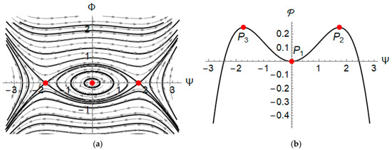
Figure 1.
Phase portrait for system (14) at and where (a) phase portrait and (b) potential function .
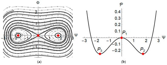
Figure 2.
Phase portrait for system (14) at and where (a) phase portrait and (b) potential function .
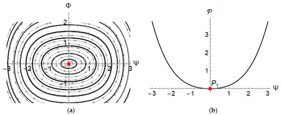
Figure 3.
Phase portrait for system (14) at and where (a) phase portrait and (b) potential function .
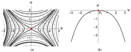
Figure 4.
Phase portrait for system (14) at and where (a) phase portrait and (b) potential function .
Figure 2a presents the phase portrait for system (14) when the dispersion coefficient μ = 1 and the velocity of the wave . Thus, we get three equilibrium points, , which is a saddle together with and , which are centers . This corresponds with Proposition 1(iv). Two homoclinic orbits are enclosed in the centers and and their source is saddle point . These homoclinic orbits correspond with the existence of the solitary wave solutions for the governing Equation (1). The periodic orbits that surround the centers and correspond with the existence of the periodic wave solutions for the governing Equation (1). In addition, there is also a family of super nonlinear periodic orbits enclosed in homoclinic and periodic orbits surrounding centers and . These periodic orbits correspond with the existence of the periodic wave solutions for the governing Equation (1). The potential function at the mentioned parameters is plotted in Figure 2b. Obviously, it has two local minima, and , which correspond to the centers and , respectively. Moreover, the local maxima P1 corresponds to the saddle equilibrium point .
In Figure 3, we depicted the phase portrait for system (14) at the dispersion coefficient μ = 1 and the velocity of the wave . According to Proposition 1(i), it appears to exist of unique equilibrium points, with being a center with periodic orbits enclosed in it (see Figure 3a). These periodic orbits correspond with the existence of periodic wave solutions for the governing Equation (1). Figure 3b shows the potential function at the same parameters and exhibits the existence of local minima for which corresponds to the center . Figure 4 displays no such behavior when the dispersion coefficient and the velocity of the wave (which makes system (14) have a unique saddle equilibrium point ) with special orbit passes through this saddle point. This indeed corresponds with the singular wave solution for the governing model (1). From the above discussion, we conclude that the existence of traveling wave solutions of the governing Equation (1) is related to the presence of homoclinic, heteroclinic, and periodic orbits that correspond to the equilibrium points of the dynamical system (14). In addition, the existence of such orbits directly depends on the dispersion coefficient and the velocity of the wave .
4. Traveling Wave Solutions
In the previous section we explained the existence of the traveling wave solution for the time-fractional mKdV-ZK Equation (1). In this section we extract and create some of these solutions using a suitable expansion for the wave profile that satisfies the integer-order ordinary differential Equation (13). We try to construct kink, solitary (bright and dark), and singular wave solutions for the time-fractional mKdV-ZK Equation (1).
4.1. Kink Wave Solutions
According to the above discussion, if the dispersion coefficient and the velocity of the wave , then the governing Equation (1) has kink wave solutions that correspond to the heteroclinic orbits as shown in Figure 1. It should be noted in this case that the negative dispersion is accompanied by a negative wave velocity, which indicates a negative energy flux. To construct these solutions, we consider the wave profile written as:
where the constants and will be determined. After substitution of the expression in (21) into integer-order ordinary differential Equation (13) and solving the algebraic system that was generated from making the coefficients of the independent terms to be zero, the wave profile reads as:
Therefore, the kink wave solution for the time-fractional mKdV-ZK Equation (1) is inferred as:
where and . The potential electric field is the amount of work energy that we need to stir an electric unit charge from a reference point in an electric field to a specific point. From line integrals, the electric potential in the electric field at a point can be written as:
where is an arbitrary path from a fixed reference point to . Utilizing the gradient theorem, we get:
According to the Maxwell–Faraday equation, a time-varying magnetic field escorts a non-conservative and spatially varying electric field. The magnetic field can be revealed using the electric field throughout the Maxwell–Faraday Equation:
where is the curl operator. Upon the obtained results in (23) and using (25), the corresponding electric fields to the electric field potentials (23) can be written as:
The obtained electric fields in (27) can be used in (26) to obtain the corresponding magnetic fields. Moreover, we can infer the difference between the density number of positrons of equal temperatures and hot electrons as follows:
The obtained wave profiles in (22) are plotted and shown in Figure 5 at the dispersion coefficient and the velocity of the wave υ = −1. We note that the wave profile is an anti-kink wave, such that the limit of the when approaches (see Figure 5a). In Figure 5b, we present the kink wave profile that has an opposite behavior of where the limit of the approaches when .
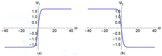
Figure 5.
The behavior of the wave profile in (22) at the dispersion coefficient and the velocity of the wave where (a) anti-kink wave solution and (b) kink wave solution .
We studied the amount of change for the anti-kink wave solution concerning the wave velocity and the dispersion coefficient . The conclusion is that if the wave velocity decreases, then the amplitude of the wave increases. For example, the limit of the when approaches at the wave velocity , while at the wave velocity , the limit of the approaches when (see Figure 6a). The anti-kink wave solution was affected by the change in the dispersion coefficient (see Figure 6b). We notice that the amplitude of the wave decreased when the dispersion coefficient μ decreased from to , whereas the limit of the when approaches at the dispersion coefficient , while at the dispersion coefficient , the limit of the approaches when . Therefore, a wane in the dispersion coefficient is accompanied by a flourish in the electric field potential.
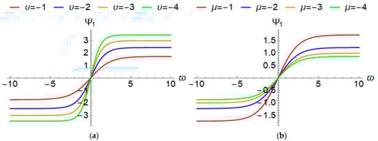
Figure 6.
Effect of the dispersion coefficient and the velocity of the wave on the behavior of the kink wave solution in (22) where (a) the dispersion coefficient and (b) the velocity of the wave .
The surface of the obtained kink wave solution in (23) is shown in Figure 7 at the dispersion coefficient and the wave velocity . We depicted concerning the independent variable and the time variable in a three-dimension plot in Figure 7a, while in Figure 7b we show a two-dimension plot of the behavior of concerning the independent variable at same parameters when the time variable . The limit of the kink solution under these parameters approaches when .
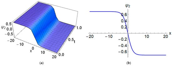
Figure 7.
The kink wave solution in (23) at the dispersion coefficient , the velocity of the wave , and the fractional derivative order where (a) 3D plot (b) 2D plot.
The fractional derivative affects the behavior of the traveling wave solutions, but unfortunately, there is no specific and theoretical description of this impact. Therefore, we depicted the inferred kink wave solution in (23) when the fractional derivative was considered with different orders in Figure 8, where the dispersion coefficient and the wave velocity were fixed at and , respectively. After studying and analyzing Figure 8, we found that the impact of the fractional derivative enhanced when the time variable increased. To illustrate our conclusion, let us consider Figure 8a when the time variable . The -intersection for the kink wave solution when (in red) and (in blue) approaches and , respectively. Thus, the gap between the two intersection points approaches . In Figure 8b, the time variable and the -intersection for the kink wave solution when (in red) and (in blue) approaches and , respectively. Hence, the gap between the two intersection points approaches . The same discussion applies to Figure 8c,d. It is worth mentioning that the limit of the kink solution does not vary by varying the fractional derivative order and it approaches when . Moreover, we notice from Figure 8 that the kink wave solution retracts left when the time variable grows. An example of this can be seen at the x-intersection for the kink wave solution when (in red) at the time variable , and 10 that we found approaches , and , respectively.
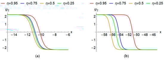
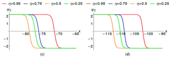
Figure 8.
Effect of the fractional derivative on the behavior of the kink wave solution in (23) at the dispersion coefficient , the velocity of the wave and where: (a) ; (b) ; (c) ; (d) .
4.2. Solitary Wave Solutions
As previously mentioned, the solitary wave solutions for the governing Equation (1) lead to homoclinic orbits within the dynamic system (14). In Section 3, we found that when the dispersion coefficient and the wave velocity, there are two centers and a unique saddle equilibrium point together with two homoclinic orbits, which use the saddle point as their source, and these orbits surrounded the centers. This case deals with positive group-velocity dispersion, meaning that the wave with a short length moves slower than the wave with a long length. The aim of this section is to establish solitary wave solutions for the time-fractional mKdV-ZK Equation (1) and provide the physical interpolation for these solutions to understand its behavior in certain statuses. We will construct solitary wave solutions involving the hyperbolic function using two different forms. Let us consider the solution of the integer-order ordinary differential Equation (12) which can be written as:
where the constants and are to be determined. Utilize the expression of the wave profile (29) into the integer-order ordinary differential Equation (12) and use some simplification, then consider the coefficients of the independent term to be zero to yield an algebraic system involving the constants , and the wave speed . Based on the solutions of the obtained algebraic system, we can write the solitary solutions for the integer-order ordinary differential Equation (12) in the form:
provided that and . These are two solitary wave solutions for the integer-order ordinary differential Equation (12) using direct substitution. Consequently, the solitary wave solutions for the time-fractional mKdV-ZK Equation (1) is inferred to be:
According to these results and using (25), the corresponding electric fields to the electric field potentials (31) can be written as:
The obtained electric fields in (32) can be used in (26) to obtain the corresponding magnetic fields. Moreover, we can infer the difference between the number density of positrons with equal temperatures and hot electrons as follows:
The explored wave profile in (30) is depicted in Figure 9 with the dispersion coefficient and the wave velocity. Figure 9a appears as a solitary wave with a crest that has an absolute maxima of , while Figure 9b shows a solitary wave with trough that has an absolute minima of . Obviously, the limit of as approaches zero.
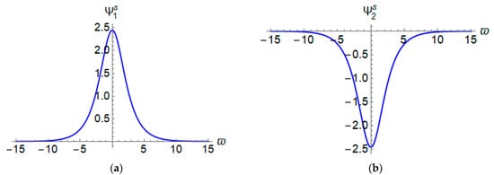
Figure 9.
The behavior of the wave profile in (30) at the dispersion coefficient and the velocity of the wave where (a) solitary crest wave solution and (b) solitary trough wave solution .
We studied the impact of the wave velocity and the dispersion coefficient on the solitary crest wave in (30). We obtained that the amplitude of the wave increases when the wave velocity increases, while the amplitude of the wave displays the opposite behavior when it is affected by the dispersion coefficient (see Figure 10). For instance, the absolute maxima for in Figure 10a at and was and , respectively. Moreover, we note that the effect of the wave velocity on the amplitude of the solitary crest wave makes it shrink whenever the wave velocity continues to increase. Figure 10b presents the impact of the dispersion coefficient , when its value changes from to , on the solitary crest wave solution with a fixed wave velocity of . We notice that a raise of the dispersion coefficient be accompanied by a fading of the electric field potential.
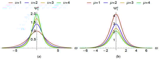
Figure 10.
Effect of the dispersion coefficient and the velocity of the wave on the behavior of the solitary crest wave solution in (30) where (a) the dispersion coefficient and (b) the velocity of the wave .
Figure 11 presents the surface of the obtained solitary wave solution in (31) at the dispersion coefficient and the wave velocity where the fractional derivative order . The absolute maxima for the solitary crest wave solution approaches . Figure 11a presents the three-dimensional plots for the obtained solution, while in (b) we depicted the obtained solution in two-dimensional plots where the time variable is considered at and .
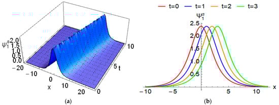
Figure 11.
The solitary crest wave solution in (31) at the dispersion coefficient , the velocity of the wave , and the fractional derivative order where (a) 3D plot (b) 2D plot.
The impact of the fractional derivative on the developed solitary trough wave solutions in (31) for the governing model (1) is displayed in Figure 12. We deemed the fractional derivative order to be , and when we depicted the inferred solution when the temporal variable and in Figure 12a,b, respectively. Obviously, the absolute minima at the trough for all showed solutions approaches at certain values for the spatial variable . In Figure 12a, we observe that the absolute minima when attained at , and where the fractional derivative orders were μ = 0.87, 0.73, 0.32, and , respectively. On the other hand, in Figure 12b when , the absolute minima was attained at , and where the fractional derivative orders were , and , respectively.
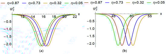
Figure 12.
Effect of the fractional derivative on the behavior of the solitary trough wave solution in (31) at the dispersion coefficient , the velocity of the wave, and where (a) and (b) .
4.3. Singular Wave Solution
Consider the dispersion coefficient and the velocity of the wave , then according to Figure 4, the time-fractional mKdV-ZK Equation (1) has a singular wave solution. To explore this solution, we assume that the integer-order ordinary differential Equation (12) has a solution in the form of:
where and are constants. To determine them, we insert the expression in (34) into integer-order ordinary differential Equation (12) and after some simplification and assigning the coefficients of the independent terms to zero, we obtain an algebraic system involving and . Solving the gained algebraic system leads us to the following solutions for the integer-order ordinary differential Equation (12):
Consequently, using the obtained solutions in (35) with aid of (11), the singular wave solutions for the time-fractional mKdV-ZK Equation (1) can be written as:
where and . According to these results and using (25), the electric fields corresponding to the electric field potentials (36) can be written as:
The obtained electric fields in (37) can be used in (26) to obtain the corresponding magnetic fields. Moreover, we can infer the difference between the number density of positrons with equal temperatures and hot electrons as follows:
Figure 13 shows the singular wave solution given in (35) when the dispersion coefficient and the velocity of the wave .
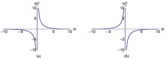
Figure 13.
The behavior of the singular wave profile in (35) at the dispersion coefficient and the velocity of the wave where (a) singular wave solution and (b) singular wave solution .
We studied the impact of varying the dispersion coefficient and the velocity of the wave υ on the obtained singular wave solutions in (35) and we depicted the results in Figure 14. In Figure 14a, we fixed the dispersion coefficient at and the velocity of the wave varies between the values of and . In Figure 14b we show the impact of varying the dispersion coefficient when the velocity of the wave is fixed at three.
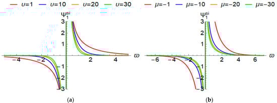
Figure 14.
Effect of the dispersion coefficient and the velocity of the wave on the behavior of the singular wave solution in (35) where (a) the dispersion coefficient and (b) the velocity of the wave .
The surface of the explored singular wave solution in (36) is presented in Figure 15a when the dispersion coefficient and the velocity of the wave at the fractional derivative order . Figure 15b shows the behavior of the singular wave solution in (36) in two-dimensions at same parameters. The fractional derivative plays an important role in the behavior of the obtained singular wave solution. Therefore, we depicted the singular wave solution at and when the order of the fractional derivative varied (see Figure 16).
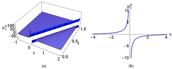
Figure 15.
The singular wave solution in (36) at the dispersion coefficient , the velocity of the wave , and the fractional order where (a) 3D plot and (b) 2D plot.
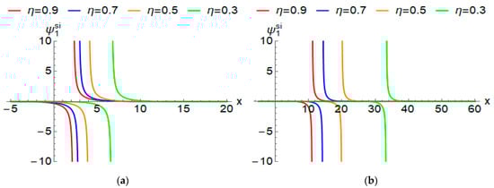
Figure 16.
Effect of the fractional derivative on the behavior of the singular wave solution in (36) at the dispersion coefficient , the velocity of the wave and where (a) and (b) .
5. Conclusions
This paper studied a significant and notable physical model, namely, the time-fractional mKdV-ZK equation of weakly nonlinear ion-acoustic waves in a magnetized electron–positron plasma. We considered the fractional derivative in the sense of the truncated M-fractional derivative. The governing model was reduced to an integer-order ordinary differential equation by a suitable traveling wave transformation with aid of the properties of the truncated M-fractional derivative. We obtained the corresponding dynamical system and introduced the bifurcation of its phase plane to ensure the existence of the traveling wave solutions for the governing model. The governing model’s solitary, kink, and singular wave solutions have been constructed using the ansatz method. The fractional mKdV-ZK equation has been studied by researchers using different approaches [31,32,33,34,35,36]. Our obtained results are in good agreement with other existing results. The novelty and significance of our results are due to showing the existence of the traveling wave solutions for the governing Equation (1) and introducing the bifurcation of nonlinear and super nonlinear ion-acoustic waves by utilizing phase plane analysis of the planar dynamical systems. In addition, the proposed method in this work is simple, effective, and applicable. The physical interpolation of the obtained solutions has been presented. In future work, we aim to study some other significant physical models in quantum plasmas and to investigate the traveling wave solutions for them and their applications.
Author Contributions
Conceptualization, M.A. and S.A.; methodology, M.A.-S.; formal analysis, S.A.; investigation, S.A.-O.; resources, S.A.-O.; writing—original draft preparation, M.A.; writing—review and editing, S.A.-O.; writing—review and editing, M.A.-S.; supervision, S.A.; project administration, S.A.-O.; funding acquisition, M.A.-S. All authors have read and agreed to the published version of the manuscript.
Funding
This work is supported by the Deanship for Research and Innovation, Ministry of Education in Saudi Arabia through the project number: IFP22UQU4282396DSR051.
Data Availability Statement
Not applicable.
Conflicts of Interest
The authors declare no conflict of interest.
References
- Rufai, O.R.; Bharuthram, R.; Singh, S.V.; Lakhina, G.S. Effect of excess superthermal hot electrons on finite amplitude ion-acoustic solitons and supersolitons in a magnetized auroral plasma. Phys. Plasmas 2015, 22, 102305. [Google Scholar] [CrossRef]
- Michel, F.C. Theory of pulsar magnetospheres. Rev. Mod. Phys. 1982, 54, 1. [Google Scholar] [CrossRef]
- Alinejad, H. Ion acoustic solitary waves in magnetized nonextensive electron-positron-ion plasma. Astrophys. Space Sci. 2013, 345, 85–90. [Google Scholar] [CrossRef]
- Ali, S.; Moslem, W.M.; Shukla, P.K.; Schlickeiser, R. Linear and nonlinear ion-acoustic waves in an unmagnetized electron-positron-ion quantum plasma. Phys. Plasmas 2007, 14, 082307. [Google Scholar] [CrossRef]
- Stenflo, L.; Shukla, P.K.; Yu, M.Y. Nonlinear propagation of electromagnetic waves in magnetized electron-positron plasmas. Astrophys. Space Sci. 1985, 117, 303–308. [Google Scholar] [CrossRef]
- Yinhua, C.; Yu, M.Y. Exact ion acoustic solitary waves in an impurity-containing magnetized plasma. Phys. Plasmas 1994, 1, 1868–1870. [Google Scholar] [CrossRef]
- Das, G.; Tagare, S.; Sarma, J. Quasipotential analysis for ion-acoustic solitary waves and double layers in plasmas. Planet. Space Sci. 1998, 46, 417–424. [Google Scholar] [CrossRef]
- Yadav, L.L.; Tiwari, R.S.; Maheshwari, K.P.; Sharma, S.R. Ion-acoustic nonlinear periodic waves in a two-electron-temperature plasma. Phys. Rev. E 1995, 52, 3045–3052. [Google Scholar] [CrossRef]
- Seadawy, A. Stability analysis for Zakharov-Kuznetsov equation of weakly nonlinear ion-acoustic waves in a plasma. Comput. Math. Appl. 2014, 67, 172–180. [Google Scholar] [CrossRef]
- Khater, A.H.; Callebaut, D.K.; Seadawy, A.R. Nonlinear Dispersive Instabilities in Kelvin–Helmholtz Magnetohydrodynamic Flows. Phys. Scr. 2003, 67, 340–349. [Google Scholar] [CrossRef]
- El-Labany, S.K.; Moslem, W.M.; El-Awady, E.I.; Shukla, P.K. Nonlinear dynamics associated with rotating magnetized electron–positron–ion plasmas. Phys. Lett. A 2010, 375, 159–164. [Google Scholar] [CrossRef]
- Verheest, F.; Mace, R.; Pillay, S.R.; Hellberg, M.A. Unified derivation of Korteweg-de Vries- Zakharov-Kuznetsov equations in multispecies plasmas. J. Phys. A Math. Gen. 2002, 35, 795–806. [Google Scholar] [CrossRef]
- Lazarus, I.J.; Bharuthram, R.; Hellberg, M.A. Modified Korteweg–de Vries–Zakharov-Kuznetsov solitons in symmetric two-temperature electron–positron plasmas. J. Plasma Phys. 2008, 74, 519–529. [Google Scholar] [CrossRef]
- Zhou, T.Y.; Tian, B.; Zhang, C.R.; Liu, S.H. Auto-Bäcklund transformations, bilinear forms, multiple-soliton, quasi-soliton and hybrid solutions of a (3+ 1)-dimensional modified Korteweg-de Vries-Zakharov-Kuznetsov equation in an electron-positron plasma. Eur. Phys. J. Plus 2022, 137, 912. [Google Scholar] [CrossRef]
- Rehman, H.; Seadawy, A.R.; Younis, M.; Rizvi, S.; Anwar, I.; Baber, M.; Althobaiti, A. Weakly nonlinear electron-acoustic waves in the fluid ions propagated via a (3+1)-dimensional generalized Korteweg–de-Vries–Zakharov-Kuznetsov equation in plasma physics. Results Phys. 2022, 33, 105069. [Google Scholar] [CrossRef]
- Younas, U.; Ren, J.; Baber, M.Z.; Yasin, M.W.; Shahzad, T. Ion-acoustic wave structures in the fluid ions modeled by higher dimensional generalized Korteweg-de Vries–Zakharov-Kuznetsov equation. J. Ocean Eng. Sci. 2022; in press. [Google Scholar] [CrossRef]
- Khater, M.M. Abundant stable and accurate solutions of the three-dimensional magnetized electron-positron plasma equations. J. Ocean Eng. Sci. 2022; in press. [Google Scholar] [CrossRef]
- Zureigat, H.; Al-Smadi, M.; Al-Khateeb, A.; Al-Omari, S.; Alhazmi, S.E. Fourth-Order Numerical Solutions for a Fuzzy Time-Fractional Convection–Diffusion Equation under Caputo Generalized Hukuhara Derivative. Fractal Fract. 2022, 7, 47. [Google Scholar] [CrossRef]
- Alabedalhadi, M.; Al-Smadi, M.; Al-Omari, S.; Karaca, Y.; Momani, S. New Bright and Kink Soliton Solutions for Fractional Complex Ginzburg–Landau Equation with Non-Local Nonlinearity Term. Fractal Fract. 2022, 6, 724. [Google Scholar] [CrossRef]
- Al-Smadi, M.; Abu Arqub, O.; Gaith, M. Numerical simulation of telegraph and Cattaneo fractional-type models using adaptive reproducing kernel framework. Math. Methods Appl. Sci. 2021, 44, 8472–8489. [Google Scholar] [CrossRef]
- Freihet, A.; Hasan, S.; Al-Smadi, M.; Gaith, M.; Momani, S. Construction of fractional power series solutions to fractional stiff system using residual functions algorithm. Adv. Differ. Equ. 2019, 2019, 95. [Google Scholar] [CrossRef]
- Freihet, A.; Hasan, S.; Alaroud, M.; Al-Smadi, M.; Ahmad, R.R.; Din, U.K.S. Toward computational algorithm for time-fractional Fokker–Planck models. Adv. Mech. Eng. 2019, 11, 1687814019881039. [Google Scholar] [CrossRef]
- Freihet, A.A.; Zuriqat, M. Analytical Solution of Fractional Burgers-Huxley Equations via Residual Power Series Method. Lobachevskii J. Math. 2019, 40, 174–182. [Google Scholar] [CrossRef]
- Alabedalhadi, M.; Al-Smadi, M.; Al-Omari, S.; Baleanu, D.; Momani, S. Structure of optical soliton solution for nonliear resonant space-time Schrödinger equation in conformable sense with full nonlinearity term. Phys. Scr. 2020, 95, 105215. [Google Scholar] [CrossRef]
- Shqair, M.; Alabedalhadi, M.; Al-Omari, S.; Al-Smadi, M. Abundant Exact Travelling Wave Solutions for a Fractional Massive Thirring Model Using Extended Jacobi Elliptic Function Method. Fractal Fract. 2022, 6, 252. [Google Scholar] [CrossRef]
- Alabedalhadi, M. Exact travelling wave solutions for nonlinear system of spatiotemporal fractional quantum mechanics equations. Alex. Eng. J. 2022, 61, 1033–1044. [Google Scholar] [CrossRef]
- Abdelhadi, M.; Alhazmi, S.E.; Al-Omari, S. On a Class of Partial Differential Equations and Their Solution via Local Fractional Integrals and Derivatives. Fractal Fract. 2022, 6, 210. [Google Scholar] [CrossRef]
- Alabedalhadi, M.; Al-Smadi, M.; Al-Omari, S.; Momani, S. New optical soliton solutions for coupled resonant Davey-Stewartson system with conformable operator. Opt. Quantum Electron. 2022, 54, 392. [Google Scholar] [CrossRef]
- Seadawy, A.R. Stability analysis solutions for nonlinear three-dimensional modified Korteweg–de Vries–Zakharov-Kuznetsov equation in a magnetized electron–positron plasma. Phys. A Stat. Mech. Its Appl. 2016, 455, 44–51. [Google Scholar] [CrossRef]
- Sahoo, S.; Ray, S.S. Improved fractional sub-equation method for (3+1) -dimensional generalized fractional KdV–Zakharov-Kuznetsov equations. Comput. Math. Appl. 2015, 70, 158–166. [Google Scholar] [CrossRef]
- Al-Ghafri, K.S.; Rezazadeh, H. Solitons and other solutions of (3+ 1)-dimensional space–time fractional modified KdV–Zakharov-Kuznetsov equation. Appl. Math. Nonlinear Sci. 2019, 4, 289–304. [Google Scholar] [CrossRef]
- Yel, G.; Sulaiman, T.A.; Baskonus, H.M. On the complex solutions to the (3+1)-dimensional conformable fractional modified KdV–Zakharov-Kuznetsov equation. Mod. Phys. Lett. B 2020, 34, 2050069. [Google Scholar] [CrossRef]
- Jin, Q.; Xia, T.; Wang, J. The Exact Solution of the Space-Time Fractional Modified Kdv-Zakharov-Kuznetsov Equation. J. Appl. Math. Phys. 2017, 5, 844–852. [Google Scholar] [CrossRef]
- Abdoon, M.A.; Hasan, F.L.; Taha, N.E. Computational Technique to Study Analytical Solutions to the Fractional Modified KDV-Zakharov-Kuznetsov Equation. Abstr. Appl. Anal. 2022, 2022, 2162356. [Google Scholar] [CrossRef]
- Sahoo, S.; Ray, S.S. Analysis of Lie symmetries with conservation laws for the (3+1) dimensional time-fractional mKdV-ZK equation in ion-acoustic waves. Nonlinear Dyn. 2017, 90, 1105–1113. [Google Scholar] [CrossRef]
- Alhejaili, W.; Salas, A.H.; El-Tantawy, S.A. Novel Approximations to the (Un)forced Pendulum–Cart System: Ansatz and KBM Methods. Mathematics 2022, 10, 2908. [Google Scholar] [CrossRef]
- Dong, S.-H. A New Approach to the Relativistic Schrödinger Equation with Central Potential: Ansatz Method. Int. J. Theor. Phys. 2001, 40, 559–567. [Google Scholar] [CrossRef]
- Sousa, J.V.D.C.; de Oliveira, E.C. On the local M-derivative. arXiv 2017, arXiv:1704.08186. [Google Scholar]
- Asjad, M.I.; Ullah, N.; Rehman, H.U.; Baleanu, D. Optical solitons for conformable space-time fractional nonlinear model. J. Math. Comput. Sci. 2022, 27, 28–41. [Google Scholar] [CrossRef]
- Asjad, M.I.; Ullah, N.; Rehman, H.U.; Gia, T.N. Novel soliton solutions to the Atangana–Baleanu fractional system of equations for the ISALWs. Open Phys. 2021, 19, 770–779. [Google Scholar] [CrossRef]
- Mohan Raja, M.; Vijayakumar, V. Optimal control results for Sobolev-type fractional mixed Volterra–Fredholm type integrodifferential equations of order 1< r < 2 with sectorial operators. Optim. Control Appl. Methods 2022, 43, 1314–1327. [Google Scholar]
- Raja, M.M.; Vijayakumar, V. Existence results for Caputo fractional mixed Volterra-Fredholm-type integrodifferential inclusions of order r∈(1, 2) with sectorial operators. Chaos Solitons Fractals 2022, 159, 112127. [Google Scholar] [CrossRef]
- Mohan Raja, M.; Shukla, A.; Nieto, J.J.; Vijayakumar, V.; Nisar, K.S. A note on the existence and controllability results for fractional integrodifferential inclusions of order r∈(1, 2] with impulses. Qual. Theory Dyn. Syst. 2022, 21, 1–41. [Google Scholar] [CrossRef]
- Ma, Y.K.; Raja, M.M.; Vijayakumar, V.; Shukla, A.; Albalawi, W.; Nisar, K.S. Existence and continuous dependence results for fractional evolution integrodifferential equations of order r∈(1, 2). Alex. Eng. J. 2022, 61, 9929–9939. [Google Scholar] [CrossRef]
- Ma, Y.-K.; Raja, M.M.; Nisar, K.S.; Shukla, A.; Vijayakumar, V. Results on controllability for Sobolev type fractional differential equations of order 1 < r < 2 with finite delay. AIMS Math. 2022, 7, 10215–10233. [Google Scholar] [CrossRef]
- Ortigueira, M.D.; Machado, J.T. What is a fractional derivative? J. Comput. Phys. 2015, 293, 4–13. [Google Scholar] [CrossRef]
- Katugampola, U.N. Correction to “What is a fractional derivative?” by Ortigueira and Machado [Journal of Computational Physics, volume 293, 15 July 2015, pages 4–13. Special issue on Fractional PDEs]. J. Comput. Phys. 2016, 321, 1255–1257. [Google Scholar] [CrossRef]
- Sousa, J.V.D.C.; De Oliveira, E.C. A New Truncated M-Fractional Derivative Type Unifying Some Fractional Derivative Types with Classical Properties. Int. J. Anal. Appl. 2018, 16, 83–96. [Google Scholar] [CrossRef]
- İlhan, E.; Kıymaz, İ.O. A generalization of truncated M-fractional derivative and applications to fractional differential equations. Appl. Math. Nonlinear Sci. 2020, 5, 171–188. [Google Scholar]
- Younis, M.; Rehman, H.U.; Iftikhar, M. Computational examples of a class of fractional order nonlinear evolution equations using modified extended direct algebraic method. J. Comput. Methods Sci. Eng. 2015, 15, 359–365. [Google Scholar] [CrossRef]
- Younis, M.; Rehman, H.U.; Iftikhar, M. Travelling wave solutions to some time–space nonlinear evolution equations. Appl. Math. Comput. 2014, 249, 81–88. [Google Scholar] [CrossRef]
- Rehman, H.U.; Inc, M.; Asjad, M.I.; Habib, A.; Munir, Q. New soliton solutions for the space-time fractional modified third order Korteweg–de Vries equation. J. Ocean Eng. Sci. 2022; in press. [Google Scholar] [CrossRef]
- Luo, D. Bifurcation Theory and Methods of Dynamical Systems; World Scientific: Singapore, 1997; Volume 15. [Google Scholar]
- Guckenheimer, J.; Holmes, P. Nonlinear Oscillations, Dynamical Systems, and Bifurcations of Vector Fields; Springer Science & Business Media: Berlin/Heidelberg, Germany, 2013; Volume 42. [Google Scholar]
- Tamang, J.; Saha, A. Bifurcations of small-amplitude supernonlinear waves of the mKdV and modified Gardner equations in a three-component electron-ion plasma. Phys. Plasmas 2020, 27, 012105. [Google Scholar] [CrossRef]
- Dubinov, A.E.; Kolotkov, D.Y.; Sazonkin, M.A. Nonlinear theory of ion-sound waves in a dusty electron-positron-ion plasma. Tech. Phys. 2012, 57, 585–593. [Google Scholar] [CrossRef]
- Seadawy, A.R. Stability analysis for two-dimensional ion-acoustic waves in quantum plasmas. Phys. Plasmas 2014, 21, 052107. [Google Scholar] [CrossRef]
- Iqbal, Z.; Shah, H.; Qureshi, M.; Masood, W.; Fayyaz, A. Nonlinear Dynamical Analysis of Drift Ion Acoustic Shock Waves in Electron-Positron-Ion Plasma with Adiabatic Trapping. Results Phys. 2022, 41, 105948. [Google Scholar] [CrossRef]


Disclaimer/Publisher’s Note: The statements, opinions and data contained in all publications are solely those of the individual author(s) and contributor(s) and not of MDPI and/or the editor(s). MDPI and/or the editor(s) disclaim responsibility for any injury to people or property resulting from any ideas, methods, instructions or products referred to in the content. |
© 2023 by the authors. Licensee MDPI, Basel, Switzerland. This article is an open access article distributed under the terms and conditions of the Creative Commons Attribution (CC BY) license (https://creativecommons.org/licenses/by/4.0/).