Abstract
Spatially offset Raman spectroscopy (SORS) is a non-invasive analytical technique that allows the analysis of samples through a container. This makes it an effective tool for studying food and beverage products, as it can measure the sample without being affected by the packaging or the container. In this study, a portable SORS equipment was used for the first time to analyse the alcoholic fermentation process of white wine. Different sample measurement arrangements were tested in order to determine the most effective method for monitoring the fermentation process and predicting key oenological parameters. The best results were obtained when the sample was directly measured through the glass container in which the fermentation was occurring. This allowed for the accurate monitoring of the process and the prediction of density and pH with a root mean square error of cross-validation (RMSECV) of 0.0029 g·L−1 and 0.04, respectively, and R2 values of 0.993 and 0.961 for density and pH, respectively. Additionally, the sources of variability depending on the measurement arrangements were studied using ANOVA-Simultaneous Component Analysis (ASCA).
1. Introduction
Winemaking is a dynamic biochemical process in which microorganisms and chemical compounds affect the course of the process and the properties and quality of the final product. The main reaction of the winemaking process is the transformation of sugars, basically glucose and fructose, into ethanol and carbon dioxide. This reaction is the basis of the alcoholic fermentation and occurs as part of yeast metabolism [1]. Moreover, due to secondary metabolism pathways other yeast metabolites are released at different concentrations, which are related to the organoleptic and physicochemical properties of the final product [1]. This process is highly sensitive to variations in chemical composition and external conditions (e.g., pH, sugar concentration or temperature), which could even lead to stuck or sluggish fermentations [2]. For this reason, close monitoring of the process is necessary to obtain real-time information that allows the necessary corrective measures to be taken in time to avoid a quality loss of the final product [3].
Currently, most wineries do not carry out exhaustive fermentation controls, but only rely on daily measurements of density and pH, as well as an organoleptic assessment by the oenologist [4]. However, the information provided by these parameters is not sufficient when abnormal fermentation behaviour appears and the decisions to be made depend on the results of more complex analyses, usually performed at-line or in external laboratories. This implies a delay in obtaining information and, therefore, in the application of corrective measures [5]. This delay can be a big problem if these actions are applied once the unwanted chemical substances have already impacted the organoleptic properties of the final product [6]. In this context, Process Analytical Technologies (PAT) are increasingly used, as they allow product quality to be assured through real-time measurements throughout the process [7]. Among the technologies, vibrational spectroscopy is frequently used in the food and beverage industries as it brings together several positive aspects: it allows obtaining information of each molecule in the matrix; it is sustainable, eco-friendly and requires minimal or no sample processing [5].
Near-infrared (NIR) and Mid-infrared (MIR) spectroscopies have already been used to monitor fermentation [8,9] and even to successfully detect deviations of the process [10,11]. However, these technologies have drawbacks in their application, such as the complexity of the signal in the case of NIR, as a consequence of weak overtones and combination bands; and the high MIR absorption of water bonds that make the use of special sampling devices mandatory to overcome signal saturation [12]. Raman spectroscopy could overcome these drawbacks as water bonds do not produce signal saturation and this spectroscopy produces sharp peaks that can be associated to specific bonds [12,13]. Even with these advantages it has rarely been used in on-line wine monitoring [14], mainly due to the fact that Raman spectroscopy is reliant on transparency of containers for the analysis of the sample contained within.
Nowadays, with Spatially Offset Raman Spectroscopy (SORS) it is possible to acquire Raman signals through many millimeters of different materials, allowing the analysis of the sample through barriers such as plastic, glass, paper, etc. The main characteristic of this type of measurement is that, unlike conventional Raman, the irradiation of the laser (excitation) and the collection of light do not coincide geometrically, but rather a spatially displaced measurement is performed. Therefore, since excitation and detection are spatially separate, a balanced subtraction of the two measurements creates a clean spectrum of the material contained [15,16]. This makes SORS a non-invasive, non-destructive technique that does not require sample preparation [17] and, thanks to the availability of commercial portable equipment, it has become of great interest as a tool for process quality control.
The aim of this research is to evaluate the use of a portable spatially offset Raman spectrophotometer (SORS) as a monitoring tool for wine alcoholic fermentation. Different sample measurement configurations were tested to assess the performance of the Raman spectrophotometer. Principal Component Analysis (PCA), Partial Least Squares Regression (PLSR) and ANOVA-Simultaneous Component Analysis (ASCA) were used to monitor the process, predict the main oenological parameters and study the sources of variability in Raman spectra.
2. Material and Methods
2.1. Fermentation Samples
Four alcoholic fermentations were carried out at small-scale (microfermentations) into 2.0 L glass cylindrical containers. White must from the dilution of a commercial concentrated must was used. The concentrated white must (Julián Soler S.A., Cuenca, Spain) was stored at −20 °C to avoid any biochemical or chemical evolution. 24 h before its use it was kept at 4 °C to defrost it. Then it was diluted with MilliQ water to adjust the sugar concentration to 200 g·L−1. To ensure a sufficient yeast assimilable nitrogen, the diluted must was supplemented with 0.30 g·L−1 of Actimabio* (Agrovin S.A., Ciudad Real, Spain) and ENOVIT® (Spindall S.A.R.L., Gretz Armainvilliers, France), respectively.
For each one of the four microvinifications (or biological replicates) 1,5 mL of diluted must was inoculated with commercial Saccharomyces cerevisiae yeast (Viniferm Revelación, Agrovin S.A.) ensuring an initial yeast population of 3·106 CFU·mL−1. Before inoculation, rehydration of the yeast was carried out following the suppliers’ instructions. All microvinifications were kept at a constant temperature of 20 °C until the end of alcoholic fermentation (that is, until the density was lower than 0.995 g·L−1, which is equivalent to a final sugar content under 1 g·L−1).
The alcoholic fermentation process was routinely controlled by measuring directly into the container density and pH, twice a day, with a portable densimeter (Densito2Go, Mettler Toledo, Columbus, OH, USA) and a portable pH meter with a 201 T electrode (7+ series portable pH-meter, XS Instruments, Italy). Both apparatus were calibrated once a day before use with a reference standard of 0.9982 g·ml−1 and two reference standards of pH 7.00 and 4.00, respectively. The densimeter cell and pH-meter electrode were thoroughly cleaned with deionized water before each new reading.
2.2. Raman Analysis
The Vaya Raman (Agilent, Santa Clara, CA, USA) portable SORS equipment was used in this research. This device uses a laser with an excitation wavelength of 830 nm to seek the suppression of fluorescence. The power of the laser was automatically adjusted by the spectrometer (taking into account the signal detected) to 450 mW reaching the maximum power available. The spectra were acquired in a range from 350 to 2000 cm−1. The equipment performs two consecutive measurements: with zero offset (parallel pathway of the laser and the detector) and with spatial offset (shift of 0.7 mm from the point of the laser incidence to the detector). After internal processing, the equipment records the SORS spectrum, which is the result of a scaled subtraction of the two measurements that provides a clean spectrum of the sample without the influence of the container layers.
The sample was measured from two different angles to study the performance of the SORS spectrophotometer in each case: directly next to the fermentation glass container in the horizontal plane (three equidistant points) and at the bottom of the container in the vertical plane. Furthermore, to detect the possible effect of turbidity, the samples were also measured directly next to the container in the horizontal plane after vigorous stirring. In every case, the SORS technology was applied to avoid the effect of the container. A scheme of the different analysis arrangements is represented in Figure 1.
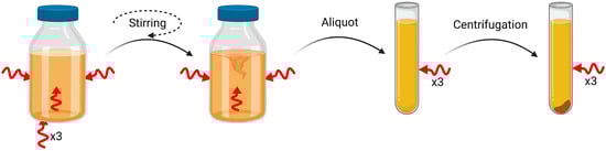
Figure 1.
Scheme of analysis arrangement. Each red arrow indicates the position where a Raman spectrometer was placed.
Aliquots of samples were also collected during the fermentation and analysed before and after centrifugation to obtain their spectra (without the influence of the container). Raman spectra of aliquots were obtained using a vial-mode configuration (Figure 1). The samples, contained in glass vials, were inserted into the sample holder inside the spectrometer and the light was focused on the sample to perform the scans.
Measurement times ranged from 30 s to 2 min per sample, while laser exposure times ranged from 0.5 to 2 s.
Each of the four microfermentation or biological replicates was analysed in triplicate in each measurement arrangement (represented in Figure 1) twice a day (with a twelve-hour gap) for seven consecutive days, which accounts for 14 sampling points for each biological replicate in each of the measurement arrangement.
2.3. Data analysis
2.3.1. Spectral Data Pre-Processing
Spectra were imported to MATLAB (R2021a, 9.10; MathWorks, Natick, MA, USA) to create five datasets (one for each analysis configuration) of 168 spectra (triplicates of 56 samples (4 biological replicates × 14 sampling points)), each consisting of 1651 wavenumbers. Multivariate analysis were performed using the PLS Toolbox (v9.0; Eigenvector Research Inc., Earglerock, CA, USA). Different pre-processing combinations were tested to overcome noise observed in the raw spectra: wavelet denoising (as implemented in Wavelet Toolbox v6.0), Savitzky-Golay (SG) smoothing and Standard Normal Variate (SNV), as implemented in the PLS Toolbox. The best spectral pre-processing combination to build all the multivariate models was wavelet denoising. Data were mean-centred before modelling.
2.3.2. Multivariate Data Analysis
PCA (Principal Component Analysis) is a well-known exploratory technique used to visualize the data (see e.g., [18] and references therein). It allows to detect groups and trends among samples and identify samples outliers, and to study relationships between the investigated variables. The algorithm decomposes the data into a set of new variables called Principal Components, which are linear combinations of the original variables orthogonal between them and retaining most of the information, and an error matrix, that contains non relevant information and the model noise. The projections of the samples onto the new space of Principal Components, known as scores, and the angles between the original variables and the principal components, known as loadings, can be plotted to reveal trends between samples and to help understand the sources of variability in the data. Partial Least Squares Regression (PLSR) was used to build models to predict density and pH [19]. For each measurement arrangement, an X data matrix (containing the sample spectra) and a Y data matrix (containing two columns, one for density and the other for pH), were used. Model evaluation was carried out using Cross-Validation as the validation method (ten random subsets iterated ten times) and calculating the Root Mean Squared Error of Cross-Validation (RMSECV) statistic (Equation (1)). This parameter describes how well the model predicts new samples using a cross validation strategy [12]. First, a partition of the set is performed, and each subset is excluded from the model building and then the excluded subset is predicted. This process is repeated until every subset is used:
are the densities or pHs predicted by the models, are the measured values (actual pH or density), and nt is the number of samples in the cross-validation set. RMSECV is an approximation of the average error to be expected in future predictions when the calibration model is applied to unknown samples.
Two statistical dimensionless parameters were used to assess the model’s predictive ability: Ratio of Performance to Deviation (RPD) and Range Error Ratio (RER) (Equations (2) and (3)) [20].
SD is the standard deviation of the reference parameters (pH and density), and ymax and ymin are the maximum and minimum vales of the reference parameters, respectively. Model predictions are considered good enough when RPD and RER are greater than two and ten, respectively.
Finally, Analysis of Variance (ANOVA)-Simultaneous Component Analysis (ASCA) was used to decompose the variability sources affecting the data. ASCA is a multivariate extension of ANOVA, which decomposes the variation in the data into the main effects and their binary combinations, obtained from a predefined experimental design [21]. In this study, three variability factors were considered: suspended yeast (stirring or no stirring in direct measurements; or centrifuge or no centrifuge in aliquot measurements), the alcoholic fermentation process itself and the biological replicates, and the interactions between them. The first step of ASCA requires partitioning the centred X matrix according to Equation (4):
where 1 is a vector of ones, mT is the average spectrum of the samples, Xsuspended yeast, Xalcoholic fermentation, Xbiological replicates are the matrices of the main factors, Xsuspended yeast × alcoholic fermentation, Xsuspendended yeast × biological replicate, Xalcoholic fermentation × biological replicate are the effect matrices for the binary interactions, and Xres is the residual matrix that collects the variability not taken into account in the experimental design. Each matrix is centred and contains the mean profiles of the samples corresponding to each factor or interaction level. Then, the matrices are decomposed using a technique called Simultaneous Component Analysis (SCA). It is important to note that SCA can be thought of as a form of principal component analysis that is constrained by ANOVA [21].
3. Results and Discussion
3.1. Evolution of the Alcoholic Fermentation
The correct progress of alcoholic fermentation was checked by two daily measurements of density and pH. The evolution of the density (Figure 2a) shows the typical sigmoidal trend [9], reaching the end of the fermentation in around 156 h. pH also exhibits the typical trend during alcoholic fermentation (Figure 2b) with a decrease until the midpoint of the tumultuous fermentation (at 76 h) due to the consumption of nitrogenous compounds and the release of organic acids. The second part of the alcoholic fermentation shows a slight increase in pH [1]. As all biological replicates behaved similarly, they were all considered as fermentations under control, and thus their Raman spectra were used for further analysis.
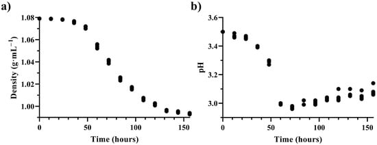
Figure 2.
Evolution of (a) density and (b) pH during alcoholic fermentation.
3.2. Raman Monitoring of the Alcoholic Fermentation
The first objective of the study was to establish the optimal arrangement for the acquisition of the sample signal, taking into consideration the angle between the Raman sensor and the sample container and the turbidity influence of the suspended yeast in the alcoholic fermentation matrix. For horizontal measurements through the fermentation glass container, three replicates were measured at three different side points of the container (always at the same three equidistant points) before and after manual stirring. Additionally, before stirring, a vertical measurement was performed at the bottom of the container, also in triplicate and always at the same point, to evaluate the effect of the yeast deposited at the bottom on the signal obtained.
To obtain a spectrum of the sample without the possible container interference, direct analysis of an aliquot of the fermentation samples was performed both before and after centrifugation.
To evaluate the influence of the container in the SORS spectra of the samples, an aliquot of each sampling point was analysed in a glass tube container provided by the manufacturer and that meets the provisions required for Raman spectroscopy. For this analysis, and to evaluate the effect of the suspended yeast on the signal as it was carried out for the direct analysis, measurements were performed before and after centrifugation. Three replicates of the sample of each microvinification at each sampling time were measured.
Figure 3 shows an example of the SORS spectra obtained at the beginning and at the end of the fermentation process. The main peaks in the first stage of alcoholic fermentation could be assigned to the vibration of different bonds belonging to the sugar molecules: 451 cm−1 for δ(C–C–O), 521 cm−1 for cyclic carbons, 1124 cm−1 for angular torsion and CH2 group at 1455 cm−1. Other important bands described in the alcoholic fermentation are C-O-H bending at 1424 cm−1, C-C stretching at 1130 cm−1 and C-O stretching at 1072 cm−1 [22]. As for the spectrum corresponding to the end of fermentation, the most characteristic band of ethanol assigned to the C-C stretching vibration around 880 cm−1 can be clearly seen [12,23].
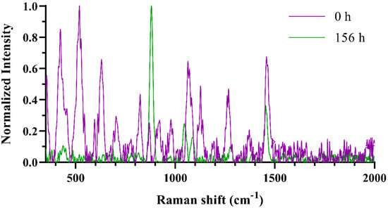
Figure 3.
SORS spectra of one biological replicate of alcoholic fermentation at the beginning (purple) and at the end (green) of the process.
To detect possible different trends depending on the arrangement used for signal acquisition, a PCA model was built for each configuration using the mean spectra of the three replicates. The dimensions of the matrices for each analysis configuration were 4 biological replicates × 14 time points × 1651 wavenumbers, which were unfolded to obtain two-dimensional matrices of 56 × 1651.
As shown in Figure 4, the evolution of the scores in the first principal component (PC) over time showed a process-related sigmoidal curve for each signal acquisition arrangement, except for the vertical measurement at the bottom of the sample container. This sigmoidal behaviour related to density evolution allows to stablish a monitoring of the process as stablished in our laboratory using mid-infrared spectroscopy and published in the following tutorial [9]. Regarding the process, after 96 h, a stabilization of the score values was observed, meaning that the first PC is not able to distinguish final stages of alcoholic fermentation, that end at hours 156 as previously mentioned (see paragraph 3.1). However, the second PC for “stirring” and “no stirring” PCA models showed an evolution over time in that period (Supplementary Materials Figure S1). This could be related to the final part of the consumption of sugars and the production of ethanol, as the loadings of this component are also related to sugars and ethanol. When looking at the reference samples (centrifuged and not centrifuged aliquots) they showed small differences in the score values of the first PC of the replicates at the end of the process, which could be related to biological variability. However, both configurations showed the same sigmoidal shape, and could be used to monitor the fermentation. Finally, in all cases the variance explained by the first PC ranges from 38.40 to 90.38% depending on the type of signal acquirement, showing a great variability compared to other variability sources in the spectra
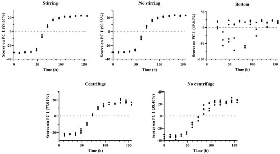
Figure 4.
Score plots of the first principal component of each PCA model for the different measurement configurations.
3.3. Prediction of Oenological Parameters
As both density and score values of the first PC show a sigmoidal evolution, we tried to predict density values along the alcoholic fermentation process by using PLSR. The five data matrices above described (56 samples × 1651 variables) were used in the experiment. The model performance parameters are shown in Table 1. RPD and RER were used to compare the performance of the prediction models. In addition, the number of LVs to be considered was optimized based on the curve of the RMSECV.

Table 1.
Density prediction results in each analysis configuration. LV: Latent Variables used in the PLSR models, RMSECV: Root Mean Square Error of Cross-Validations (expressed in g·mL−1), R2: determination coefficient, RPD: Ratio of Performance to Deviation, RER: Range Error Ratio.
As can be seen from the results, similar prediction models were obtained for “stirring” and “no stirring”, and between aliquot with and without centrifuge. The analysis at the bottom of the container, as expected by the inspection of the PCA scores in different PCs, was not able to predict density. This was also confirmed by looking at the loadings of the first LV of every measurement arrangement, with a large peak at 880 cm−1, being the major peak associated to ethanol (Figure S2a). Comparable results have been published in the literature for the prediction of sugars, as density is mainly related to the concentration of sugars in the fermenting must [12,14,22,23]. Both RPD and RER indicated that the best models are the ones of the direct analysis in the side of the container both before and after stirring. This is consistent with the literature stating that SORS coupled to chemometrics overcomes some Raman problems such as fluorescence [16]. In addition, regarding the present study we also attribute these better results to the greater representativeness of the fermentation process when analysing the whole fermentation sample than when taking only an aliquot.
Due to its importance in alcoholic fermentation monitoring, PLSR was also applied to predict pH. Following the same methodology as for density, the five data matrices (56 × 1651) were used to predict pH in every measurement arrangement. The quality parameters of the different models are summarized in Table 2.
Table 2.
pH prediction results in each analysis configuration. LV: Latent Variables used in the PLSR models, RMSECV: Root Mean Square Error of Cross-Validations, R2: determination coefficient, RPD: Ratio of Performance to Deviation, RER: Range Error Ratio.
As in the case of density, the performances of the pH prediction models were different for each signal acquisition configuration. The best performances were obtained with measurements performed at the container side, poorer performances were obtained when analysing the aliquots and the poorest prediction ability was obtained when measuring at the bottom of the container. For every predictive model, the loadings of the LVs (Figure S2b,c) are related to sugars, ethanol, and also a peak at 1760 cm−1 related to C=O stretching [16]. Regarding the quality parameters of the best models, the results are in agreement with the literature when using on-line conventional (non SORS) Raman spectroscopy [12,23], and proves the usefulness of SORS for monitoring the alcoholic fermentation.
Figure 5 shows the plots of predicted vs. measured values for the best models, using the spectra obtained from the measurements made directly on the side of the container without previous stirring.
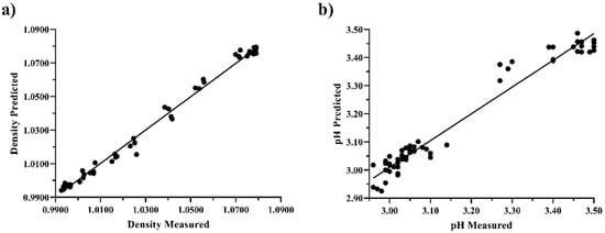
Figure 5.
Predicted vs. measured values for the best prediction models of (a) density (expressed in grams per millilitre) and (b) pH. Both models were calculated using spectra obtained from measurements without stirring.
3.4. Variability Sources
Two ASCA models were calculated to study the variability in the spectra associated to the presence of suspended yeast. Two extended matrices of 112 (56 samples × 2 measurement arrangements) × 1651 wavenumbers were used. ASCA results are expressed in terms of % Effect, which indicates the contribution of each factor to the matrix variability. A permutation test of 10,000 iterations was performed in each ASCA model to assess the significance of each factor (a p-value under 0.05 means the factor is significant) [24]. The ASCA results for the measurements made directly at the container side before and after stirring are summarized in Table 3.
Table 3.
ASCA results for the “stirring” and “no stirring” measurement arrangements, showing the percentage of variance (Effect (%)) for each factor and the p-value obtained from the permutation test. A p-value < 0.05 means the factor is significant.
As can be seen, the most relevant factor is the alcoholic fermentation process, which has already been shown to be very important in ATR-FTIR data of wine alcoholic fermentation [25]. This is consistent with the fact that during alcoholic fermentation yeast consumes approximately 200 g·L−1 of sugars and produces 13% ethanol, being the main source of variability in the data. As far as sample agitation is concerned, the results show that stirring the container to resuspend the yeast in the medium prior to the spectrum acquisition has no significant influence, making this step unnecessary. The biological replicate did not have a significant effect, but the interaction between biological replication and alcoholic fermentation process did. This could be explained by small differences in the speed of the process, with an effect of 2.08%.
The ASCA results for the measurements of the aliquot before and after centrifugation are summarized in Table 4.
Table 4.
ASCA results for centrifuge and no centrifuge measurement disposition, showing the percentage of variance (Effect (%)) for each factor and then p-value resulting of the permutation test. A p-value < 0.05 means the factor is significant.
ASCA results for aliquot measurements confirm that the alcoholic fermentation factor is again the greatest source of variability found in the data. However, in the case of the aliquot, the course of the alcoholic fermentation is different for the biological replicates, as the interaction between both factors was found large and significant. Alcoholic fermentation batches without centrifugation show more variability in each sampling point than batches with centrifugation. The standard deviation of the scores for each sampling point in Section 3.2 PCA range from 0.44 to 4.74 and 1.45 to 11.55 for aliquots with and without centrifugation, respectively. This result also explains why the interaction between centrifugation and alcoholic fermentation factors was also found large and significant. These ASCA results for aliquot analysis are in concordance with the results in Section 3.2 and Section 3.3, showing that centrifugation has a significant impact in the acquisition of Raman spectra, as in a short pathway with a priori no dispersion effects yeast may have caused light scattering.
4. Conclusions
The results presented demonstrate the ability of SORS to obtain the Raman spectra of wine alcoholic fermentation in a rapid, non-invasive and non-destructive way. Different measurement strategies were tested: through the container the fermentation was occurring with or without previous stirring and obtaining an aliquot to analysis in a Raman container. The variability associated to the different measurement configuration was assessed using ASCA, demonstrating that manual stirring has no impact in the performance of the SORS, but when dealing with an aliquot centrifugation has an impact due to the removal of suspended yeast. However, all measurement configurations, except those taken at the bottom of the container, successfully monitored the fermentation process and predicted density and pH as the main oenological parameters used in winemaking. The results obtained allow us to establish that SORS equipment could be used in the control of fermentation processes in an on-line configuration. Further research should be conducted to study the prediction of other oenological parameters of interest and the detection of process deviations, as well as the potential use of SORS for the analysis of other types of wine and alcoholic beverages.
Supplementary Materials
The following supporting information can be downloaded at: https://www.mdpi.com/article/10.3390/fermentation9020115/s1, Figure S1: Scores plots of the second Principal Component (PC2) of stirring and no stirring PCA model and Figure S2: Loading plot of density (first LV) and pH (first and second) PLSR model. Different colours mean different analytical methodologies (blue–Stirring, red–No stirring, green–Centrifuge, purple–No centrifuge).
Author Contributions
Conceptualization, R.B., B.G. and M.M.; methodology, D.S.-G.; software, D.S.-G. and J.E.; validation, B.G., R.B. and M.M.; formal analysis, R.B., B.G. and M.M.; investigation, D.S.-G. and J.E.; resources, L.A.; data curation, D.S.-G. and J.E.; writing—original draft preparation, D.S.-G.; writing—review and editing, R.B., B.G. and M.M.; visualization, D.S.-G. and J.E.; supervision, R.B., B.G. and M.M.; project administration, L.A.; funding acquisition, O.B. and R.B. All authors have read and agreed to the published version of the manuscript.
Funding
Grant PID2019-104269RR-C33 funded by MCIN/AEI/ 10.13039/501100011033. This publication has been possible with the support of the Secretaria d’Universitats i Recerca del Departament d’Empresa i Coneixement de la Generalitat de Catalunya (2020 FISDU 00221; Schorn-Garcia, D.). Grant URV Martí i Franqués—Banco Santander (2021PMF-BS-12).
Institutional Review Board Statement
Not applicable.
Informed Consent Statement
Not applicable.
Data Availability Statement
The data presented in this study are available on request from the corresponding author.
Acknowledgments
The authors would like to thank Agilent Technologies Spain for providing the portable Raman spectrophotometer used in this study. Graphical abstract was performed using BioRender.com.
Conflicts of Interest
The authors declare no conflict of interest.
References
- Ribereau-Gayon, P.; Dubourdieu, D.; Doneche, B.; Lonvaud, A. Handbook of Enology: The Microbiology of Wine and Vinifications, 2nd ed.; John Wiley & Sons: Hoboken, NJ, USA, 2006; Volume 1, pp. 1–497. [Google Scholar] [CrossRef]
- Urtubia, A.; Hernández, G.; Roger, J.M. Detection of Abnormal Fermentations in Wine Process by Multivariate Statistics and Pattern Recognition Techniques. J. Biotechnol. 2011, 159, 336–341. [Google Scholar] [CrossRef] [PubMed]
- Emparán, M.; Simpson, R.; Almonacid, S.; Teixeira, A.; Urtubia, A. Early Recognition of Problematic Wine Fermentations through Multivariate Data Analyses. Food Control 2012, 27, 248–253. [Google Scholar] [CrossRef]
- Bisson, L.F. Stuck and Sluggish Fermentations. Am. J. Enol. Vitic. 1999, 50, 107–119. [Google Scholar] [CrossRef]
- Cozzolino, D. Advantages, Opportunities, and Challenges of Vibrational Spectroscopy as Tool to Monitor Sustainable Food Systems. Food Anal. Methods 2022, 15, 1390–1396. [Google Scholar] [CrossRef]
- Cozzolino, D. State-of-the-Art Advantages and Drawbacks on the Application of Vibrational Spectroscopy to Monitor Alcoholic Fermentation (Beer and Wine). Appl. Spectrosc. Rev. 2016, 51, 282–297. [Google Scholar] [CrossRef]
- U.S. Department of Health and Human Services Food and Drug Administration. Guidance for Industry Guidance for Industry PAT —A Framework for Innovative Pharmaceutical Development, Manufacturing, and Quality Assurance; U.S. Department of Health and Human Services Food and Drug Administration: Silver Spring, MD, USA, 2004. [Google Scholar]
- di Egidio, V.; Sinelli, N.; Giovanelli, G.; Moles, A.; Casiraghi, E. NIR and MIR Spectroscopy as Rapid Methods to Monitor Red Wine Fermentation. Eur. Food Res. Technol. 2010, 230, 947–955. [Google Scholar] [CrossRef]
- Schorn-García, D.; Cavaglia, J.; Giussani, B.; Busto, O.; Aceña, L.; Mestres, M.; Boqué, R. ATR-MIR Spectroscopy as a Process Analytical Technology in Wine Alcoholic Fermentation—A Tutorial. Microchem. J. 2021, 166, 106215. [Google Scholar] [CrossRef]
- Cavaglia, J.; Schorn-García, D.; Giussani, B.; Ferré, J.; Busto, O.; Aceña, L.; Mestres, M.; Boqué, R. Monitoring Wine Fermentation Deviations Using an ATR-MIR Spectrometer and MSPC Charts. Chemom. Intell. Lab. Syst. 2020, 201, 104011. [Google Scholar] [CrossRef]
- Cavaglia, J.; Schorn-García, D.; Giussani, B.; Ferré, J.; Busto, O.; Aceña, L.; Mestres, M.; Boqué, R. ATR-MIR Spectroscopy and Multivariate Analysis in Alcoholic Fermentation Monitoring and Lactic Acid Bacteria Spoilage Detection. Food Control 2020, 109, 106947. [Google Scholar] [CrossRef]
- dos Santos, C.A.T.; Páscoa, R.N.M.J.; Porto, P.A.L.S.; Cerdeira, A.L.; González-Sáiz, J.M.; Pizarro, C.; Lopes, J.A. Raman Spectroscopy for Wine Analyses: A Comparison with near and Mid Infrared Spectroscopy. Talanta 2018, 186, 306–314. [Google Scholar] [CrossRef]
- Cozzolino, D. Sample Presentation, Sources of Error and Future Perspectives on the Application of Vibrational Spectroscopy in the Wine Industry. J. Sci. Food Agric. 2015, 95, 861–868. [Google Scholar] [CrossRef]
- Ávila, T.C.; Poppi, R.J.; Lunardi, I.; Tizei, P.A.G.; Pereira, G.A.G. Raman Spectroscopy and Chemometrics for On-Line Control of Glucose Fermentation by Saccharomyces Cerevisiae. Biotechnol. Prog. 2012, 28, 1598–1604. [Google Scholar] [CrossRef]
- Pérez-Beltran, C.H.; Pérez-Caballero, G.; Andrade, J.M.; Cuadros-Rodríguez, L.; Jiménez-Carvelo, A.M. Non-Targeted Spatially Offset Raman Spectroscopy-Based Vanguard Analytical Method to Authenticate Spirits: White Tequilas as a Case Study. Microchem. J. 2022, 183, 108126. [Google Scholar] [CrossRef]
- Jiménez-Carvelo, A.M.; Arroyo-Cerezo, A.; Bikrani, S.; Jia, W.; Koidis, A.; Cuadros-Rodríguez, L. Rapid and Non-Destructive Spatially Offset Raman Spectroscopic Analysis of Packaged Margarines and Fat-Spread Products. Microchem. J. 2022, 178, 107378. [Google Scholar] [CrossRef]
- Arroyo-Cerezo, A.; Jimenez-Carvelo, A.M.; González-Casado, A.; Koidis, A.; Cuadros-Rodríguez, L. Deep (Offset) Non-Invasive Raman Spectroscopy for the Evaluation of Food and Beverages-A Review. LWT-Food Sci. Technol. 2021, 149, 111822. [Google Scholar] [CrossRef]
- Esbensen, K.H.; Geladi, P. Principal Component Analysis: Concept, Geometrical Interpretation, Mathematical Background, Algorithms, History, Practice. Compr. Chemom. 2009, 2, 211–226. [Google Scholar] [CrossRef]
- Geladi, P.; Kowalski, B.R. Partial Least-Squares Regression: A Tutorial. Anal. Chim. Acta 1986, 185, 1–17. [Google Scholar] [CrossRef]
- Fearn, T. Assessing Calibrations: SEP, RPD, RER and R2. NIR News 2002, 13, 12–13. [Google Scholar] [CrossRef]
- Smilde, A.K.; Jansen, J.J.; Hoefsloot, H.C.J.; Lamers, R.J.A.N.; van der Greef, J.; Timmerman, M.E. ANOVA-Simultaneous Component Analysis (ASCA): A New Tool for Analyzing Designed Metabolomics Data. Bioinformatics 2005, 21, 3043–3048. [Google Scholar] [CrossRef]
- Wu, Z.; Xu, E.; Long, J.; Wang, F.; Xu, X.; Jin, Z.; Jiao, A. Measurement of Fermentation Parameters of Chinese Rice Wine Using Raman Spectroscopy Combined with Linear and Non-Linear Regression Methods. Food Control 2015, 56, 95–102. [Google Scholar] [CrossRef]
- Fuller, H.; Beaver, C.; Harbertson, J.; Jordão, M.; Michelle Wine Estates, S. Alcoholic Fermentation Monitoring and PH Prediction in Red and White Wine by Combining Spontaneous Raman Spectroscopy and Machine Learning Algorithms. Beverages 2021, 7, 78. [Google Scholar] [CrossRef]
- Bertinetto, C.; Engel, J.; Jansen, J. ANOVA Simultaneous Component Analysis: A Tutorial Review. Anal. Chim. Acta X 2020, 6, 100061. [Google Scholar] [CrossRef] [PubMed]
- Schorn-García, D.; Giussani, B.; Busto, O.; Aceña, L.; Mestres, M.; Boqué, R. Methodologies Based on ASCA to Elucidate the Influence of a Subprocess: Vinification as a Case of Study. J. Chemom. 2022, e3465. [Google Scholar] [CrossRef]
Disclaimer/Publisher’s Note: The statements, opinions and data contained in all publications are solely those of the individual author(s) and contributor(s) and not of MDPI and/or the editor(s). MDPI and/or the editor(s) disclaim responsibility for any injury to people or property resulting from any ideas, methods, instructions or products referred to in the content. |
© 2023 by the authors. Licensee MDPI, Basel, Switzerland. This article is an open access article distributed under the terms and conditions of the Creative Commons Attribution (CC BY) license (https://creativecommons.org/licenses/by/4.0/).