Big-But-Biased Data Analytics for Air Quality

Abstract

Air pollution is one of the big concerns for smart cities. The problem of applying big data analytics to sampling bias in the context of urban air quality is studied in this paper. A nonparametric estimator that incorporates kernel density estimation is used. When ignoring the biasing weight function, a small-sized simple random sample of the real population is assumed to be additionally observed. The general parameter considered is the mean of a transformation of the random variable of interest. A new bootstrap algorithm is used to approximate the mean squared error of the new estimator. Its minimization leads to an automatic bandwidth selector. The method is applied to a real data set concerning the levels of different pollutants in the urban air of the city of A Coruña (Galicia, NW Spain). Estimations for the mean and the cumulative distribution function of the level of ozone and nitrogen dioxide when the temperature is greater than or equal to 30 ${}^{\circ }$C based on 15 years of biased data are obtained.

1. Introduction

Making a city smart has emerged as a strategy to mitigate the challenges of urban population growth and fast urbanization, provinding better quality of life to its citizens [1]. The important role of Big Data Analytics and Information and Communication Technology in the development of smart cities initiatives is unquestionable [2]. There are many applications of Big Data in differents domains of smart cities, such as city planning, environment, sustainability, traffic management, transportation, security and education [3,4]. Some of the economic, environmental and social benefits and opportunities of using Big Data in smart city applications are detailed in [4].

1.1. Motivation

Despite the many advantages of applying Big Data Analytics to urban data, some authors have also identified some of its challenges, such as the importance of managing truthful and quality data [4,5]. Related to this issue, the idea that with enough data, numbers speak for themselves, often considered in this Big Data era, has already been discussed in [6,7,8]. This sentence reflects the doubtful notion that massive data sets always reflect objective and absolute truth. However, like any other human creation, data sets are not totally objective. Occasionally, a large sample is not completely representative of the population, but it is biased: Big-But-Biased Data (B3D). There are many situations where this happens, some of them in the context of smart cities.

An interesting source of big-but-biased data is the StreetBump smartphone app [9]. This app was created to help planning pothole patching in the city of Boston. The phone accelerometer and GPS data are registered by StreetBump while driving. Thus, bumps are detected and reported to the Boston traffic department to plan their repair and resource management. An important problem observed when using StreeBump was that people with lower income have a low rate of smartphone use. This rate is even lower for older residents, with low smartphone penetration. As a consequence, the data provided by StreetBump has a big sample size but it is a very biased sample of the population of potholes in Boston. As a consequence, the number of potholes in certain neighborhoods are underestimated, which causes a skewed management of resources.

The database of tweets generated by Hurricane Sandy is another interesting example cited by [9]. The data consists of more than 20 million tweets published between 27 October and 1 November 2012. Data analysis produced some expected findings, such as an increase in grocery shopping the night before the storm, and other surprising facts, such as nightlife increasing the day after the hurricane. However, the greatest number of tweets about Sandy came from Manhattan. This was due to the high level of smartphone owners and Twitter use in New York. Not many messages originated from the most affected areas by the catastrophe because the lack of electricity caused many problems with internet access and running out of battery in the hours after the storm. It is clear then that these data do not represent an unbiased sample of the population of tweets related to Sandy.

1.2. Similar Works

The present paper focuses on the domain of public health in smart cities; in particular, on urban air quality. Air pollution is one of the big concerns for smart cities. Information about real-time air quality is of great importance to protect humans from damage by air pollution [10].

There are many methods and works using Big Data Analytics to predict the air quality in smart cities. The authors in [11] compare several machine learning methods in order to choose the most suitable for predicting the ozone level in the Region of Murcia (Spain). In [12], four regression methods based on machine learning techniques are proposed to predict air pollution and compare their accuracy in terms of error rate and processing time, using multiple data sets. A novel deep learning model based on Long Short Term Memory networks is presented in [13] to make predictions about air quality in smart cities. In [14], the authors use the existing sensor networks in smart cities to create and promote alternative pollution-free routes across cities depending on the level of pollution in each zone and apply the study carried out to Madrid (Spain).

However, to the best of our knowledge, there is no published work dealing with the problem of sampling bias in Big Data Analytics for smart cities and air quality.

1.3. Content of The Paper

This paper deals with the problem of air quality in the context of big-but-biased data. The nonparametric estimation method proposed in [8] is applied. This method allows to estimate the mean of a transformation of a continuous population, which includes as special cases the mean of the population and any other moment, the cumulative distribution function and the characteristic function.

Section 2 introduces the problem and shows the density-based nonparametric estimator used. A new bootstrap algorithm is proposed in Section 2.3 to estimate the mean squared error (MSE) of the estimator. Its minimization leads to a method for automatic bandwidth selection, which is a relevant practical problem. A real data set study is carried out in Section 3. It is a data set with information of different variables of interest about air quality in the city of A Coruña, Galicia, NW Spain. The mean and the cumulative distribution function of the level of ozone (O${}_3$) and nitrogen dioxide (NO${}_2$) when the temperature is greater than or equal to 30 ${}^{\circ }$C is estimated based on 15 years of big-but-biased data, using the approach proposed in [8]. Section 4 includes the main conclusions and future perspectives.

2. Materials and Methods

2.1. Urban Air Quality

According to the World Health Organization (WHO), air pollution kills an estimated number of seven million people worldwide every year, increasing deaths from stroke, chronic obstructive pulmonary disease, lung cancer, heart disease and acute respiratory infections [15].

Air quality control and management have been one of the priorities of the environmental policy of the City Council of A Coruña for several years. After conducting an emission analysis, four automatic air pollution control stations were installed in different points of the city, aimed at protecting human health.

The Air Quality Index (AQI) is a global indicator of the air quality of an area at a certain time of the day, based on data provided by air quality monitoring stations. The AQI is calculated from information related to different atmospheric pollutants: sulfur dioxide (SO${}_2$), nitrogen oxides (NO${}_2$ y NO_x), carbon monoxide (CO), tropospheric ozone (O${}_3$), benzene (C${}_6$H${}_6$) and airborne particulate matter, smaller than 10 micrometers in diameter (PM10) and smaller than 2.5 micrometers in diameter (PM$2.5$). The AQI value changes every hour depending on the values obtained by the real-time surveillance stations. In case the air quality is poor, those responsible for the surveillance network receive an alert by email, initiating the corresponding action protocol [16]. This paper focuses on the levels of two of these pollutants: ozone (O${}_3$) and nitrogen dioxide (NO${}_2$).

Ozone at ground level (tropospheric ozone) is formed by the reaction of pollutants such as nitrogen oxides and volatile organic compounds emitted by vehicles and industry. Solar radiation plays an important role in these reactions, since the reactions are photochemical in nature and require high temperatures to be effective. As a result, the highest levels of ozone pollution occur on sunny and hot days. Excessive ozone in the air can have a marked effect on human health. It can cause breathing problems, trigger asthma, reduce lung function and cause lung diseases [15,16].

Nitrogen dioxide is one of the most dangerous pollutants due to its toxic and irritating nature, which causes significant inflammation of the airways. In addition, it decomposes through light to form atomic oxygen, which is very reactive, and converts molecular oxygen into ozone. The major emissions of NO${}_2$ are of anthropogenic origin, through combustion processes as heating, power generation and engines in vehicles and ships. Nitrogen oxides mainly affect the respiratory system and can cause bronchitis and pneumonia as well as a lower resistance to respiratory tract infections [15,16].

Since high temperatures are related to high values of these pollutants, the problem of estimating their levels when the temperature is greater than or equal to 30 ${}^{\circ }$C is considered. To carry out this study, the bias correction method proposed in [8], whose good performance has already been tested, is used.

2.2. Bias Correction Method

The method for bias correction consists of applying the nonparametric estimation techniques proposed in [8]. These techniques allows to estimate the mean of a transformation of a continuous random variable, ${\mu }_v$, in a B3D context: using a sample of a large size generated from a distribution which is not the one we are interested in, but some biased version of it. This general parameter is defined by ${\mu }_v=\int v\left(x\right)f\left(x\right)dx$, where v is a known function, and includes as especial cases the mean of the population ($v\left(x\right)=x$) and any other moment ($v\left(x\right)=x^k$, for some $k>0$), the cumulative distribution function at a given point t ($v\left(x\right)=\mathbf{1}(x\le t)$) and also the characteristic function evaluated at a given value t ($v\left(x\right)=exp\left(itx\right)$), among many others.

Let us denote by $\mathbf{X}=(X_1,\dots ,X_n)$ a simple random sample (SRS) of size n from the underlying continuous population with cumulative distribution function F (density f). Let us assume in this B3D setup that the sample $\mathbf{X}$ cannot be observed but instead we observe a sample $\mathbf{Y}=(Y_1,\dots ,Y_N)$ of a much larger size ($N>>n$) from a biased distribution G (density g) different from F. It is assumed that the two distributions have a common support, $\mathcal{D}$, and there exists a positive biasing function, $w\left(x\right),\forall x\in \mathcal{D}$, such that $g\left(x\right)=w\left(x\right)f\left(x\right)\forall x\in \mathcal{D}$.

Of course, if the sample $\mathbf{X}$ were observed, the classical estimator for ${\mu }_v$, the $v\left(X\right)$-sample mean, would be available: $\overline{v\left(X\right)}=\frac{1}{n}{\sum }_{i=1}^{n}v\left(X_i\right)$. If $\mathbf{X}$ is not available and we only observe $\mathbf{Y}$, the relationship between f and g can be used to estimate ${\mu }_v$:

$$E\left(\frac{v\left(Y\right)}{w\left(Y\right)}\right)=\int \frac{v\left(y\right)}{w\left(y\right)}g\left(y\right)dy=\int v\left(y\right)f\left(y\right)dy={\mu }_v.$$

(1)

Using Equation (1), an unrealistic estimator, which can be only used in practice when the function w is known [7], can be defined:

$${\tilde{\mu }}_v^{\left(1\right)}=\frac{1}{N}\sum _{i=1}^N\frac{v\left(Y_i\right)}{w\left(Y_i\right)}=\frac{1}{N}\sum _{i=1}^N\frac{f\left(Y_i\right)v\left(Y_i\right)}{g\left(Y_i\right)}.$$

(2)

Since ${\tilde{\mu }}_v^{\left(1\right)}$ is the sample mean of the simple random sample $Z_i=v\left(Y_i\right)/w\left(Y_i\right),i=1,\dots ,n$, it can be proved that is an unbiased estimator of ${\mu }_v$, with normal asymptotic distribution and variance ${\sigma }_Z^2/N$, where ${\sigma }_Z^2=\int v{\left(x\right)}^{2}f{\left(x\right)}^{2}g{\left(x\right)}^{-1}dx-{\mu }_v^2$.

The estimator in (2) is a weighted average of the $v\left(Y\right)$-sample, but the sample weights $f\left(Y_i\right)/g\left(Y_i\right)$ do not sum up to 1. So, we can consider the empirical version of the expectation ratio

$$\frac{E\left(\frac{v\left(Y\right)}{w\left(Y\right)}\right)}{E\left(\frac{1}{w\left(Y\right)}\right)},$$

which is equal to ${\mu }_v$, since

$$\begin{array}{ccc}\hfill E\left(\frac{1}{w\left(Y\right)}\right)& =& \int \frac{1}{w\left(y\right)}g\left(y\right)dy=\int f\left(y\right)dy=1.\hfill \end{array}$$

Thus, a reasonable modification of ${\tilde{\mu }}_v^{\left(1\right)}$ is given by:

$${\tilde{\mu }}_v^{\left(2\right)}=\frac{{\displaystyle \frac{1}{N}\sum _{i=1}^N\frac{v\left(Y_i\right)}{w\left(Y_i\right)}}}{{\displaystyle \frac{1}{N}\sum _{i=1}^N\frac{1}{w\left(Y_i\right)}}}=\frac{{\displaystyle \frac{1}{N}\sum _{i=1}^N\frac{f\left(Y_i\right)v\left(Y_i\right)}{g\left(Y_i\right)}}}{{\displaystyle \frac{1}{N}\sum _{i=1}^N\frac{f\left(Y_i\right)}{g\left(Y_i\right)}}}.$$

(3)

In general, the estimators in (2) and (3) are impractical, since the biasing function, w, is unknown. However, estimating the densities involved, f and g, we could obtain completely observable versions of the estimators for the population mean, ${\tilde{\mu }}_v^{\left(1\right)}$ and ${\tilde{\mu }}_v^{\left(2\right)}$. This can be done by collecting information of both densities. Since the big and biased sample, $\mathbf{Y}=(Y_1,\dots ,Y_N)$, is already observed, the density g can be easily estimated. To estimate f, we assume that we also observe a simple random sample, $\mathbf{X}=(X_1,\dots ,X_n)$, of a much smaller sample size n ($n<<N$) of the real population F.

Of course, when having the sample $\mathbf{X}$, it is certainly possible to estimate ${\mu }_v$ based on it. However, when the sample size of $\mathbf{X}$ is small, the quality of estimators based on it may be poor, while estimating ${\mu }_v$ using $\mathbf{Y}$ will have a much smaller variance (although some bias) due to its much larger sample size.

The biasing function, w, can be easily estimated by replacing the underlying density functions f and g by the Parzen–Rosenblatt kernel density estimators [17,18]:

$$\begin{array}{ccc}\hfill {\widehat{f}}_h\left(x\right)& =& \frac{1}{n}\sum _{i=1}^n{K}_h\left(x-X_i\right)\hfill \\ \hfill {\widehat{g}}_b\left(x\right)& =& \frac{1}{N}\sum _{i=1}^N{K}_b\left(x-Y_i\right)\hfill \end{array}$$

where $K_h\left(u\right)=(1/h)K\left(u/h\right)$, K is a kernel function and h and b are two smoothing parameters. This results in the estimator: ${\widehat{w}}_{h,b}\left(x\right)={\widehat{g}}_b\left(x\right)/{\widehat{f}}_h\left(x\right).$

Plugging these estimators into (3) leads to an observable versions of ${\tilde{\mu }}_v^{\left(2\right)}$:

$${\widehat{\mu }}_v^{2,h,b}=\frac{{\displaystyle \frac{1}{N}\sum _{i=1}^N\frac{v\left(Y_i\right)}{{\widehat{w}}_{h,b}\left(Y_i\right)}}}{{\displaystyle \frac{1}{N}\sum _{i=1}^N\frac{1}{{\widehat{w}}_{h,b}\left(Y_i\right)}}}=\frac{{\displaystyle \frac{1}{N}\sum _{i=1}^{N}v\left(Y_i\right)\frac{{\widehat{f}}_h\left(Y_i\right)}{{\widehat{g}}_b\left(Y_i\right)}}}{{\displaystyle \frac{1}{N}\sum _{i=1}^N\frac{{\widehat{f}}_h\left(Y_i\right)}{{\widehat{g}}_b\left(Y_i\right)}}}.$$

(4)

In [8], the good performance of the estimator ${\widehat{\mu }}_v^{2,h,b}$ has been shown and its asymptotic properties have been obtained. The influence of the two smoothing parameters has also been studied, exhibiting a striking limit behaviour of their optimal values. From now on, ${\widehat{\mu }}^{2,h,b}$ denotes the estimator in (4) when considering the mean estimation problem, i.e., $v\left(x\right)=x$. Nevertheless, a pending issue in [8] is the automatic bandwidth selection, for which we propose the following method.

2.3. Bootstrap Algorithm

Minimizing in the bandwidths h and b some estimator of the MSE is a reasonable way to obtain an automatic bandwidth selection method. To do this, the following bootstrap algorithm for MSE estimation is proposed:

• The estimated densities ${\widehat{f}}_{h_{pil}}$ and ${\widehat{g}}_{b_{pil}}$, where $h_{pil}$ and $b_{pil}$ denote the pilot bandwidhts obtained from the rule-of-thumb method, are considered as the true population densities in the bootstrap world.
• Bootstrap resamples, ${\mathbf{X}}^{\ast }=(X_1^{\ast },\dots ,X_n^{\ast })$ and ${\mathbf{Y}}^{\ast }=(Y_1^{\ast },\dots ,Y_N^{\ast })$, of sizes n and N respectively, are obtained from the estimated densities ${\widehat{f}}_{h_{pil}}$ and ${\widehat{g}}_{b_{pil}}$ as follows:

  (a)

  $X_i^{\ast }={\psi }_i^{\ast }+h_{pil}·u_i$, where ${\psi }^{\ast }=({\psi }_1^{\ast },\dots ,{\psi }_n^{\ast })$ is a simple random sample obtained from the empirical distribution computed with the values $\mathbf{X}=(X_1,\dots ,X_n)$ and $u=(u_1,\dots ,u_n)$, with $u_i$ simulated from the density K (a $N(0,1)$ when considering a Gaussian kernel), for $i=1,\dots ,n$.

  (b)

  $Y_i^{\ast }={\eta }_i^{\ast }+b_{pil}·v_i$, where ${\eta }^{\ast }=({\eta }_1,\dots ,{\eta }_N)$ is a simple random sample obtained from the empirical distribution computed with the values $\mathbf{Y}=(Y_1,\dots ,Y_N)$ and $v=(v_1,\dots ,v_N)$, with $v_i$ simulated from the density K (a $N(0,1)$ when considering a Gaussian kernel), for $i=1,\dots ,N$.

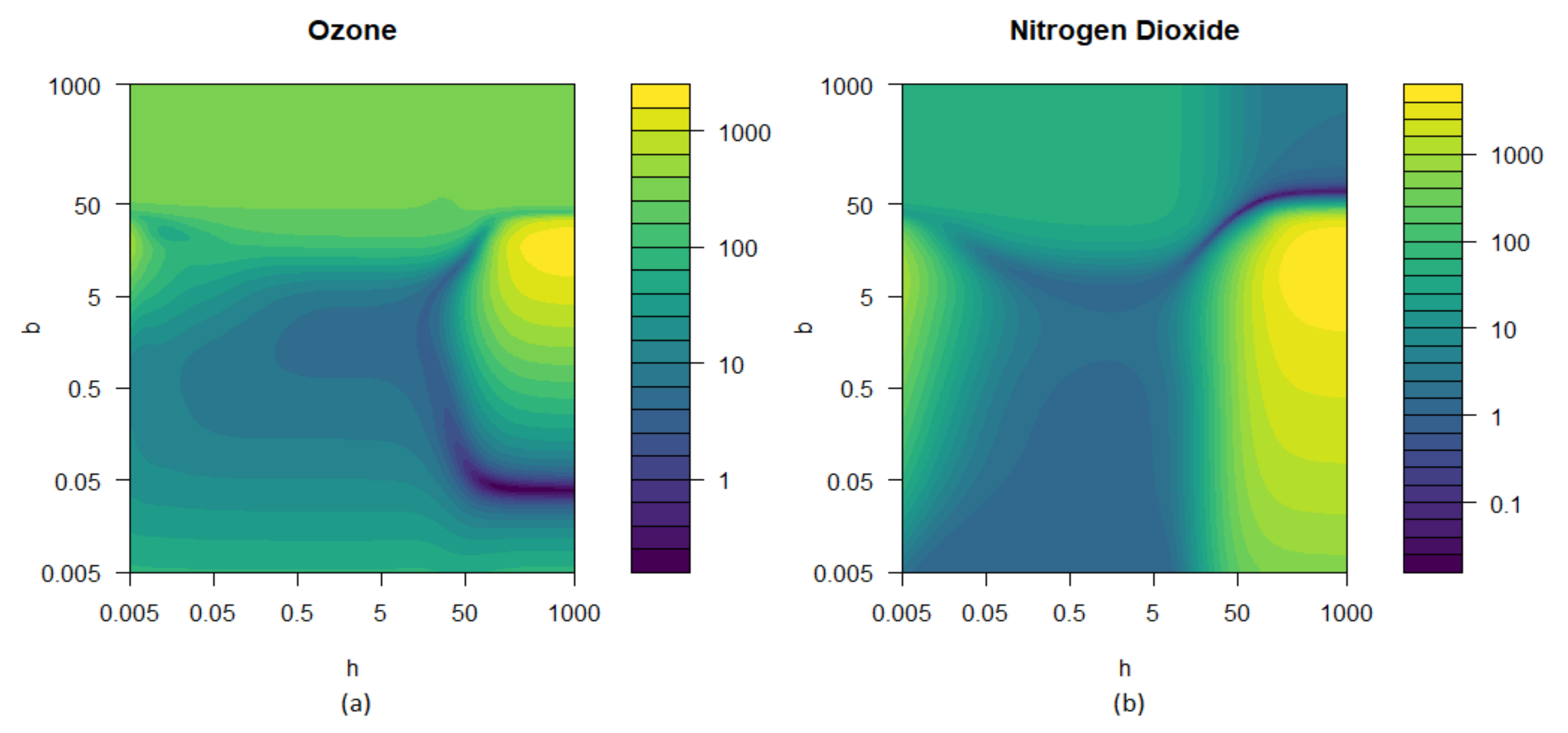
• The estimator ${\widehat{\mu }}^{2,h,b\ast }$ is implemented using the resamples ${\mathbf{X}}^{\ast }$ and ${\mathbf{Y}}^{\ast }$ and considering a very wide range of values for the smoothing parameters h and b.
• Steps 2 and 3 are repeated a large number of times, B, in order to obtain an approximation of the bootstrap mean squared error (MSE${}^{\ast }$) of the estimator,

  $$MS{E}^{\ast }(h,b)={\displaystyle \frac{1}{B}}\sum _{j=1}^B{\left({\widehat{\mu }}_j^{2,h,b\ast }-\overline{X}\right)}^2.$$
• The bandwidths $h^{\ast }$ and $b^{\ast }$ that minimize the function $MS{E}^{\ast }(h,b)$ are considered as bootstrap bandwidth selectors.

Since the MSE${}^{\ast }$ is not a robust measure, the presence of outliers could affect its value. In that case, other error measures could be considered, such as the bootstrap trimmed mean squared error (TMSE${}^{\ast }$), i.e., the trimmed mean to a certain proportion $\alpha$ (the mean excluding the proportion $\alpha$ of the highest values) of the squared errors, or the bootstrap median of the squared errors:

$$MeS{E}^{\ast }(h,b)=Median{\left({\widehat{\mu }}_j^{2,h,b\ast }-\overline{X}\right)}^2.$$

3. Results

The air quality data set mentioned in Section 1 is available in [16]. It consists of nearly 126 thousands hourly records about the temperature, measured in centigrades (${}^{\circ }$C), and the levels, in $\mathsf{\mu }$g/m${}^3$N, of O${}_3$ and NO${}_2$ in the urban air of A Coruña during the last 15 years. These data have been collected from the Santa Margarita station, one of the four automatic air pollution control stations in the city.

We are interested in estimating the mean level of ozone and nitrogen dioxide when the temperature is greater than or equal to 30 ${}^{\circ }$C, since high temperatures increase the level of these harmful pollutants in the air. For this purpose, we use (4), considering as Y the whole data set for the last 15 years ($N=$ 125,949 in the case of ozone and $N=$ 126,056 for nitrogen dioxide) and as X the data set with the level of ozone and nitrogen dioxide when the temperature is greater than or equal to 30 ${}^{\circ }$C in the last 15 years ($n=275$ and $n=267$, respectively). The difference between the sample sizes according to the variable considered is due to the missing data.

Figure 1 shows the density functions of the levels of ozone and nitrogen dioxide with temperatures greater than or equal to 30 ${}^{\circ }$C (dashed gray lines) when compared to the general levels of the last 15 years (solid black lines). The two densities are very similar for nitrogen dioxide, while they differ very much for ozone. The great difference depending on the temperature in the case of the ozone level was expected, since this connection has already been studied by several authors. Experiments performed in [19] show that high temperatures increase the ozone level, while the effect on nitrogen oxides is uncertain. In [20], not only is the relation between both variables analyzed, but also the effect it has on ozone-related mortality, concluding that high temperatures increase ozone level, which leads to a rise in the mortality rate. Furthermore, the authors in [21] warn about how the increase in the ozone level will negatively affect human health, agriculture and natural ecosystems due to climate change.

In fact, we can use the two sample Kolmogorov–Smirnov test [22,23] of equality of distributions to test for sampling bias. The p-values obtained (see

Table 1. p-values obtained in the two sample Kolmogorov–Smirnov (K–S) test of equality of distributions and in the two sample Student’s t-test of equality of means.

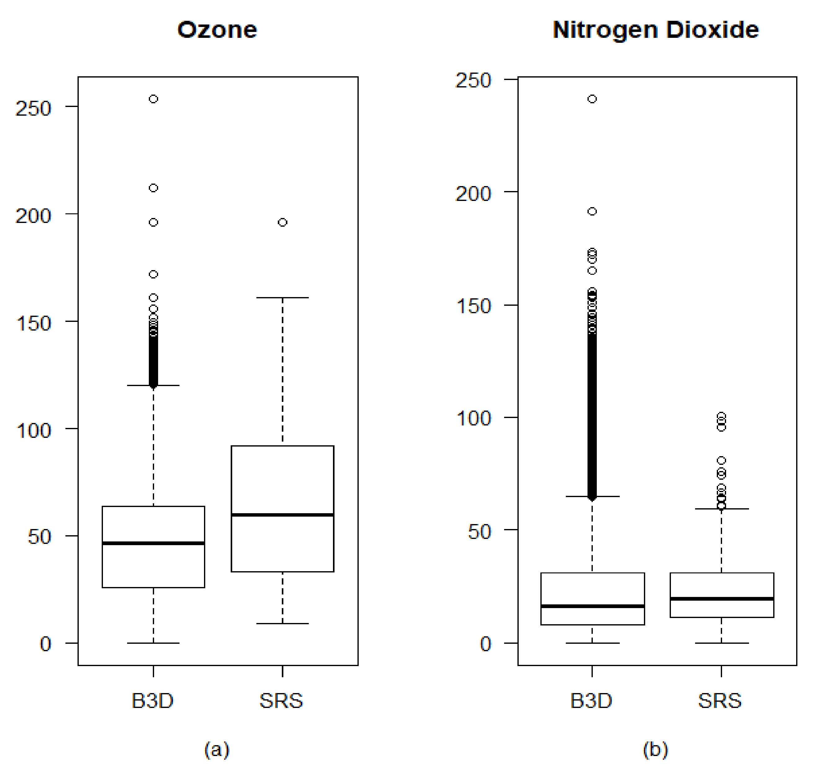
Variable	K–S test	$\overline{\mathit{X}}$	$\overline{\mathit{Y}}$	t-test
Ozone	<2.2 $\times {10}^{-16}$	64.44	45.35	<2.2 $\times {10}^{-16}$
Nitrogen dioxide	0.001064	23.88	22.28	0.1411

) allow to reject the null hypothesis in both cases, in favour of the presence of bias, but with a higher level of confidence in the case of ozone. Table 1 also shows the p-values obtained in the Student’s t-test, which allow to reject the equality of the means in the case of ozone with the usual levels of significance. However, the hypothesis of equal means for nitrogen dioxide is accepted using the t-test.

Figure 2 shows the presence of outliers, represented by circles on the upper side of the boxes, in the four samples involved. However, the bootstrap MSE will not be affected by these observations, since they are not measurement errors, but unusually high values of the levels of ozone and nitrogen dioxide in those particular hourly records.

In this context, we computed the values of $\overline{X}$ and $\overline{Y}$ in each case. As the sample mean of all the values for the two pollutants when the temperature is greater than or equal to 30 ${}^{\circ }$C is not available, the real $\mu$ is unknown. For this reason, in order to know which values of h and b provide a good performance of our estimator, we use the bootstrap bandwidth selection method presented in Section 2.3 above.

Figure 3 shows the bootstrap mean squared errors of the proposed estimator for bandwidth selection in the case of ozone and nitrogen dioxide, respectively. The color code on the right side of the figure refers to the MSE${}^{\ast }$ values of the estimator and indicates whether its value is very small (purple) or very high (yellow). This figure provides some estimate of the optimal values for the two bandwidths, those that minimize the MSE${}^{\ast }$. These values of h and b will be the ones used in the proposed method to estimate the mean level of both pollutants when the temperature is greater than or equal to 30 ${}^{\circ }$C. This figure also shows how relevant it is to properly select the smoothing parameter b; otherwise, the MSE${}^{\ast }$ would increase significantly. Once b has been chosen, it is also important to find a suitable h, although the range in which the estimator works correctly is wider for this bandwidth.

Table 2. Comparison of the full 15 years sample mean of the level of ozone and nitrogen dioxide with the mean of the analogous sample when the temperature is greater than or equal to 30 ${}^{\circ }$C and the proposed estimator $\widehat{\mu }$ for the values $h^{\ast }$ and $b^{\ast }$ obtained in the bootstrap implementation.

Variable	$\overline{\mathit{X}}$	$\overline{\mathit{Y}}$	${\mathit{h}}^{\ast }$	${\mathit{b}}^{\ast }$	${\widehat{\mathit{\mu }}}^{2,{\mathit{h}}^{\ast },{\mathit{b}}^{\ast }}$
Ozone	64.44	45.35	199.05	0.0397	67.94
Nitrogen dioxide	23.88	22.28	79.24	50	23.90

shows the estimated values, ${\widehat{\mu }}^{2,h,b}$, for the bootstrap bandwidth selectors $h^{\ast }$ and $b^{\ast }$. Considering the study performed in [8], the resulting bandwidths in the case of nitrogen dioxide are not surprising, since in situations of little bias it is expected to obtain high values for these parameters. More surprising is the case of ozone (more bias), in which we would expect to obtain small values for both parameters, which does not happen in the case of $h^{\ast }$.

As already mentioned, the proposed method allows to solve other problems, such as, for example, the estimation of the cumulative distribution function. Although this requires a specific bandwidth selection, for simplicity we will use those obtained by the bootstrap algorithm for mean estimation. Figure 4 shows the estimated distribution function using our proposed estimator. This figure exhibits important differences in the case of ozone, which was expected, since the more bias, the more the proposed estimator can benefit and beat the classical estimators based on the two samples.

4. Discussion and Conclusions

This paper deals with the problem of B3D Analytics for air quality in the context of smart cities. Analyzing air pollution and, in particular, ozone levels at high temperatures, are major challenges for smart cities, as some authors have already warned [19,20,21]. Several works using Big Data Analytics in this context have been analyzed [11,12,13,14], but none of them addresses one of the most relevant problems in this Big Data era: the presence of sampling bias. To analyze the pollution issue in a reliable and efficient way, it is essential to detect and correct its effect.

To correct the bias present in the real data set, we assume that a simple random sample ($\mathbf{X}$), of small size, from the real population is available. Of course, when having the sample $\mathbf{X}$, it is certainly possible to estimate ${\mu }_v$ based on it. However, when the sample size of $\mathbf{X}$ is small, the quality of the estimators based on it may be poor, while estimating ${\mu }_v$ using $\mathbf{Y}$ will have a much smaller variance (although some bias) due to its much larger sample size.

In addition to the application of the proposed method in [8] to an air quality data set, the problem of automatic bandwidth selection has been addressed through a bootstrap algorithm.

In the case of estimating the mean and the distribution function of the level of nitrogen dioxide, it is irrelevant to use the classical estimators based on the two samples or our proposed estimator, since the results are very similar. However, in the case of ozone, things change. Although the proposed estimator gives a similar value for the mean and an estimated distribution function close to the one obtained in the SRS case, the difference is big enough to take it into consideration. This is a relevant issue due to the already mentioned problems caused by high values of this pollutant. This is not surprising in view of Figure 1.

This research opens further interesting topics in the field, such as testing for sampling bias (using our own version of the two-sample Kolmogorov–Smirnov test, which includes the distinctive feature that the ratio of both samples sizes does not tend to a constant, since the size of the B3D sample tends to infinity faster than that of the SRS, or Bickel and Rosenblatt methods [24]); extensions to categorical settings (using, for instance, the estimators proposed in [25]); extensions to multidimensional X and Y; and including covariate dependence in the biasing weight.

References

- Chourabi, H.; Nam, T.; Walker, S.; Gil-Garcia, J.R.; Mellouli, S.; Nahon, K.; Pardo, T.A.; Scholl, H.J. Understanding smart cities: An integrative framework. In Proceedings of the 2012 45th Hawaii International Conference on System Sciences, Maui, HI, USA, 4–7 January 2012; pp. 2289–2297. [Google Scholar]
- Hashem, I.A.T.; Chang, V.; Anuar, N.B.; Adewole, K.; Yaqoob, I.; Gani, A.; Ahmed, E.; Chiroma, H. The role of big data in smart city. Int. J. Inf. Manag. 2016, 36, 748–758. [Google Scholar] [CrossRef]
- Osman, A.M.S. A novel big data analytics framework for smart cities. Future Gener. Comput. Syst. 2019, 91, 620–633. [Google Scholar] [CrossRef]
- Al Nuaimi, E.; Al Neyadi, H.; Mohamed, N.; Al-Jaroodi, J. Applications of big data to smart cities. J. Internet Serv. Appl. 2015, 6, 25. [Google Scholar] [CrossRef]
- Lim, C.; Kim, K.J.; Maglio, P.P. Smart cities with big data: Reference models, challenges, and considerations. Cities 2018, 82, 86–99. [Google Scholar] [CrossRef]
- Cao, R. Inferencia estadística con datos de gran volumen. Gac. Real Soc. Mat. Espa Nola 2015, 18, 393–417. [Google Scholar]
- Cao, R.; Borrajo, L. Nonparametric mean estimation for big-but-biased data. In The Mathematics of the Uncertain; Springer: Berlin/Heidelberg, Germany, 2018; pp. 55–65. [Google Scholar]
- Borrajo, L.; Cao, R. Nonparametric Estimation for Big-But-Biased Data. 2020, Unpublished Manuscript. Available online: http://dm.udc.es/modes/es/node/52 (accessed on 15 August 2020).
- Crawford, K. The hidden biases in big data. Harv. Bus. Rev. 2013, 1, 814. [Google Scholar]
- Zheng, Y.; Liu, F.; Hsieh, H.P. U-air: When urban air quality inference meets big data. In Proceedings of the 19th ACM SIGKDD International Conference on Knowledge Discovery and Data Mining, Chicago, IL, USA, 11–14 August 2013; pp. 1436–1444. [Google Scholar]
- Martínez-España, R.; Bueno-Crespo, A.; Timon-Perez, I.M.; Soto, J.A.; Ortega, A.M.; Cecilia, J.M. Air-Pollution Prediction in Smart Cities through Machine Learning Methods: A Case of Study in Murcia, Spain. J. UCS 2018, 24, 261–276. [Google Scholar]
- Ameer, S.; Shah, M.A.; Khan, A.; Song, H.; Maple, C.; Islam, S.U.; Asghar, M.N. Comparative analysis of machine learning techniques for predicting air quality in smart cities. IEEE Access 2019, 7, 128325–128338. [Google Scholar] [CrossRef]
- Kök, İ.; Şimşek, M.U.; Özdemir, S. A deep learning model for air quality prediction in smart cities. In Proceedings of the 2017 IEEE International Conference on Big Data (Big Data), Boston, MA, USA, 11–14 December 2017; pp. 1983–1990. [Google Scholar]
- Ramos, F.; Trilles, S.; Muñoz, A.; Huerta, J. Promoting pollution-free routes in smart cities using air quality sensor networks. Sensors 2018, 18, 2507. [Google Scholar] [CrossRef] [PubMed]
- World Health Organization (WHO). Air Pollution. Available online: http://www.who.int/airpollution/en/ (accessed on 12 August 2020).
- Ayuntamiento de A Coruña, Spain. Coruña Sostenible. Available online: http://coruna.es/infoambiental/ (accessed on 10 August 2020).
- Parzen, E. On estimation of a probability density function and mode. Ann. Math. Stat. 1962, 33, 1065–1076. [Google Scholar] [CrossRef]
- Rosenblatt, M. Remarks on some nonparametric estimates of a density function. Ann. Math. Stat. 1956, 27, 832–837. [Google Scholar] [CrossRef]
- Cardelino, C.; Chameides, W. Natural hydrocarbons, urbanization, and urban ozone. J. Geophys. Res. Atmos. 1990, 95, 13971–13979. [Google Scholar] [CrossRef]
- Jhun, I.; Fann, N.; Zanobetti, A.; Hubbell, B. Effect modification of ozone-related mortality risks by temperature in 97 US cities. Environ. Int. 2014, 73, 128–134. [Google Scholar] [CrossRef]
- Meleux, F.; Solmon, F.; Giorgi, F. Increase in summer European ozone amounts due to climate change. Atmos. Environ. 2007, 41, 7577–7587. [Google Scholar] [CrossRef]
- Kolmogorov, A. Sulla determinazione empirica di una legge di distribuzione. Inst. Ital. Attuari Giorn. 1933, 4, 83–91. [Google Scholar]
- Smirnov, N.V. Estimate of deviation between empirical distribution functions in two independent samples. Bull. Mosc. Univ. 1939, 2, 3–16. [Google Scholar]
- Bickel, P.J.; Rosenblatt, M. On some global measures of the deviations of density function estimates. Ann. Stat. 1973, 1, 1071–1095. [Google Scholar] [CrossRef]
- Li, Q.; Racine, J. Nonparametric estimation of distributions with categorical and continuous data. J. Multivar. Anal. 2003, 86, 266–292. [Google Scholar] [CrossRef]
Sample Availability: Data used in this paper and the script in R are available at http://dm.udc.es/modes/es/node/52. |