Article

Bagged Tree Based Frame-Wise Beforehand Prediction Approach for HEVC Intra-Coding Unit Partitioning

1
Information Security Center, State Key Laboratory of Networking and Switching Technology, Beijing University of Posts and Telecommunications, Beijing 100876, China
2
National Engineering Laboratory for Disaster Backup and Recovery, Beijing University of Posts and Telecommunications, Beijing 100876, China
3
Guizhou Provincial Key Laboratory of Public Big Data, Guizhou University, Guiyang 550025, China
*
Author to whom correspondence should be addressed.
Electronics 2020, 9(9), 1523; https://doi.org/10.3390/electronics9091523
Submission received: 21 August 2020 / Revised: 12 September 2020 / Accepted: 14 September 2020 / Published: 17 September 2020
(This article belongs to the Special Issue Multimedia Systems and Signal Processing)

Abstract

:
High Efficiency Video Coding (HEVC) has achieved about 50% bit-rates saving compared with its predecessor H.264 standard, while the encoding complexity increases dramatically. Due to the introduction of more flexible partition structures and more optional prediction directions, HEVC takes a brute force approach to find the optimal partitioning result which is much more time consuming. Therefore, this paper proposes a bagged trees based fast approach (BTFA) and focuses on the coding unit (CU) size decision for HEVC intra-coding. First, several key features of a target CU are extracted for three-output classifiers. Then, to avoid feature extraction and prediction time over head, our approach is designed frame-wisely, and the procedure is applied parallel with the encoding process. Using the adaptive threshold determination algorithm, our approach achieves 42.04% time saving with negligible 0.92% Bit-Distortion (BD)-rate loss. Furthermore, in order to calculate the optimal thresholds to balance BD-rate loss and complexity reduction, the neural network based mathematical fitting is added to BTFA, which is called the advanced bagged trees based fast approach (ABTFA). Finally, experimental results show that ABTFA achieves 47.87% time saving with only 0.96% BD-rate loss, which outperforms other state-of-the-art approaches.

1. Introduction

High Efficiency Video Coding (HEVC) is the state-of-the-art video coding standard. It was developed by the Joint Collaborative Team on Video Coding (JCT-VC) [1]. Compared with its predecessor H.264/Advanced Video Coding (AVC) [2], it implements more advanced encoding techniques, such as larger coding tree unit (CTU). It achieves about 50% bit-rate reduction while maintaining video quality. However it also increases the encoding complexity dramatically.
HEVC doubles the compression ratio by introducing many progressive encoding tools, such as more available prediction modes and more flexible coding unit (CU) partition structures [3]. It adopts a block-based hybrid coding framework and takes a recursive CU splitting strategy. In HEVC, the frames are firstly divided into nonoverlapped blocks in square shape called Coding Tree Unit (CTU) that can be as large as 64 × 64. Each CTU can be further divided into four smaller CUs in square shape. Depending on the frame characteristic, each of these smaller CUs can be further divided into new sub-CUs according to a quad-tree structure. The size of CUs can be supported from 64 × 64 to as small as 8 × 8. Once the size of a CU is decided, the CU can also be further partitioned into smaller units called the prediction units (PUs) which are used for pixels prediction and residuals calculation. In the case of intra-coding, PU can be as large as its root CU or as small as a 4 × 4 pixels block. An example of CTU splitting and corresponding quart-tree structures of CU and PU are shown in Figure 1. In Figure 1, CU partitions are presented with blue solid line while PU partitions are presented by red dash line. According to Figure 1, we can see that a CTU can be further partitioned into four depth levels, also we use the depth level to represent the CU size. Obviously, it is difficult and time-consuming to find the optimal size of the CUs and PUs from so many combinations of different sizes. HEVC uses a full rate-distortion optimization (RDO) strategy to traverse all the possible combinations (i.e., all different CU sizes) and selects the one with the minimum rate-distortion cost as the best [4]. The searching procedure for optimal CU size makes great effort to increase the compression ratio, but it also brings significant complexity increment. This drawback hinders its implementation in real-time applications, thus there is an urge for a fast CU size decision algorithm to reduce the encoding complexity of HEVC.
To address the above mentioned problem (i.e., the heavy burden caused by the searching for the optimal combination of CU sizes), many works designed fast CU size decision algorithms, which can be roughly classified to two main categories [5,6]. The first category includes the algorithms based on statistics-based heuristics [7,8]. The second category consists of the algorithms based on advanced machine learning techniques, such as Support Vector Machine (SVM) [9], Decision Trees [10], Bayesian method with conditional random fields [11] and Neural Networks [12,13]. Though some statistical information based fast algorithms can achieve a good performance [14,15], the statistical distributions and thresholds are different from sequence to sequence. Moreover, their performances are highly dependent on special video sequence. On the other hand, machine learning based methods can explore much more information automatically from video sequence. Many works have proved that machine learning based methods outperform other heuristics based ones [12,16,17].
However, machine learning based algorithms have some limitations. For example, SVM takes a heavy time burden on training and prediction [18]. Furthermore, most recent works use one or more SVMs on each depth to improve the precision [6,17], so that the training time is doubled. Neural network models are always large-scale and take a long time to train [19]. On the contrary, compared with SVM and neural network based approaches, decision tree based approaches can be trained much easier and take much less time to finish the prediction [20]. Besides, they are always small-scale and easy to be implemented. Furthermore, the existing machine learning based methods apply a pipeline strategy [6,9,17,19]. They always perform online prediction followed by different splitting process according to the prediction results, and it does not take advantage of intra-coding properties.
In this paper, we propose a frame-wise fast CU size decision algorithm for HEVC intra-coding by combining multiple decision trees. We not only design several novel features, but also propose an implementation method called the frame-wise beforehand prediction. Using this method, we can predict the splitting results of the next frame when the encoder is encoding the current frame. In this way, we can always carry out prediction in parallel before the target frame is being encoded, so called frame-wise beforehand prediction. In the proposed algorithm, only one bagged tree is applied to CU decision progress of all depth 0, 1, 2. It makes our algorithm faster and more convenient. Besides, this paper uses an adaptive threshold determination process on the classifier to compensate the loss of precision. Thus, based on machine learning and HEVC intra-coding properties, this paper finally generates bagged tree based fast algorithm for HEVC intra-coding with adaptive threshold determination (i.e., BTFA). However, BTFA can only find hazy thresholds and achieve a barely satisfactory performance. Aiming at achieving the best performance, this paper also employs neural network based mathematical fitting method upon BTFA to achieve a trade-off between distortion and complexity, which is called advanced bagged tree based fast intra-CU size determination algorithm (ABTFA). ABTFA is able to achieve an optimal result according to a certain constraint of Bit-Distortion (BD)-rate loss or time saving.
The key innovation and contributions of this paper are presented as follows:
  • Several novel and meaningful features are proposed. Especially, features designed based on Haar wavelet transform and interest points contribute a lot to the prediction performance. Besides, an importance rank of features is generated in the training phase of bagged tree models. The ranking process is very important for feature analysis and saves time.
  • A more general and accurate model is proposed. Different from traditional decision tree based methods, a more general and accurate bagged tree method is implied to CU partitioning problem. In particular, one bagged tree model is used for CUs of three sizes, i.e., 64 × 64, 32 × 32, 16 × 16.
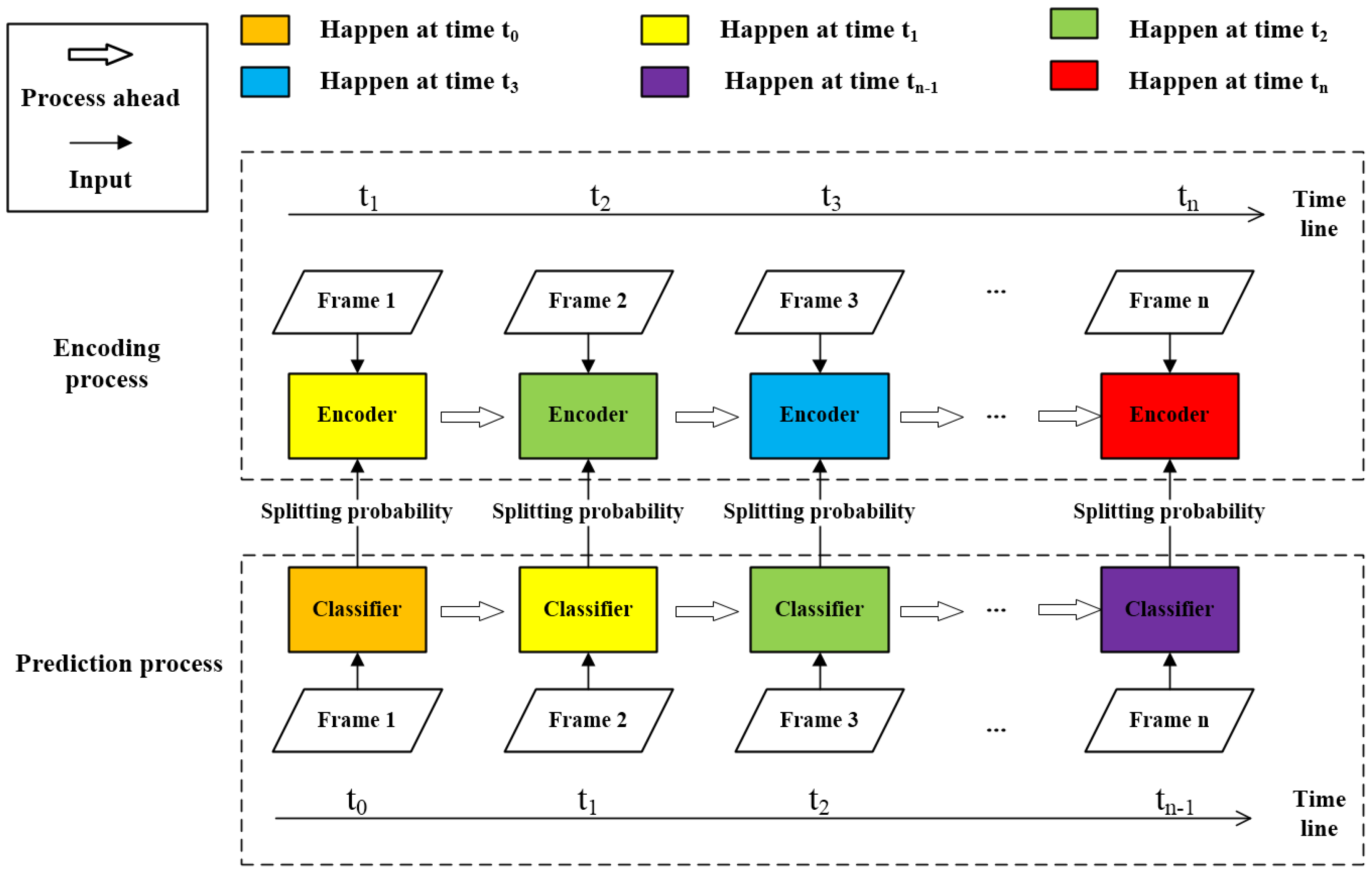
  • Parallel frame-wise prediction process is applied. This before-hand processing allows encoder to execute CU splitting directly according to the prediction results output ahead of schedule. So that the time spent on features extraction and prediction can be saved.
  • Advanced mathematical fitting technique is employed. In this paper, to calculate optimal thresholds under a certain constraint, neural network is used to find the best value of thresholds which are needed for CU splitting label prediction. In this way, the prediction accuracy is improved, and the proposed ABTFA has the best performance under a certain constraint of BD-rate loss or time saving.
This paper is organized as follows. Section 2 describes related works of fast CU partitioning techniques. Fundamental knowledge of bagged tree model is presented in Section 3. The proposed bagged tree based fast algorithm for intra-CU partitioning, i.e., BTFA, is presented in Section 4. The proposed ABTFA, which uses neural network tools, is described in Section 5. Experiment results as well as comparison with existing outstanding works are presented in Section 6, and Section 6.3 concludes this paper.

2. Related Work

Related works are presented in the following paragraphs. Most of existing fast partitioning works can be roughly classified into two categories: the methods based on statistical analysis information and the methods based on machine learning.
In the first category, the decisions can be made to early terminate or skip the unnecessary depth. Or a fined depth range can be calculated aiming at decreasing the computational complexity of HEVC. Kuo et al. [7] proposed an efficient and fast CU size decision algorithm to reduce HEVC encoder complexity by the spatiotemporal features. In [21], Wang et al. proposed a new depth level and inter-mode prediction algorithm for quality scalable high efficiency video coding (SHVC). They investigated the relationship between parent CUs and children CUs to predict square modes, and used RD cost and residual coefficients in further predicting non-square modes to improve the coding speed. Wang et al. [22] proposed a novel intra-prediction scheme to effectively speed up the enhancement layer intra-coding in quality SHVC. They exploited inter-layer correlations to predict candidate depths, then used correlations to predict probable intra-modes, and finally adopted residual coefficients to early terminate inter-layer reference modes and depths. In the 3D extension of HEVC, Fu et al. [14] proposed an early termination scheme for fast intra-mode decision in depth maps. Moreover, focusing on 3D-HEVC, Li et al. [15] proposed a self-learning residual model -based fast CU size decision approach for the intra-coding of both texture views and depth maps. In [8], an intra-prediction technique was proposed to improve the performance of the HEVC standard by minimizing its computational complexity.
In the second category, the processes of recursive CU size decision and PU selection can be modeled as a classification structure and solved by machine learning methods. Zhu et al. [16] presented a binary and multi-class SVM based fast algorithm. Based on a multiple reviewers system, they combined the off-line and on-line SVM to finish the size selection of CUs. Their results showed 65.6% time saving and 3.665% bit-rate increment under random access configurations. Based on CU complexity classification, Liu et al. [9] proposed an adaptive fast CU size decision algorithm using SVM. Features having strong relationship with CU partitions are extracted to characterize the CU complexity. It achieves around 60% encoding time reduction and 1.26% BDBR increment. Zhang et al. [17] proposed an effective data driven CU size decision approach for HEVC intra-coding. First they employed a three-output offline SVM to decide if a CU should be split or terminated or uncertain. Then they used another binary-output SVM to refine the CUs with an uncertain label in the first stage. It achieves 52.48% complexity reduction on average and 1.58% BDBR increment. Zhu et al. [6] used a fuzzy SVM to formulate the CU size decision process as a cascaded multi-level classification task. They also regarded the CU size decision as a three-class issue. Much recently, focusing on HEVC screen content coding, Kuang et al. [23,24] proposed an online-learning approach for fast mode decision and CU size decision and a decision tree based framework for fast intra-mode decision. Based on an ensemble of online and offline random forests classifiers, Tahir et al. [10] proposed a systematic approach to reduce the computational complexity of HEVC. Besides, Fu et al. [25] using a dual SVM to efficiently select the CU size. Moreover, by jointly utilizing naive bayesian and SVM, Huang et al. [5] proposed a novel fast intra-coding algorithm for HEVC to improve the intra-encoding speed. By using deep learning, Chen et al. [12] proposed a learned fast HEVC intra-coding framework taking into account the comprehensive factors of fast intra-coding to reach an improved configurable tradeoff between coding performance and computational complexity.

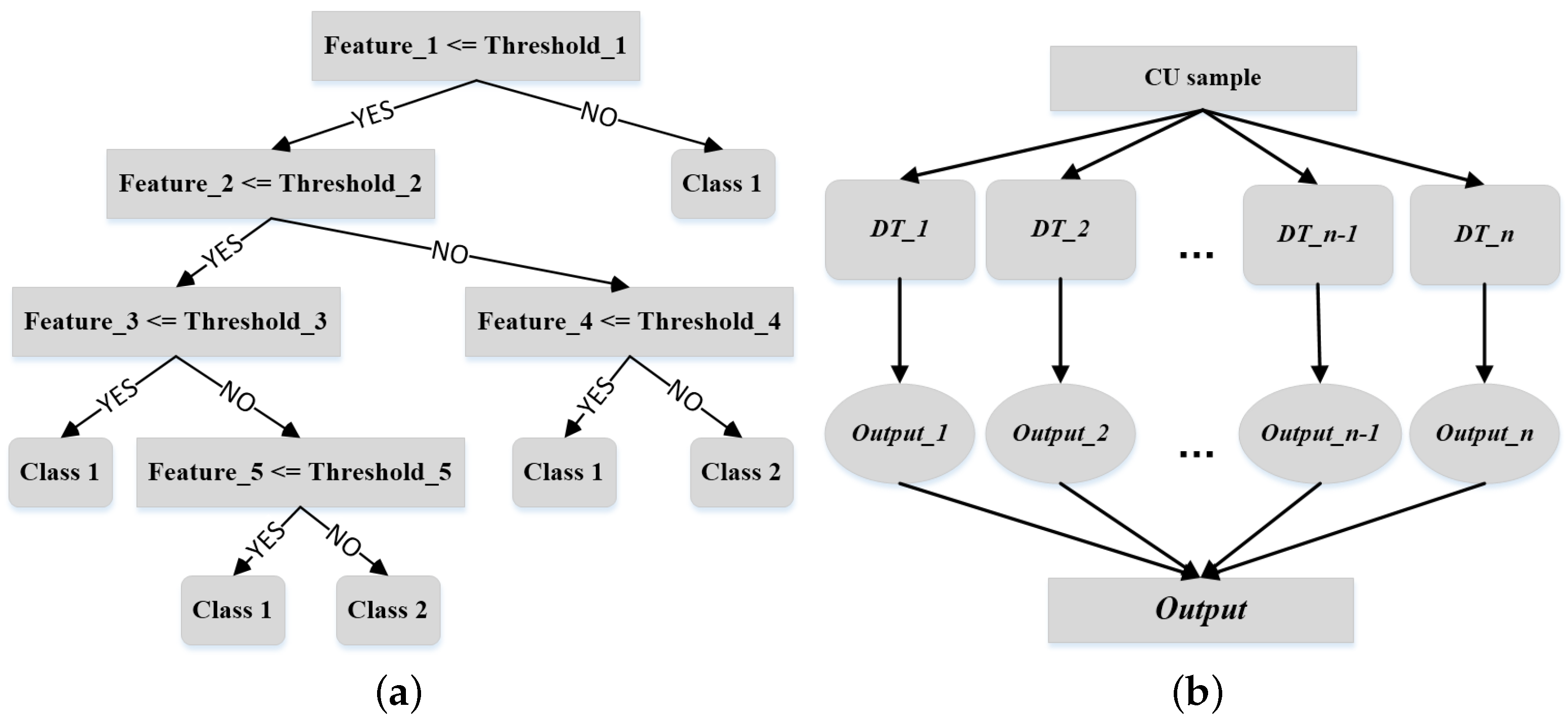
3. Fundamental Knowledge on Bagged Tree

Because our approach aims at exceeding the existing fast algorithms by using bagged tree model, a brief introduction of this machine learning technique is provided in this section.
Briefly, whether to split a CU or not is a binary problem. Many classifiers have been proposed to solve it. Decision tree [26] is one of the most widely used machine learning technologies. It represents a tree-like decision procedure for determining the class of a given instance. To illustrate this procedure, let us consider Figure 2a. Decision tree classifier completes a classification task by using a tree structure, in which each leaf node contains a class label and each father node contains a feature decision procedure (i.e., feature value and threshold) as well as a branch to another node. In Figure 2a, F e a t u r e _ n stands for the nth feature of a sample to be classified and T h r e s h o l d _ n stands for the corresponding threshold. According to this threshold, the classification process is completed. Besides, Class 1 and Class 2 are target classes that a sample belongs to.
Compared to other machine learning algorithms, decision tree has its own advantages. Firstly, decision tree is easier to understand and implement. Most importantly, the preparation of train data for decision tree is always simple while other models usually request data normalization such as deleting of the redundant or blank attributes. Especially, it can deal with large-scale data set in a short period of time and is not sensitive with missing values.
However, it is easy for decision tree model to be overfitting. Decision tree is quite sensitive to the specific data on which they are trained. If the training data is changed (e.g., a tree is trained on a subset of the training data), the resulting decision tree can be quite different leading to different decisions.
To address this problem, the bagged tree model is generated, in which advanced bagging techniques and decision tree techniques are combined. In the training phase, it creates many random sub-sets of training dataset generated with overlap. Then one decision tree model is trained by each sub-set. Finally, all the decision tree models are combined to form a bagged tree model. For prediction, the bagged tree model calculates and outputs the average of probabilities from each decision tree model, as is shown in Figure 2b. In Figure 2b, D T _ n is the nth decision tree classifier of all the classifiers that make up bagged tree model. O u t p u t _ n is the output of the nth decision classifier, and it is a value of probability that a sample will be classified to the target class. In this way, the output of a bagged tree model is calculated by using the following equation,
p = p 1 + p 2 + p 3 + + p N b a g s 1 + p N b a g s N b a g s
where N b a g s is the number of decision trees in the bagged tree model. Final output of model is calculated according to these N b a g s decision trees. p is the average probability of N b a g s decision trees and also is the output of the bagged tree model. Similarly, α is another key parameter for the bagged tree model. The size of trees in the bagged tree can be controlled through the parameter α . It influences the maximal percentage of training data in the leaves, so in some sense it is reverse to the size of the tree. The value of 1 produces a stump while the value of 0 represents a full tree. The following values of α can be used in the training, i.e., 1, 0.5, 0.2, 0.1, 0.05, 0.02, 0.01, 0.

4. Our Fast CU Partitioning Approach

As mentioned above, the CU partitioning procedure can be significantly accelerated by the prediction of classifiers through picking some critical features of the current under-processing coding unit. According to the probability output by the bagged tree classifier as well as the corresponding thresholds, the proposed fast CU partitioning method determines whether the current CU should be split or not. We describe the techniques used by our approach in following sections.

4.1. Framework of the Frame-Wise Beforehand Prediction

In HEVC intra-coding, the frames to be encoded are independent. Information from other frames is not required when current frame is being encoded. As a result, we can take a strategy of beforehand prediction so that the CU partitioning prediction has been completed when the encoder is encoding the last frame. Thus, a frame-wise prediction and encoding can be carried out without any feature extraction and prediction overhead. The framework of the proposed frame-wise beforehand prediction is shown in Figure 3. To the best of our knowledge, this parallel prediction strategy is proposed for the first time in CU size decision fast algorithms.
Specifically, in intra-coding scenario, the frame-wise beforehand prediction approach prefetches one frame and conducts feature analyses, in parallel with the currently coded frame. While it requires more computing resources, the extra computing resources needed by beforehand prediction is much less than that required by encoding an intra-frame. In this way, the complexity of feature extraction and prediction is reduced by using a little more computing resources.

4.2. Flowchart of the Proposed Bagged Tree Based Fast CU Size Determination Algorithm

Figure 4 shows the flowchart of the proposed fast CU size decision algorithm for video intra-coding. As we can see from Figure 4, the proposed method is a recursive process. When it comes to the process of a single CTU, the CTU will be regarded as a CU in depth 0. First, a judgement that if the number of samples collected for adaptive threshold determination is reached will be taken. The sample collection and threshold determination process will be described in details in Section 3. Once the threshold values are decided, the splitting probability of current CU will be extracted, and it will be fed to the label determination part as well as the thresholds of special depth. Then the probability will be transferred to the split flag (the split decision) of a CU. The values 0, 1 and 2 (the output of the split flag judgement structure in Figure 4) represent non-split, split and uncertain prediction which should check the true cost by RDO. If the split flag of a CU is 0, it will only check the cost of the CU in current depth, and the searching procedure will be terminated. In this way, time spent by RDO on next several depths can be saved. If the split flag of a CU is 1, the cost check of current depth will be skipped and go straight into the next depth. Respectively, the time spent on finding optimal cost in current depth will be saved. Due to the misclassification, there will be a number of samples predicted to uncorrected class. Aiming at reducing the computational complexity in CU size decision while maintaining the RD performance, we implement full RDO to CUs classified to class 2 so that we can get a precise RD cost. Note that the proposed algorithm for depth i is a recursive process. This fast CU size decision will be executed until it reaches the maximal depth 3. In other words, CUs of sizes 64 × 64, 32 × 32, 16 × 16 will be predicted by the proposed model. The minimal CUs of size 8 × 8 are processed by RDO automatically. The proposed algorithm only focuses on CU instead of PU.
In addition, the bagged tree model is trained offline in this proposed method. Because we not only will not gain the complexity burden of the encoder, i.e., the training time spent overhead will not be put to the encoder, but also can select high quality training samples to form our train dataset. We collect various samples, for example, the samples in different resolution, different depth and various scenes. As a result, we design different classifiers for different Quantization Parameters (QPs) and resolutions. In other words, for each combination of QP (22, 27, 32, 37) and resolution class (A, B, C, D, E), we generate an independent bagged tree model. So there are 20 models in total. Compared with existing methods that employ one machine learning model for each CU size (64 × 64, 32 × 32, 16 × 16), our method is unique and simpler.

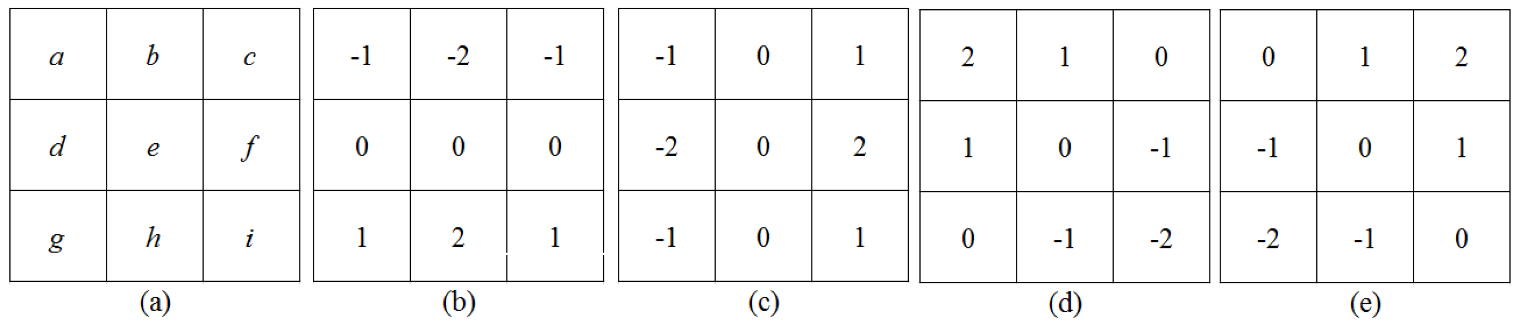
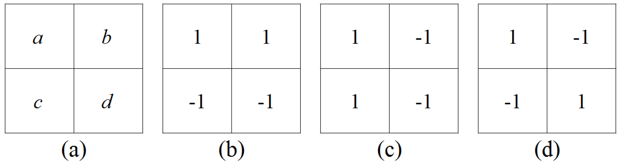
4.3. Feature Analysis And Extraction

Statistically, we have some prior knowledge for CU size decision. For instance, homogeneous regions are more likely to be encoded in larger CUs. Regions with same attributes but in different resolution sequences will be processed to different results. Larger CUs are more likely to be further partitioned than smaller CUs, which shows depth information effects. With such observations, we can derive a number of features. Moreover, to find out those most effective features, we first employ features, which are commonly used in other works [9,27,28]. Then we extend the number of features candidates to 32 totally. These features from different domains, i.e., spatial information, statistical data, pre-encoding data and encoding parameters, are listed in Table 1. We will describe these feature candidates in details as follows.
For features related with spatial information, we extract 8 feature candidates, i.e., from No. 4 to No. 11 as shown in Table 1. For CU to be determined, we extract RD cost and average depth of its neighboring CTUs (above, left, above left and above right). These values are presented as m _ n b C t u A b o R d and m _ n b C t u A b o D e p t h , etc.
Besides, we also calculate some statistical data as our feature candidates. In Table 1, No. 1, No. 2 and the candidates from No. 18 to No. 29 are all statistical data. To analyze the relationship between splitting result and block flatness, we calculate its corresponding mean value and variance value. They are No. 28 and No. 29 in Table 1. HEVC adopts a quad-tree based CU partitioning structure, so the difference between the single CU and it’s four sub-CUs will make an effort to the partitioning decision. We use the variance of the mean of sub-CUs to measure the texture of current CU. Specifically, we calculate four means of four sub-CUs, then derive the variance of these four means according to the following equations.
m e a n S u b = 1 n i = 0 n 1 p i
m _ m e a n M a i n = 1 4 i = 0 3 m e a n S u b i
m _ var M e a n S u b = 1 4 i = 0 3 m e a n S u b i m _ m e a n M a i n 2
m _ var M a i n = 1 n i = 0 n 1 p i m _ m e a n M a i n 2
where p i is the luminance value of the ith pixel. m e a n S u b is the mean of pixels among a sub-CU. Moreover, m _ m e a n M a i n is the whole pixels mean of four sub-CUs.
Used by many works [9,27,28], the variance of the variances of four sub-CUs, i.e., m _ v a r V a r S u b , also can reflect the correlation among these four sub-CUs. m _ v a r V a r S u b is calculated according to the following equations.
varSub = 1 n i = 0 n 1 p i m e a n S u b 2
m e a n V a r S u b = 1 4 i = 0 3 varSu b i
m _ varVarSub = 1 4 i = 0 3 varSu b i m e a n V a r S u b 2
For m _ e d g e S o b e l , it is a result of edges detection by using the Sobel operator. Two traditional Sobel filters (i.e., horizontal and vertical) are employed, which are shown in Figure 5b,c. They are applied on each block of size 3 × 3 with overlap in current CU, as shown in Figure 5a. Furthermore, we extend the Sobel filters with two more directions (i.e., 45 ° and 135 ° ), which are Figure 5d,e. m _ e d g e S o b e l is calculated by the following equations.
g h = a 2 b c + g + 2 h + i
g v = a 2 d g + c + 2 f + i
g 45 = 2 a + b + d f h 2 i
g 135 = b + 2 c d + f 2 g h
m _ e d g e S o b e l = 1 N 2 2 k = 0 N 2 2 g h k 2 + g v k 2 1 / 2
where N is the size of current CU (64, 32 or 16), and k is the kth block of size 3 × 3 in current CU.
We also reuse the features proposed by other works [9], for instance, m _ n m s e as well as m _ d c o m . They are calculated as follows:
p ¯ i , j = 1 8 p i 1 , j 1 + p i 1 , j + p i 1 , j + 1 + p i , j 1 + p i , j + 1 + p i + 1 , j 1 + p i + 1 , j + p i + 1 , j + 1
m _ n m s e = 1 N 2 i = 0 N 1 j = 0 N 1 p i , j p ¯ i , j 2
m _ d c o m = 1 N 2 2 k = 0 N 2 2 g h k + g v k + g 45 k + g 135 k
where p i , j is the luminance pixel value at location ( i , j ) in current CU, and k is the same as above.
To some degree, the splitting result may be also in connection with the number of interest points within current CU. As a result, we calculate the number of interest points with the method of interest point detection mentioned in [29]. Feature m _ n u m A v e I n t e r e s t P o i n t represents the average number of interest points for each pixel among a CU. It reflects how much attention people would pay to a CU and how many details a CU contains. The three filters in Figure 6 are used on each pixel among current CU, and three corresponding results D x x , D y y , D x y are obtained as filter responses in the horizontal, vertical, and diagonal directions, respectively. We use Equations (17)–(19) to obtain the final value of feature m _ n u m A v e I n t e r e s t P o i n t for current CU. Equations (17)–(19) are as follows:
P i , j = D x x D y y 0.9 D x y 2
B i , j = 0 , P i , j < t 1 , P i , j t
m _ numAveInterestPoint = 1 N 2 i = 0 N 1 j = 0 N 1 B i , j
where P(i, j) is the interest value of pixel located at ( i , j ) . B(i, j) is the boolean value of being decided to be an interest point for pixel ( i , j ) . Moreover, t is the threshold for judging interest point. N is the size of current CU, 64, 32 or 16. Because the original interest points detection method uses more complicated filters to obtain P(i, j), which is time consuming, the relative weight 0.9 is used to minimize the errors between them.
Authors in [29] also proved that Haar wavelet convolution can reflect the texture information more precisely. As for features extracted from Haar wavelet, because the traditional Haar wavelet transform only processes information along the horizontal and vertical directions, we extend it with diagonal direction. These three Haar filters of different directions are shown in Figure 7b–d. Figure 7a is an example of pixel values for a 2 × 2 pixel block. For example, the response of the horizontal filter on a 2 × 2 pixel block is calculated as follows:
d x = a + b c d
For a target CU, it is split up regularly into 2 × 2 non-overlapped sub-squares. Then we perform Haar wavelet on each 2 × 2 square to generate its corresponding responses on three different directions (i.e., d x , d y and d x y ) using the filters in Figure 7b–d. Take m _ h a a r S u m x and m _ h a a r S u m A b s x for examples, they are calculated by:
m _ h a a r S u m x = 1 N 2 2 k = 0 N 2 2 1 d x k
m _ h a a r S u m A b s x = 1 N 2 2 k = 0 N 2 2 1 d x k
where N is the size of current CU (64, 32 or 16), and k is the kth non-overlapped block of size 2 × 2 in current CU. d x k represents the value d x of the kth sub-square.
Furthermore, we pre-encode the current CU with PLANAR mode, so that we extract 7 features based on pre-encoding results. As is shown in Table 1, m _ a v e C B F is the Coded Block Flag(CBF) of current CU encoded with PLANAR mode. Besides, t o t a l C o s t , t o t a l D i s t o r t i o n and t o t a l B i n s are the cost, distortion and number of bits, respectively. Moreover, m _ c o s t H a d a m a r d , m _ s a d H a d a m a r d , m _ b i t s H a d a m a r d are the Hadamard encoding related cost, square absolute difference, number of bits, respectively.
We design their classifiers for each QP (22, 27, 32, 37) as well as each resolution class (A, B, C, D, E) instead of on the depth level. Considering the influence of CU depth, we introduce depth related feature candidates, which are represented as d e p t h C l a s s 1 , d e p t h C l a s s 2 and d e p t h C l a s s 3 in Table 1.
To measure the contributions of these feature candidates, our bagged tree based approach can automatically rank features during training phase. The ranking results are generated according to the importance score of each attribute. The importance score of a feature in a bagged tree model is calculated by averaging all the importance scores in individual decision tree models. Moreover, it is in the range of 0 to 1. The importance score of an attribute in a single decision tree model is calculated according to how many times this feature is used on each node to generate a tree. Specific methodology on how to generate the importance scores is presented in [30].
Figure 8 shows the importance value of each feature for different bagged tree models. It is obvious that several features with high importance value distribute intensively around Nos. 2, 3, 8, 9, 19, 21 and No. 25–No. 30. It proves that numbers of features among 32 feature candidates are not necessary. While there are common features existing among the top several features for each model, the number of common features is not big enough. Hence we can not achieve a satisfactory result according to these common features. As a result, it is necessary to select different features for each classifier to achieve the best results, and this is also the motivation of designing one classifier for video sequences in the same resolution and QP value.
As we all know, the more features we use to train a model, the more precise results we can get, while the time spent on feature extraction increases. So we can make a tradeoff between accuracy and time saving by controlling the number of active features. Observing from Figure 8, we conclude that the importance value keeps in a relatively high level for the top 10 features in each classifier. The importance value of other features remains small, which means they will not make much contribution to a better result but increasing time overhead. As a result, we pick top 10 key features as the final feature set for each classifier.

4.4. Training Data Generation

In order to collect representative samples and generate a training set of high diversity, we select five sequences from the standard test set. They are PeopleOnStreet (Class A 2560 × 1600), Cactus (Class B 1920 × 1080), BasketballDrill (Class C 832 × 480), RaceHorses (Class D 416 × 240) and Johnny (Class E 1280 × 720), respectively. Each of these sequences is encoded under four QPs (22, 27, 32, 37). In this way, the features and the corresponding ground truth of split flag are collected. To balance the samples of different depths and labels, we randomly select 6000 samples, whose label is split, from depth 0. Then we also select 6000 samples labelled non-split for depth 0. In case, the total number of samples of the specified label can not reach the number of samples we want to extract, for example there are only n (n is smaller than 6000) samples labelled non-split, and all the n samples will be extracted. Then, to balance the samples of different labels, we also extract n samples whose label is split. In this way, 12,000 samples (this number will be smaller, if the number of samples in a class is smaller than 6000) are extracted for each depth. The samples from depth 1 and depth 2 are generated in the same way. So we can generate a dataset consisting of 36,000 samples for one bagged tree model. As a result, there are 20 data sets in total, each of which is for a model of a certain QP and resolution class.

4.5. Bagged Tree Design

After getting the splitting probability of a CU, we can decide that if current CU should be split or not. Traditional bagged tree classifier usually generates the final predicted labels by implying one threshold on the output probability. In this way, it will generate a classification edge between two classes as shown in Figure 9a. Setting the threshold as 0.5, we calculate the prediction accuracy of different depths on our datasets. Statistical results are shown in Table 2. It can be observed from Table 2 that the average accuracy of the traditional bagged tree model for depth 0 is 92.65%, and it’s 85.05% and 79.40% for depth 1 and 2, respectively.
To improve the prediction accuracy, we model the CU partitioning process as a three-class classification problem through using the probability output by the bagged tree and the thresholds we set. Instead of using two classifiers to complete this task, we only imply one bagged tree model with two threshold to achieve this. Hence we can enhance the prediction accuracy as well as simplifying the complexity.
Figure 9b shows the example classification edges of the three-output classifier proposed by us. In Figure 9, Class 0 represents non-split and class 1 stands for split. As for other samples which are predicted to neither class 0 nor class 1, we put them into class 2, which are going to be processed with RDO. By controlling the classification edges, we can tell the precision of class 0 and class 1 is improved, and the encoding performance also improves.
Obviously, two corresponding thresholds are needed to generate two edges in Figure 9b. In the proposed approach, the edge between class 0 and class 2 is generated by comparing a low threshold (represented as T L ) and a possibility output by bagged tree model. Similarly, we generate the edge that divides class 1 and class 2 by comparing the possibility with a high threshold (as known as T H ). In this way, the final label of a CU is decided. Equation (23) shows how to label a CU according to the related probability and thresholds, it is shown as follows:
s p l i t F l a g = 0 ( n o n s p l i t ) , p < T L 1 ( s p l i t ) , p T H 2 ( R D O ) , o t h e r w i s e
where s p l i t F l a g is used to represent the predicted labels of a CU.
As described in Section 3, different actions are carried out for CUs which are predicted to different classes. However, RDO is time consuming so that the more the samples of class 2 have, the more time the encoding process takes. Obviously, we can control encoding time and accuracy by controlling the two classification edges of a classifier. If we increase T H , the number of samples predicted to class 1 decreases while the number of samples predicted to class 2 increases. Similarly, if we decrease T L , less samples are predicted to class 0 but more samples are predicted to class 2. Moreover, in any condition of these two cases, the encoding performance both improves, because more correct predictions are generated in whichever case.

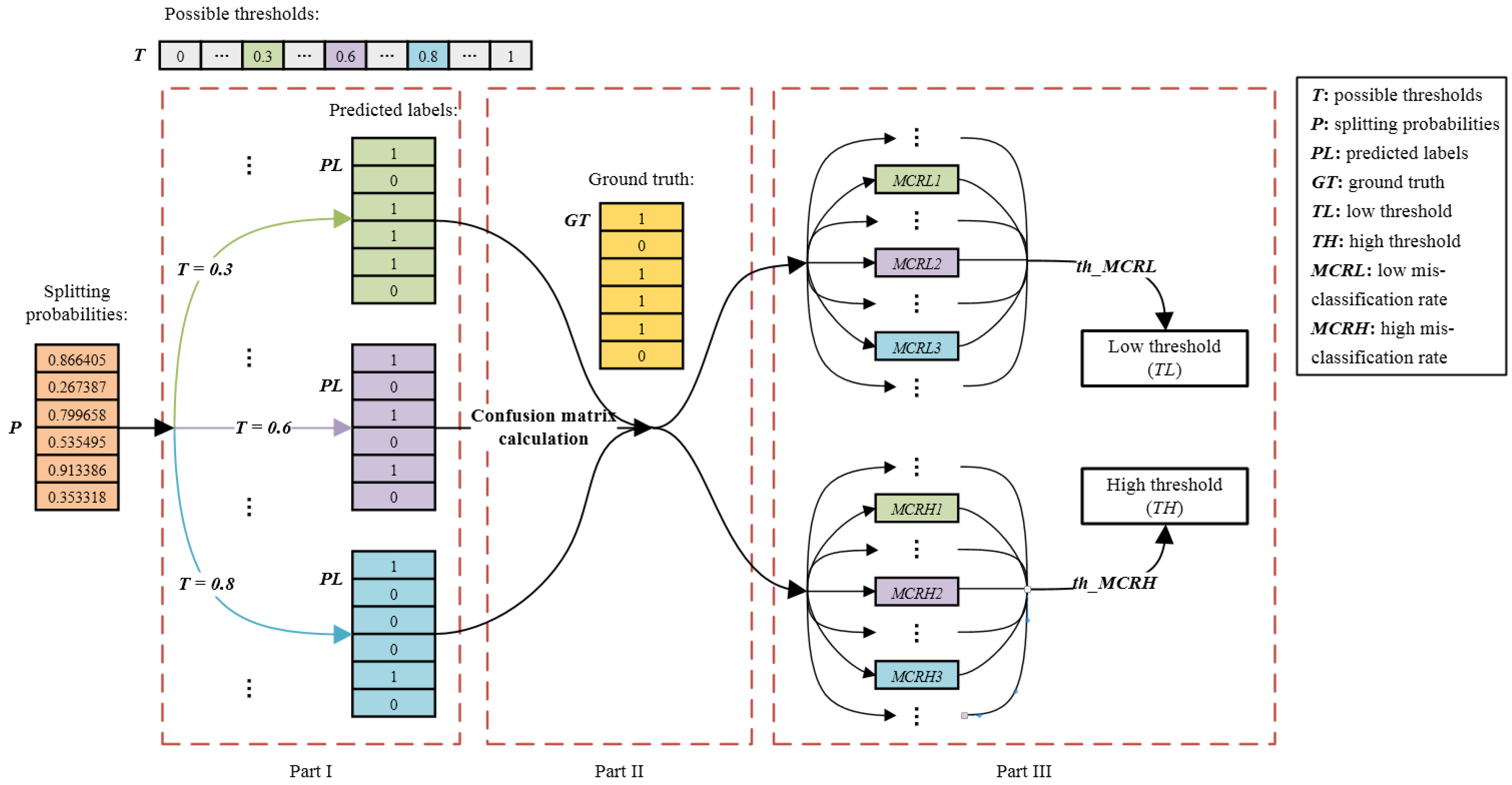
4.6. Adaptive Threshold Determination

In this paper, we apply only one bagged tree model on video sequences that are in the same resolution and QP value. Because false predictions at different CU depths will lead to a different increase of BD-rate loss as well as encoding time, we can not implement the same T H and T L on CUs in different depths, even in the same sequences. Thus, for CUs from the same sequence but in different depths, a classifier must have the corresponding individual thresholds. Moreover, we denote T L and T H for depth 0 as T L 0 and T H 0 , similarly, T L 1 and T H 1 for depth 1, T L 2 and T H 2 for depth 2.
Table 3 shows the confusion matrix of the proposed bagged tree classifier. Because RDO performed on CUs in class 2 doesn’t bring BD-rate loss, only class 0 and class 1 are considered. In Table 3, T N is the number of CUs that are correctly classified as Class 0. F P is the number of CUs that are falsely classified as Class 1. Similarly, F N and T P are the number of CUs whose ground truth is class 1, while they are falsely classified and correctly classified, respectively. We can derive that the number of CUs labeled as Class 0 is T N + F P , and the number of CUs, whose true labels are 1, is F N + T P . According to numerous of experiments, we find that F P decreases as T L decreases in each depth. Besides, F N decreases as we increase T H . As expected, we can improve the accuracy by adjusting T H and T L for each depth. However, we achieve less time saving, because we carry out full RDO for these CUs whose splitting probability is between T L and T H . As a result, the more CUs classified to class 2 are, the more RDO process is carried out.
To maintain sufficient prediction accuracy, we propose an adaptive threshold determination method to calculate these six thresholds ( T L 0 , T H 0 , T L 1 , T H 1 , T L 2 and T H 2 ) for each video sequence to be encoded. In this method we adaptively calculate T L and T H of each depth by using negative misclassification rate (denoted as M C R L ) and positive misclassification rate (denoted as M C R H ). M C R L and M C R H can be calculated according to the following equations.
M C R L = F N F N + T P
M C R H = F P T N + F P
Obviously, T H and T L for each CU depth must be calculated before activating the proposed fast CU splitting approach in video encoding process. We first use RDO to encode the first 256 CTUs of a video sequence, which contains 1024 CUs of depth 1 as well as 4096 CUs of depth 2, and the splitting probabilities are calculated by our bagged tree model in the mean time. In this way, the splitting probabilities and the corresponding ground truths for CUs in the same depth are collected as the samples. They are denoted as P and G T in Figure 10. Figure 10 shows that how T L and T H for a certain depth are calculated from these samples.
Using a threshold, we can transfer the splitting possibility calculated by the bagged tree model to a CU’s predicted label, and it is illustrated in Part I of Figure 10. Generally, there will be a number of samples predicted falsely, and so the confusion matrix is generated. First, we go through all the possible thresholds (denoted as T) from 0 to 1 with step 0.0005, i.e., 0, 0.0005, 0.001, …, 0.9990, 0.9995, 1, and calculate the corresponding M C R L and M C R H (shown as M C R L 1 , M C R L 2 , M C R H 1 , M C R H 2 and so on in Figure 10). The calculation process is shown in Part II of Figure 10. Then according to the preset thresholds t h _ M C R L and t h _ M C R H , we pick the highest probability whose M C R L is smaller than t h _ M C R L as the final low threshold T L . Similarly, the lowest probability whose M C R H is smaller than t h _ M C R H is chosen as the final high threshold T H . In this way, the encoder can adaptively calculate T L and T H of each depth for every video sequence only by using of two parameters t h _ M C R L and t h _ M C R H . The adaptive thresholds determination process is shown in Part III of Figure 10, and its mathematical expression is shown as following equations.
T L = max T s . t . M C R L t h _ M C R L
T H = min T s . t . M C R H t h _ M C R H
For CUs in depth 1 and 2, we will execute this process so that we get 4 thresholds in total ( T H 1 and T L 1 for depth 1, T H 2 and T L 2 for depth 2). According to Table 2, we do not imply the adaptive threshold determination process for depth 0, because the accuracy of depth 0 is high enough and the additional process will not bring too much improvement. As a result, T H and T L for depth 0 (i.e. T H 0 , T L 0 ) are set to 0.5 directly.
In summary, the encoder can adaptively decide T H and T L for depth 1 and 2 by processing the data collected from the samples encoded before the start of the proposed approach. We only need to set two misclassification rates t h _ M C R L and t h _ M C R H , which work for both depth 1 and 2. However, their value settings need sufficient experience.

5. ABTFA

For BTFA, an adaptive thresholds determination algorithm is proposed to calculate T L 1 , T H 1 , T L 2 and T H 2 according to the coding results of several beginning frames of current video sequence. However, in some cases including fast motion, the thresholds calculated according to the several beginning frames may not suit for the whole video sequence. Besides, a proper thresholds setting requires many experiences to achieve a certain BD-rate loss or a target time saving. To address this problem, we upgrade BTFA to the advanced bagged tree based fast algorithm (ABTFA), with which more general thresholds are calculated according to the analysis of training sequences. Furthermore, using ABTFA, we can calculate optimal thresholds satisfying a certain constraint, i.e., a target BD-rate loss or a target time saving.
First, we use the encoder, in which the bagged tree based fast algorithm without adaptive thresholds determination algorithm is implied, to encode the five sequences in training set. As for the thresholds T L 1 , T H 1 , T L 2 , T H 2 , their values are picked from their domain with step 0.1. Specifically, T L 1 and T L 2 are set to be 0, 0.1, 0.2, 0.3, 0.4, 0.5 one by one, while T H 1 and T H 2 are set to be 0.5, 0.6, 0.7, 0.8, 0.9, 1. In this way, we obtain 6 × 6 × 6 × 6 = 1296 thresholds combinations, and the videos in the training set are encoded with each of these combinations. Finally, 1296 pairs of BD-rate loss and time saving are generated under the corresponding thresholds. The 3-D surface in Figure 11 shows the relationship among them. For the purpose of visualization, only BD-rate loss and time saving with respect to T L 1 , T H 1 as well as T L 2 , T H 2 are shown in Figure 11, because we can not visualize the surface of a 5-D space.
According to the experiments on the training sequences, the exact mathematical relationship among the BD-rate loss and four variables ( T L 1 , T H 1 , T L 2 , T H 2 ), as well as that of time saving and these four variables can be explored. In Equation (28), f ( x ) is used to represent the function between BD-rate loss and T L 1 , T H 1 , T L 2 , T H 2 . Similarly, the function g ( x ) represents the relation between time saving and T L 1 , T H 1 , T L 2 , T H 2 . Function f ( x ) and g ( x ) are shown as follows.
b i t r a t e L o s s = f ( x ) = f T L 1 , T H 1 , T L 2 , T H 2
t i m e S a v i n g = g ( x ) = g ( T L 1 , T H 1 , T L 2 , T H 2 )
Due to the nonlinear relation of these variables, we use neural network to fit these data points generated from massive experiments. The structure of the neural network used by us is shown in Figure 12. Only two layers are implied and the number of neurons in hidden layer is set to be 10. Given consistent data and enough neurons in its hidden layer, a two-layer feed-forward network with Sigmoid hidden neurons and linear output neurons (fitnet), can fit multi-dimensional mapping problems arbitrarily well. The network will be trained with Levenberg-Marquardt backpropagation algorithm (trainlm), unless there is not enough memory, in which case the scaled conjugate gradient backpropagation (trainscg) will be used. As a result, we generate two mathematic modules after the neural network training. One module is f ( x ) and the other is g ( x ) .
As we can see from Figure 11, BD-rate loss (the less the better) increases with the increment of time saving (the more the better). In real applications, there usually is an exact constraint of BD-rate loss or time saving, which can not be achieved by setting thresholds roughly. On the one hand, for a given upper bound of BD-rate loss, we want to maximize the time saving. On the other hand, we also want to minimize the BD-rate loss for a given lower bound of time saving. They can be modeled as the following optimization problem.
T L 1 , T H 1 , T L 2 , T H 2 = arg max T L 1 , T H 1 , T L 2 , T H 2 g ( x ) s . t . f ( x ) < B L t a r
T L 1 , T H 1 , T L 2 , T H 2 = arg min T L 1 , T H 1 , T L 2 , T H 2 f ( x ) s . t . g ( x ) > T S t a r
where B L t a r is the target BD-rate loss, i.e., the upper bound of BD-rate loss and T S t a r is the target time saving which should be achieved.
To calculate the optimal thresholds T L 1 , T H 1 , T L 2 , T H 2 , which satisfy the conditions above, the Matlab function f m i n c o n ( ) is used to solve the above optimization problems. As a result, once given a target BD-rate loss or time saving, the optimal thresholds can always be found to meet the constraints. Thus, using ABTFA, we can not only maximize the time saving according to a constraint of BD-rate loss exactly, but also can minimize the BD-rate loss according to a given time saving constraint.

6. Experiments

To verify this proposed fast CU splitting algorithms BTFA and ABTFA, we implement them on the reference HEVC platform HM16.7. In our experiments, the sequences of HEVC standard test sets, whose resolutions are 2560 × 1600 (Class A), 1920 × 1080 (Class B), 832 × 480 (Class C), 416 × 240 (Class D), 1280 × 720 (Class E), are encoded to verify the performance. Coding parameters such as number of frames to be encoded are set as default [31]. Besides, all-intra-main configuration is adopted and all the frames are encoded as intra-frames. The bit distortion rate (denoted as B D - r a t e ) is employed to evaluate the coding performance of the proposed method. Simulations are executed on a windows 10 64-bit operating system workstation with Intel(R) Xeon(R) CPU E5-2623 v3 @ 3.00 GHz and 3.00 GHz (2 processors), 64.0 GB. Experiments are taken under QPs 22, 27, 32, 37, respectively. Besides, the time saving ratio denoted by T S is used to measure complexity reduction of encoding methods. It is defined as
T S = t i m e o r i t i m e p r o t i m e o r i × 100 %
where t i m e o r i denotes the time spent by the original HM16.7 encoder. Moreover, t i m e p r o is the time spent by the encoder on which the fast algorithm is implemented.
We use α and N b a g s to control the size and the number of the trees, respectively. α is set as 0.01, 0.01, 0.01, 0.01, N b a g s is set to be 50 for QP values 22, 27, 32, 37. As for the adative threshold determination in BTFA, it is only implied on depths 1 and 2, and T H _ M C R L , T H _ M C R H are set separately for the corresponding depths 1, 2. T H and T L for depth 0 are both set to be 0.5.

6.1. Experiment Results Of BTFA

Table 4 shows the BD-rate loss and the time saving achieved at each test sequence encoded by the encoder on which BTFA is implemented. Different combinations of the values for M C R L 1 , M C R H 1 , M C R L 2 and M C R H 2 are set for comparison. Specifically in Table 4, five groups of their values are tested. Respectively, they are [0.02, 0.03, 0.02, 0.03] as group one (G1), [0.07, 0.03, 0.07, 0.03] as group two (G2), [0.02, 0.08, 0.02, 0.08] as group three (G3), [0.07, 0.08, 0.02, 0.08] as group four (G4) and [0.02, 0.08, 0.07, 0.08] for group five (G5). Besides, for the value set of [0.05, 0.05, 0.05, 0.05] (namely group 6 denoted as G6), its result is discussed in Section 6.3. The thresholds of misclassification rates (i.e., M C R L 1 , M C R H 1 , M C R L 2 and M C R H 2 ) influence the rate distortion and the complexity reduction. Results in Table 4 confirm the influence. As we can see, with the general increase of thresholds for misclassification rate, BD-rate loss and time saving increase proportionally.
Compared to the results of G1, G2 achieves more time saving with the sacrifice of little BD-rate loss. Moreover, the difference of thresholds is only 0.05 increase of M C R L 1 and M C R L 2 . Furthermore, when we increase 0.05 to the values of M C R H 1 and M C R H 2 in G1 (so G3 is generated), similar increments of BD-rate loss and time saving occur. However, when having a close-up view of the performance change of G2 and that of G3, we observe that the time saving of G2 increases more. It shows that the same change of the values for low misclassification rate thresholds takes more effect on time saving than that for high misclassification rate thresholds. Because once a CU is predicted to be nonsplit, the encoding check of all its corresponding sub-CUs will be skipped. As a result, the misclassification of class 0 influences the encoding time wider than that of class 1.
Compared with G3, the value of M C R L 1 for G4 is increased by 0.05. As a result, the BD-rate loss and the time saving of G4 both increase. Similarly, only the value of M C R L 2 in G5 is increased by 0.05 compared to that in G3. However, the BD-rate loss under G4 is higher than that under G5, and the time saving also changes more. It means that the influence brought by the change of misclassification rate thresholds for depth 1 is greater than that for depth 2. This is because sub-CUs under a CU of depth 1 outnumbers sub-CUs under a CU of depth 2, and the effect of changing M C R L 1 and M C R H 1 is bigger than that of changing M C R L 2 and M C R H 2 . It reminds that smaller values of M C R L 1 and M C R H 1 should be prioritized when possible.

6.2. Experiment Results Of ABTFA

With ABTFA, we can calculate proper thresholds of T L 1 , T H 1 , T L 2 and T H 2 under a given target BD-rate loss or time saving according to Equations (30) and (31). To verify the feasibility and the accuracy of ABTFA, rate-distortion and encoding time under different constrains are shown in Table 5. As we can see, when B L t a r is set to be 0.6%, the results of BD-rate loss vary from 0.06% to 1.67%, and the average value of BD-rate loss is 0.68%, which is 0.08% higher than B L t a r . To achieve a higher encoding time reduction with a sacrifice of bit-rate, B L t a r is set to be 0.9%, which is shown in the last two columns of Table 6. The difference between BD-rate loss results and B L t a r is as low as 0.06%. Meanwhile, the encoder achieves a satisfactory value as high as 47.87%. Besides, when the value of T S t a r is set to be 45% and 50% as shown in Table 5, the encoding time is reduced by 46.15% and 57.11% while the BD-rate loss is 1.27% and 2.45%, respectively. While there is still some bias between encoding results and target constrains, the errors in terms no matter of BD-rate loss or time saving are both acceptable. Obviously, the samples used to generate regression models (i.e., f ( x ) and g ( x ) ) can not reflect the relations in all video sequences, so we can only achieve the results around the target value rather than precise ones. In short, experimental results show that the proposed ABTFA works well on calculation thresholds for each depth according to a certain constraint. This also means that the encoder can achieve the results according to the people’s requirement without requests of additional thresholds setting experience.

6.3. Comparison with State-of-the-Art

To testify the coding effectiveness of the proposed fast CU size decision algorithms, we select five state-of-the-art algorithms including one algorithm DDET [32] based on traditional analysis, and three machine learning algorithms, FADT [33], FARF [34] and DA-SVM [17], for the comparison of performance. Specifically for machine learning methods employed in these three algorithms, FADT uses decision tree, FARF is based on random forest, and DA-SVM uses SVM. As one knows, the key technique of random forest and bagged tree is both decision tree, so the comparison is very meaningful.
Table 6 presents BD-rate loss and time saving among DDET, FADT, FARF, DA-SVM and the proposed BTFA and ABTFA. In Table 6, the thresholds for misclassification rate are the same as those in group 6 (G6), i.e., [0.05, 0.05, 0.05, 0.05]. Moreover, the result of ABTFA is under a constraint for BD-rate loss which is 0.9%.
It is observed that DDET achieves a BD-rate loss from 0.36% to 1.86%, and 0.95% on average. Though the BD-rate loss is similar with that of ABTFA, the time saving is only 39.59%, which is 8.28% less than the 47.87% of ABTFA. Even compared with BTFA, DDET still does not have advantages in terms of both BD-rate loss and time saving. Its time saving can not exceed that of BTFA, moreover, the BD-rate loss of BTFA is 0.03% less.
As a fast approach based on decision tree, FADT scheme is quite a good competitor. Moreover, it achieves an average BD-rate loss of 1.15% as well as a time saving of 37.87%. However, no matter of the BD-rate performance or the time saving performance of FADT are worse than those of BTFA and ABTFA. Results show that the proposed bagged tree based approach exceeds the traditional decision tree based approaches.
Based on decision tree techniques, FARF uses random forest to improve the model performance. As a result, FARF achieves 1.30% BD-rate loss on average and saves as high as 52.30% encoding time, and it is very competitive. The complexity reduction of FARAF is 10.4% higher than that of BTFA while the BD-rate loss is about 0.38% more. Generally speaking, FARF and BTFA are equally matched. However, compared to ABTFA, FARF is only 4.43% higher in terms of time saving, while the BD-rate loss of FARF increases by as much as 0.34%. Obviously, the general performance of the proposed ABTFA approach is a little better than that of FARF.
According to related works [9,16,17], we can find that SVM based approaches are extensively researched and well performed. As we can see from Table 6, DA-SVM saves on average 47.6% encoding time than the original HM16.7. The time saving of DA-SVM is quite similar with that of the ABTFA, however the BD-rate loss of ABTFA is 0.42% less. It means the proposed ABTFA outperforms DA-SVM in terms of BD-rate loss, when maintaining the encoding time. Actually, if we set the bit-rate constraint of ABTFA as 1.38%, the time saving achieved by ABTFA is higher than the 47.6% of DA-SVM.
For the comparison between BTFA and ABTFA, we can observe that ABTFA gains about 5.78% time saving while the difference of BD-rate loss is negligible. This is because more advanced deep learning technique is applied to find the optimal thresholds for depths 1 and 2 under a target constraint.
To further demonstrate the performance of our proposed algorithm, we compare it with three additional algorithms on five video sequences. These three algorithms are all proposed most recently, and they are Huang’s algorithm [5], Liu’s algorithm [9] and Fu’s algorithm [25]. The BD-rate loss and the encoding complexity reduction are shown in Table 7.
From Table 7, we can find that the complexity reduction of the ABTFA is 2.83% and 0.66% more than that of Liu’s algorithm and Fu’s algorithm, respectively, while the BD-rate loss is 0.07% and 0.20% larger. We can conclude that their overall performances are about the same. Compared with Huang’s algorithm, the ABTFA does not have obvious advantage. However, there are various versions of the proposed algorithm, according to which we can make a tradeoff between the BD-rate loss and the complexity reduction. From Table 7, we can observe that the proposed BTFA-G1 outperforms all these three competitors with a huge advantage in terms of BD-rate loss, while its complexity reduction is slightly less. Specifically, the BD-rate loss of the BTFA-G1 is about half smaller than that of Huang’s algorithm, while the time saving is less by 19.03% which is acceptable considering the difference on BD-rate loss. While the time saving of BTFA-G1 is less than both Liu’s and Fu’s algorithms, the BD-rate loss is as much as 0.58% and 0.45% less, respectively. Generally speaking, the proposed algorithm is very flexible and can be applied according to various conditions. Our algorithm outperforms Huang’s, Liu’s and Fu’s algorithms by using different configurations (i.e., different versions of the proposed algorithm).

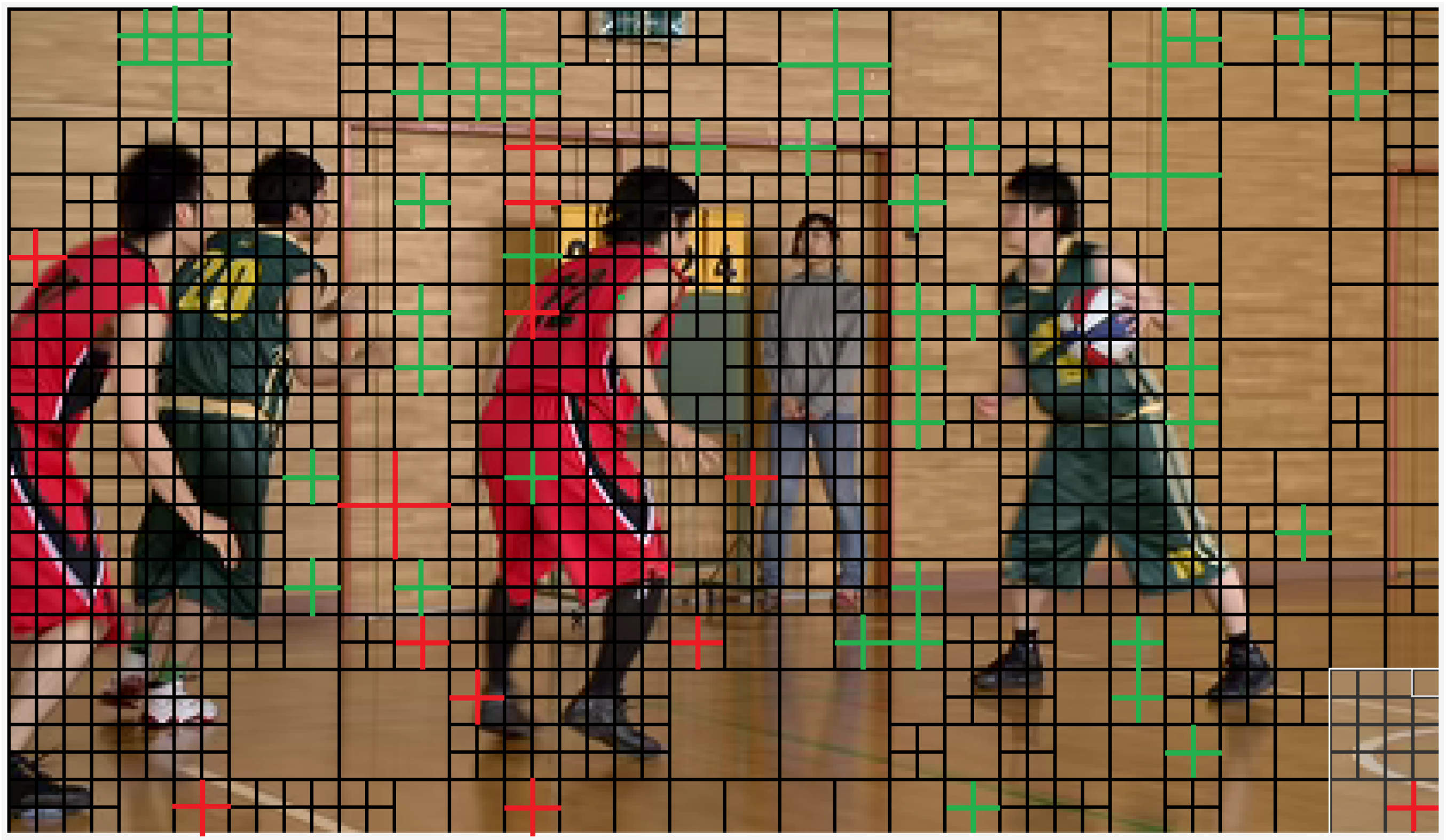
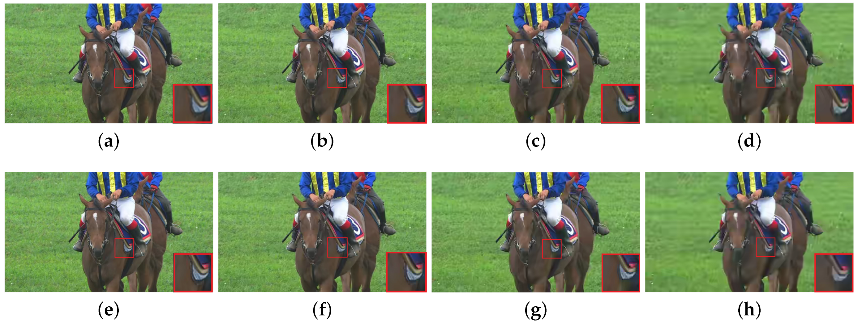
6.4. CU Partition Result Comparison between ABTFA and the Original HM16.7

To compare the decisions taken by the proposed ABTFA and the original HM16.7, we illustrate their partition decisions for the same frame. First, the 200th frame of sequence BasketballPass is encoded with original HM16.7 under QP 22, as a result, the partition results are shown in Figure 13. Black line in Figure 13 represents CU boundaries. Then, the same frame is encoded by HM16.7, in which the proposed ABTFA with BD-rate loss constraint 0.9% is applied. Figure 14 shows the CU boundaries decided by ABTFA. In Figure 14, black line represents the same partition decisions as those in Figure 13. Green line represents boundaries of CUs, which are split by original HM16.7 but are not split by ABTFA. On the contrary, red lines represents boundaries of CUs decided to be split by ABTFA but non-split by original HM16.7.
As we can see, the decoded two frames are almost of the same image quality. Compared with the partition results generated by original HM16.7, ABTFA maintains much correctness of partition decisions (i.e., black line in Figure 14). However, there are still some differences (i.e., green line and red line in Figure 14) between the decisions of the original and the ABTFA.
Taking a careful observation of Figure 13 and Figure 14, we find most of the differences occur in CUs with flat and homogeneous property, while the partition decisions are almost the same in areas full of detail. This phenomenon indicates that the proposed approach achieves high prediction accuracy on complex CU contents, while the prediction performance is not very good among flat and plain contents.

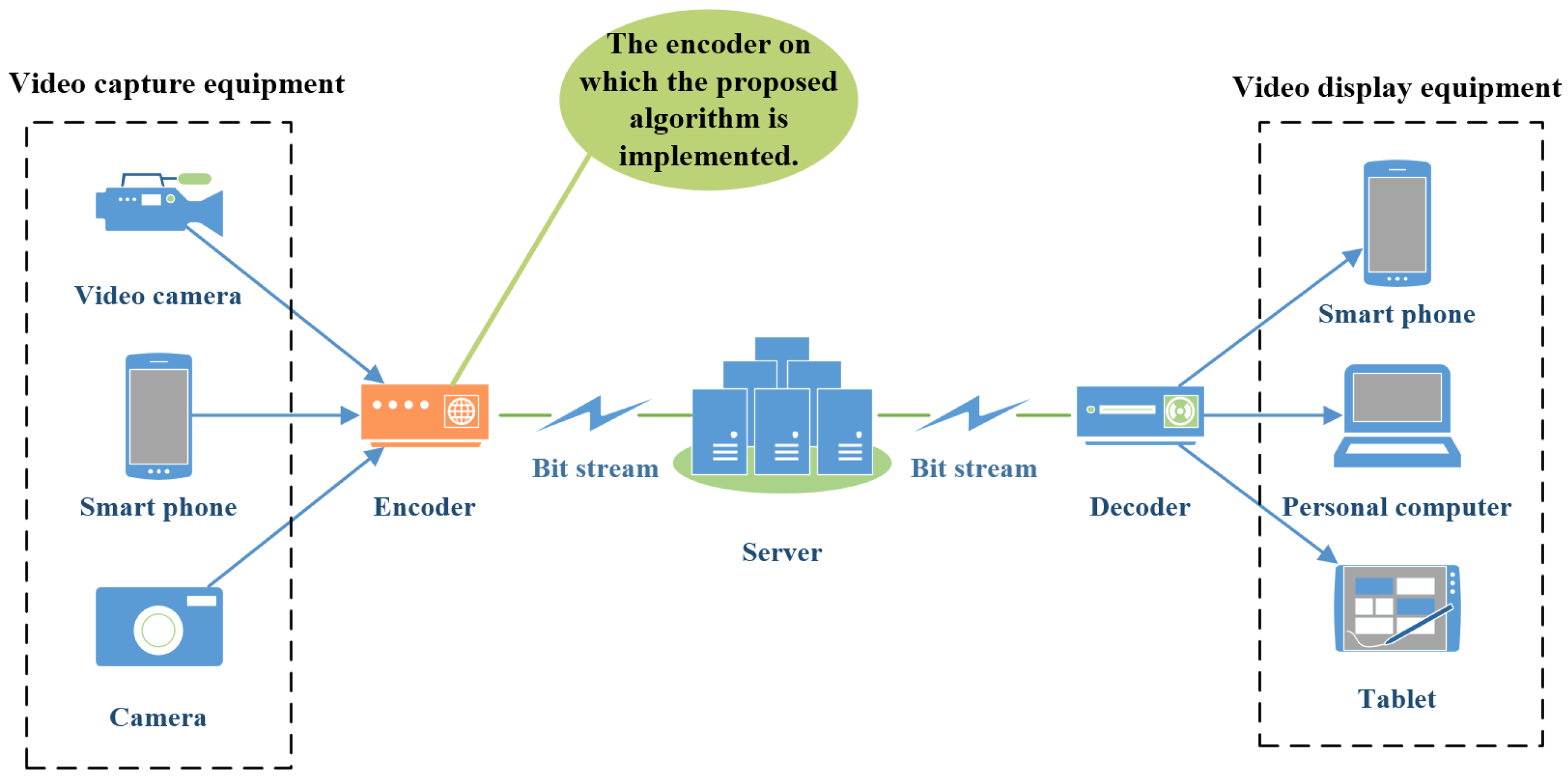
6.5. Application of the Proposed Research

The proposed algorithm has a broad application and plays a very important role in the video dissemination scene of the modern Internet. Figure 15 shows the main process of video from capture to display in Internet, which includes collection, transmission, storage and playback. As we can see from Figure 15, raw videos are collected by various equipment firstly. Then every videos are encoded by the encoder in which the proposed algorithm can be implemented. Thus, to make people have a good viewing experience, the encoder must be fast and of high quality.
To further analyze the application effects of the proposed research, we compare the visual quality of videos encoded by the proposed ABTFA with that of the original HM16.7. Specifically, we encode the 150-th frame of video sequence RaceHorses (416 × 240) under QPs 22, 27, 32, 37, using the ABTFA and the original HM16.7, respectively. Figure 16 shows the visual quality of the frame. Figure 16a–d show the 150-th frame of video sequence RaceHorses (416 × 240) which is encoded by the original HM16.7 under QPs 22, 27, 32, 37, respectively. Figure 16e–h show the 150-th frame of video sequence RaceHorses (416 × 240) which is encoded by the proposed ABTFA with BD-rate loss constraint 0.9% under QPs 22, 27, 32, 37, respectively. We zoom in the pixel block with red boundary in the middle of each sub-picture to observe the details. The details can be observed from the block with red boundary locating at the bottom-right corner in each sub-picture of Figure 16. Observing Figure 16a–d, we can conclude that, for the original HM16.7, the visual quality decreases with the increment of QP. Moreover, we can draw the same conclusion for the proposed ABTFA by observing Figure 16e–h. Besides, there is no visible difference between Figure 16a,e, Figure 16b,f, Figure 16c,g, Figure 16d,h. This observation indicates that there is no obvious application difference between the original HM16.7 and the proposed research. Generally speaking, our algorithm works as well as the original HM16.7, while our algorithm takes much less time.

7. Conclusions

This paper proposes a bagged tree based fast CU size decision algorithm named BTFA with an adaptive threshold calculation method for HEVC intra-coding. Furthermore, a more advanced fast approach called ABTFA is also proposed by employing neural network to optimize the thresholds calculation process. In this work, we design several novel features and perform comprehensive analysis of all the feature candidates. We also design a three-output bagged tree model to deal with the problem of CU partitioning. Besides, an adaptive thresholds calculation method is proposed to further improve the encoding efficiency. Furthermore, an upgraded approach is proposed, in which neural network is used to calculate an optimal result according to a certain constraint of BD-rate loss or time saving. The extensive experimental results demonstrate the effectiveness of our method. Compared with original HM16.7, the proposed BTFA algorithm reduces 41.90% encoding time with only 0.92% BD-rate loss. To our best result, ABTFA achieves an average 47.87% of time saving while the rate-distortion maintains a negligible 0.96%. According to the comparison with some state-of-the-art, the proposed algorithms show great competitive performance. We believe that there is great potential of the proposed ABTFA algorithm to be widely used in industrial applications.
In this paper, our method only focuses on intra-coding rather that inter-coding of HEVC. Actually, inter-coding is more widely used than intra-coding in the actual scene. We will develop the proposed algorithm for inter-coding to achieve improvements in the future.

Author Contributions

Conceptualization, Y.L., L.L. and H.P.; Formal analysis, Y.L. and Y.F.; Software, Y.L. and Y.F.; Supervision, H.P. and Y.Y.; Writing—Original draft preparation, Y.L. and H.P.; Writing—Review and editing, L.L. and Y.Y. All authors have read and agreed to the published version of the manuscript.

Funding

This work is supported by the National Natural Science Foundation of China grant numbers 61932005, 61972051 and 61771071.

Conflicts of Interest

The authors declare no conflict of interest.

Abbreviations

The following abbreviations are used in this manuscript:
HEVCHigh Efficiency Video Coding
BTFABagged Tree based Fast Approach
ABTFAAdvanced Bagged Tree based Fast Approach
CTUCoding Tree Unit
CUCoding Unit
PUPrediction Unit
JCT-VCJoint Collaborative Team on Video Coding
AVCAdvanced Video Coding
RDORate-Distortion Optimization
SVMSupport Vector Machine
SHVCScalable High efficiency Video Coding
RDRate Distortion
BD-rateBit-Distortion rate
BDBRBjontegaard Delta Bit Rate
QPQuantization Parameter
CBFCoded Block Flag
M C R L negative misclassification rate
M C R H positive misclassification rate
G T Ground Truth
PProbability
TThreshold
T L Low Threshold
T H High Threshold
G1Group One
G2Group Two
G3Group Three
G4Group Four
G5Group Five
G6Group Six
DDETthe algorithm proposed by [32]
FADTthe algorithm proposed by [33]
FARFthe algorithm proposed by [34]
DA-SVMthe algorithm poposed by [17]

References

  1. Sullivan, G.J.; Ohm, J.; Han, W.; Wiegand, T. Overview of the High Efficiency Video Coding (HEVC) Standard. IEEE Trans. Circuits Syst. Video Technol. 2012, 22, 1649–1668. [Google Scholar] [CrossRef]
  2. Sullivan, G.J.; Topiwala, P.N.; Luthra, A. The H. 264/AVC advanced video coding standard: Overview and introduction to the fidelity range extensions. In Applications of Digital Image Processing XXVII; International Society for Optics and Photonics: Denver, CO, USA, 2–6 August 2004; pp. 454–474. [Google Scholar]
  3. Sze, V.; Budagavi, M.; Sullivan, G.J. High efficiency video coding (HEVC). In Integrated Circuit and Systems, Algorithms and Architectures; Springer: New York, NY, USA, 2014; pp. 49–90. [Google Scholar]
  4. Sullivan, G.J.; Wiegand, T. Rate-distortion optimization for video compression. IEEE Signal Process. Mag. 1998, 15, 74–90. [Google Scholar] [CrossRef] [Green Version]
  5. Huang, Y.; Wang, D.; Sun, Y.; Hang, B. A fast intra-coding algorithm for HEVC by jointly utilizing naive Bayesian and SVM. Multimed. Tools Appl. 2020, 79, 1–15. [Google Scholar]
  6. Linwei, Z.; Yun, Z.; Kwong, S.; Xu, W.; Tiesong, T. Fuzzy SVM-Based Coding Unit Decision in HEVC. IEEE Trans. Broadcast. 2018, 64, 681–694. [Google Scholar]
  7. Kuo, Y.T.; Chen, P.Y.; Lin, H.C. A Spatiotemporal Content-Based CU Size Decision Algorithm for HEVC. IEEE Trans. Broadcast. 2020, 66, 100–112. [Google Scholar] [CrossRef]
  8. Heidari, B.; Ramezanpour, M. Reduction of intra-coding time for HEVC based on temporary direction map. J. Real-Time Image Process. 2020, 17, 567–579. [Google Scholar] [CrossRef]
  9. Liu, X.; Li, Y.; Liu, D.; Wang, P.; Yang, L.T. An Adaptive CU Size Decision Algorithm for HEVC Intra-Prediction Based on Complexity Classification Using Machine Learning. IEEE Trans. Circuits Syst. Video Technol. 2019, 29, 144–155. [Google Scholar]
  10. Tahir, M.; Taj, I.A.; Assuncao, P.A.; Asif, M. Fast video encoding based on random forests. J. -Real-Time Image Process. 2019, 16, 1–21. [Google Scholar] [CrossRef]
  11. Zhang, J.; Kwong, S.; Wang, X. Two-Stage Fast Inter-CU Decision for HEVC Based on Bayesian Method and Conditional Random Fields. IEEE Trans. Circuits Syst. Video Technol. 2018, 28, 3223–3235. [Google Scholar] [CrossRef]
  12. Chen, Z.; Shi, J.; Li, W. Learned fast HEVC intra-coding. IEEE Trans. Image Process. 2020, 29, 5431–5446. [Google Scholar] [CrossRef] [PubMed] [Green Version]
  13. Kim, K.; Ro, W.W. Fast CU Depth Decision for HEVC using Neural Networks. IEEE Trans. Circuits Syst. Video Technol. 2018, 29, 1462–1473. [Google Scholar] [CrossRef]
  14. Fu, C.H.; Chen, H.; Chan, Y.L.; Tsang, S.H.; Zhu, X. Early termination for fast intra-mode decision in depth map coding using DIS-inheritance. Signal Process. Image Commun. 2020, 80, 115644. [Google Scholar] [CrossRef]
  15. Li, Y.; Zhu, N.; Yang, G.; Zhu, Y.; Ding, X. Self-learning residual model for fast intra-CU size decision in 3D-HEVC. Signal Process. Image Commun. 2020, 80, 115660. [Google Scholar] [CrossRef]
  16. Zhu, L.; Yun, Z.; Pan, Z.; Ran, W.; Kwong, S.; Peng, Z. Binary and Multi-Class Learning Based Low Complexity Optimization for HEVC Encoding. IEEE Trans. Broadcast. 2017, 63, 547–561. [Google Scholar] [CrossRef]
  17. Zhang, Y.; Pan, Z.; Li, N.; Wang, X.; Jiang, G.; Kwong, S. Effective Data Driven Coding Unit Size Decision Approaches for HEVC INTRA Coding. IEEE Trans. Circuits Syst. Video Technol. 2017, 28, 3208–3222. [Google Scholar] [CrossRef]
  18. Moslemnejad, S.; Hamidzadeh, J. A hybrid method for increasing the speed of SVM training using belief function theory and boundary region. Int. J. Mach. Learn. Cybern. 2019, 10, 3557–3574. [Google Scholar] [CrossRef]
  19. Shi, J.; Gao, C.; Chen, Z. Asymmetric-Kernel CNN Based Fast CTU Partition for HEVC Intra-Coding. In Proceedings of the 2019 IEEE International Symposium on Circuits and Systems (ISCAS), Sapporo, Japan, 26–29 May 2019; pp. 1–5. [Google Scholar]
  20. Duarte, D.; Ståhl, N. Machine learning: A concise overview. In Data Science in Practice; Springer: Cham, Switzerland, 2019; pp. 27–58. [Google Scholar]
  21. Wang, D.; Sun, Y.; Zhu, C.; Li, W.; Dufaux, F. Fast depth and inter-mode prediction for quality scalable high efficiency video coding. IEEE Trans. Multimed. 2019, 22, 833–845. [Google Scholar] [CrossRef]
  22. Wang, D.; Zhu, C.; Sun, Y.; Dufaux, F.; Huang, Y. Efficient multi-strategy intra-prediction for quality scalable high efficiency video coding. IEEE Trans. Image Process. 2019, 28, 2063–2074. [Google Scholar] [CrossRef] [PubMed] [Green Version]
  23. Kuang, W.; Chan, Y.L.; Tsang, S.H.; Siu, W.C. Online-learning-based Bayesian decision rule for fast intra-mode and CU partitioning algorithm in HEVC screen content coding. IEEE Trans. Image Process. 2019, 29, 170–185. [Google Scholar] [CrossRef]
  24. Kuang, W.; Chan, Y.L.; Tsang, S.H.; Siu, W.C. Machine Learning-Based Fast Intra-Mode Decision for HEVC Screen Content Coding via Decision Trees. IEEE Trans. Circuits Syst. Video Technol. 2019, 30, 1481–1496. [Google Scholar] [CrossRef]
  25. Fu, B.; Zhang, Q.; Hu, J. Fast prediction mode selection and CU partition for HEVC intra coding. IET Image Process. 2020, 14, 1892–1900. [Google Scholar]
  26. Utgoff, P.E.; Berkman, N.C.; Clouse, J.A. Decision Tree Induction Based on Efficient Tree Restructuring. Mach. Learn. 1997, 29, 5–44. [Google Scholar] [CrossRef] [Green Version]
  27. Shen, X.; Yu, L. CU splitting early termination based on weighted SVM. EURASIP J. Image Video Process. 2013, 2013, 4. [Google Scholar]
  28. Grellert, M.; Bampi, S.; Correa, G.; Zatt, B.; da Silva Cruz, L.A. Learning-based complexity reduction and scaling for HEVC encoders. In Proceedings of the 2018 IEEE International Conference on Acoustics, Speech and Signal Processing (ICASSP), Seoul, South Korea, 22–27 April 2018; pp. 1208–1212. [Google Scholar]
  29. Bay, H.; Ess, A.; Tuytelaars, T.; Van Gool, L. Speeded-Up Robust Features (SURF). Comput. Vis. Image Underst. 2008, 110, 346–359. [Google Scholar]
  30. Caruana, R.; Elhawary, M.; Munson, A.; Riedewald, M.; Sorokina, D.; Fink, D.; Hochachka, W.M.; Kelling, S. Mining citizen science data to predict orevalence of wild bird species. In Proceedings of the 12th ACM SIGKDD International Conference on Knowledge Discovery and Data Mining, Philadelphia, PA, USA, 1 August 2006. [Google Scholar]
  31. Bossen, F. Common test conditions and software reference configurations. In Proceedings of the Joint Collaborative Team on Video Coding of ITU-T SG16 WP3 and ISO/IEC JTC1/SC29/WG11, Geneva, Switzerland, 21–28 July 2010. [Google Scholar]
  32. Zhang, Y.; Kwong, S.; Zhang, G.; Pan, Z.; Yuan, H.; Jiang, G. Low Complexity HEVC INTRA Coding for High-Quality Mobile Video Communication. IEEE Trans. Ind. Inform. 2015, 11, 1492–1504. [Google Scholar] [CrossRef]
  33. Zhu, S.; Zhang, C. A fast algorithm of intra-prediction modes pruning for HEVC based on decision trees and a new three-step search. Multimed. Tools Appl. 2016, 76, 21707–21728. [Google Scholar]
  34. Du, B.; Siu, W.C.; Yang, X. Fast CU partition strategy for HEVC intra-frame coding using learning approach via random forests. In Proceedings of the Asia-Pacific Signal and Information Processing Association Summit and Conference, Jeju, Korea, 13–16 December 2016. [Google Scholar]
Figure 1. A splitting example of a coding unit (CU) in intra-coding. Left part shows the final splitting result of a CU. Right part is the corresponding structure of quad-tree, in which black solid lines are CU splitting branches and dot red lines are splitting branches for prediction units (PUs).
Electronics 09 01523 g001
Figure 2. Structures of decision tree and bagged tree. (a) a simple structure of a decision tree, in which Feature_n represents the nth feature and Threshold_n is the corresponding threshold to make a decision. Each leaf node represents a class label and each father node represents a judging process. (b) a structure of bagged tree model. n is the number of decision trees used to make up a bagged tree, and D T _ n presents the nth decision model among them. O u t p u t _ n is the output of the nth decision tree model, and it is used to calculate the final output of bagged tree.
Electronics 09 01523 g002
Figure 3. Framework of the proposed frame-wise beforehand prediction. Frame n represents the n-th frame in a video sequence to be encoded. t n represents the time t n , at which the process happens. Blocks in the same color happen at the same time.
Electronics 09 01523 g003
Figure 4. Flowchart of the proposed BTFA. Value 0 of splitFlag represents a nonsplit decision of a CU, while the values 1 and 2 are split and RDO decision, respectively.
Electronics 09 01523 g004
Figure 5. Sobel filters among different directions. (a) an example of original pixels for a 3 × 3 block within a CU. (b) a horizontal edge filter. (c) a vertical edge filter. (d,e) the extended filters for 45 ° and 135 ° , respectively.
Electronics 09 01523 g005
Figure 6. Three filters used in interest point detection for horizontal, vertical and diagonal direction. D x x is the horizontal filter, D y y is the vertical filter and D x y is used to detect diagonal interest points. Each filter is performed on every pixel in a CU with overlap.
Electronics 09 01523 g006
Figure 7. Haar filters for different directions. (a) An example of an original 2 × 2 pixel block, on which each Haar filter is performed. (b) The horizontal Haar filter, (c) the vertical Haar filter and (d) the diagonal Haar filter; (bd) will be applied on a, b, c and d to generate the corresponding Haar responses of different directions.
Electronics 09 01523 g007
Figure 8. Importance values of 32 feature candidates for 20 classifier models. Axis x is the categories of a bagged tree model, e.g., 22-A is the bagged tree model trained for sequences in QP 22 and resolution class A. Axis y represents features whose serial number is the corresponding index in Table 1, e.g., feature of No. 15 is m_costHadamard.
Electronics 09 01523 g008
Figure 9. Classification edge of binary output and three-output classifiers. Class 0 represents non-split CUs, while class 1 represents splitting and class 2 is the CU category in which rate-distortion optimization (RDO) is performed. Red line is the classification edge between different categories.
Electronics 09 01523 g009
Figure 10. Flowchart of adaptive thresholds calculation method. P is the splitting probabilities of samples, and it is the output of classifier. T is possible thresholds used to generate a predicted CU label. P L represents the predicted labels of samples, and it is transferred from P with T. G T is the ground truth of samples. Part I is the mapping process from the probabilities to the predicted labels. Part II is the confusion matrix calculation process according to P L and G T . Part III illustrates the thresholds determination according to misclassification rates with corresponding thresholds. Blocks in the same color are the results generated under the same value of T.
Electronics 09 01523 g010
Figure 11. Surface of Bit-Distortion (BD)-rate loss and time saving in the training set with respect to T L 1 , T H 1 and T L 2 , T H 2 . (a) the surface of BD-rate loss with respect to T H 1 and T L 1 . (b) the surface of time saving with respect to T H 1 and T L 1 . (c) the surface of BD-rate loss with respect to T H 2 and T L 2 . (d) the surface of time saving with respect to T H 2 and T L 2 .
Electronics 09 01523 g011
Figure 12. Structure of neural network used to fit the mathematical relation among BD-rate loss, time saving and thresholds. Number under blocks represents the number of neurons in corresponding layer.
Electronics 09 01523 g012
Figure 13. Partition result of the 200th frame in sequence BasketballPass, which is encoded by original HM16.7 under QP 22. Solid black line represents the partition result of CUs.
Electronics 09 01523 g013
Figure 14. Partition result of the 200th frame in sequence BasketballPass encoded under QP 22 by encoder HM16.7, in which the proposed ABTFA with BD-rate loss constraint 0.9% is applied. Black line represents the same partition results as those of original HM16.7. Green line represents boundaries of CUs, which are split by original HM16.7 but are not split by ABTFA. Boundaries of CUs, that are decided non-split by original HM16.7 but are split by ABTFA, are shown with red line.
Electronics 09 01523 g014
Figure 15. The application of the proposed research. Part in orange is where our algorithm works.
Electronics 09 01523 g015
Figure 16. Visual quality comparison of videos encoded with different Quantization Parameter (QPs) by the original HM16.7 and the encoder in which the proposed ABTFA with BD-rate loss constraint 0.9% is applied. (ad) the 150-th frame of video sequence RaceHorses (416 × 240) which is encoded by the original HM16.7 under QPs 22, 27, 32, 37, respectively. (eh) the 150-th frame of video sequence RaceHorses (416 × 240) which is encoded by the proposed ABTFA with BD-rate loss constraint 0.9% under QPs 22, 27, 32, 37, respectively. We zoom in the block with red boundary in the middle of each sub-picture to observe the details. The details can be observed from the block with red boundary locating at the bottom-right corner in each sub-picture.
Electronics 09 01523 g016
Table 1. Feature candidates taken into account
IndexFeature CandidatesFeature Description
1 m _ v a r M e a n S u b variance of four sub CUs’ mean
2 m _ v a r V a r S u b variance of four sub CUs’ variance
3 m _ a v e C B F average value of current CU’s Coded Block Flag
4 m _ n b C t u A b o R d RD cost of current CU’s above CTU
5 m _ n b C t u L e f R d RD cost of current CU’s left CTU
6 m _ n b C t u A b l R d RD cost of current CU’s above left CTU
7 m _ n b C t u A b r R d RD cost of current CU’s above right CTU
8 m _ n b C t u A b o D e p t h depth of current CU’s above CTU
9 m _ n b C t u L e f D e p t h depth of current CU’s left CTU
10 m _ n b C t u A b l D e p t h depth of current CU’s above left CTU
11 m _ n b C t u A b r D e p t h depth of current CU’s above right CTU
12 t o t a l C o s t total cost of current CU encoded with planar
13 t o t a l D i s t o r t i o n total distortion of current CU encoded with planar
14 t o t a l B i n s total bins of current CU encoded with planar
15 m _ c o s t H a d a m a r d hadamard cost of planar mode
16 m _ s a d H a d a m a r d distortion of residual after hadamard transfer
17 m _ b i t s H a d a m a r d hadamard bits of planar mode
18 m _ e d g e S o b e l edge detection result using Sobel
19 m _ n m s e mean square error of neighbor pixels
20 m _ d c o m mean of gradients of four directions
21 m _ n u m I n t e r e s t P o i n t number of interesting points of current CU
22 m _ h a a r S u m x sum of horizontal value after Haar wavelet transfer
23 m _ h a a r S u m y sum of vertical value after Haar wavelet transfer
24 m _ h a a r S u m x y sum of diagonal value after Haar wavelet transfer
25 m _ h a a r S u m A b s x sum of horizontal absolute value after Haar
26 m _ h a a r S u m A b s y sum of vertical absolute value after Haar
27 m _ h a a r S u m A b s x y sum of diagonal absolute value after Haar
28 m _ m e a n M a i n mean of current CU
29 m _ v a r M a i n variance of current CU
30 d e p t h C l a s s 1 if current depth is 0
31 d e p t h C l a s s 2 if current depth is 1
32 d e p t h C l a s s 3 if current depth is 2
Table 2. Prediction accuracy of CUs in different depth.
ClassSequenceQPPrediction Accuracy
Depth0Depth1Depth2
ATraffic
(2560 × 1600)
2286.80%82.50%79.71%
2791.76%84.19%77.35%
3287.36%82.63%70.05%
3779.17%79.19%75.00%
BParkScene
(1920 × 1080)
2286.34%81.17%77.65%
2788.66%85.14%77.27%
3288.50%83.98%75.33%
3785.77%79.99%74.54%
CBasketballDrill
(832 × 480)
2299.87%91.39%70.84%
2799.49%77.89%70.74%
3298.33%74.36%77.40%
3792.27%76.83%84.23%
DBQSquare
(416 × 240)
2299.91%91.29%85.90%
2798.86%93.10%90.86%
3298.24%94.42%91.09%
3796.65%94.68%91.35%
EFourPeople
(1280 × 720)
2293.17%85.04%80.85%
2794.20%89.54%79.88%
3294.88%88.55%79.46%
3792.86%85.06%78.47%
Average92.65%85.05%79.40%
Table 3. Confusion matrix of the proposed bagged tree model
Predicted Label
01
True
Label
0true
negative ( T N )
false
positive ( F P )
1false
negative ( F N )
true
positive ( T P )
Table 4. BD-rate loss and time saving results of bagged trees based fast approach (BTFA) under different threshold groups.
ClassSequenceBTFA-G1BTFA-G2BTFA-G3BTFA-G4BTFA-G5
BD-Rate
(%)
TS
(%)
BD-Rate
(%)
TS
(%)
BD-Rrate
(%)
TS
(%)
BD-Rate
(%)
TS
(%)
BD-Rate
(%)
TS
(%)
ATraffic0.5731.820.7238.260.9135.431.0340.090.9738.54
PeopleOnStreet0.5030.340.5834.901.1135.481.1638.061.1538.67
Average0.5331.080.6536.581.0135.461.0939.071.0638.61
BKimono1.9855.952.0057.313.3158.513.3259.233.3358.95
ParkScene0.3531.010.4837.610.5735.210.6739.690.6337.84
Cactus0.5734.800.8442.330.8939.501.1144.950.9942.50
BasketballDrive1.5841.251.7046.442.3545.172.4649.092.4047.85
BQTerrace0.5239.090.6845.461.0644.311.0946.881.1849.22
Average1.0040.421.1445.831.6444.541.7347.971.7147.27
CBasketballDrill0.2325.410.5130.910.4628.880.6733.240.5531.30
BQMall0.3132.120.9741.520.4535.010.9741.520.6338.96
PartyScene0.4930.471.5637.560.5134.341.3637.680.7938.95
RaceHorses0.2836.740.5845.850.3840.390.6047.490.5043.71
Average0.3331.180.9038.960.4534.660.9039.980.6238.23
DBasketballPass0.1729.360.4036.590.4732.270.6736.340.5735.14
BQSquare0.3535.461.2640.000.4136.791.1838.640.5739.25
BlowingBubbles0.0122.700.1625.760.0525.070.1425.950.1126.93
RaceHorses0.2527.200.8233.290.2930.110.7333.760.4832.86
Average0.2028.680.6633.910.3131.060.6833.670.4333.55
EFourPeople0.3437.180.7444.960.8941.871.1447.651.0845.87
Johnny0.9155.171.3261.622.1558.492.3863.132.4162.23
KristenAndSara0.8649.101.2156.381.8952.562.0958.572.1955.90
Average0.7047.151.0954.321.6550.971.8756.451.8954.67
Overall Average0.5735.840.9242.041.0139.411.2643.441.1442.48
G1 represents group 1 for values of MCRL1, MCRH1, MCRL2 and MCRH2, and it is set as [0.02, 0.03, 0.02, 0.03]. G2 is [0.07, 0.03, 0.07, 0.03]. G3 is [0.02, 0.08, 0.02, 0.08]. G4 is [0.07, 0.08, 0.02, 0.08]. G5 is [0.02, 0.08, 0.07, 0.08].
Table 5. BD-rate loss and time saving of advanced bagged trees based fast approach (ABTFA) under different target BD-rate loss constraint and target time saving constraint.
ClassSequenceABTFA
B L tar = 0.6%
ABTFA
T S tar = 45%
B
T S tar  = 50%
BD-Rate
(%)
TS
(%)
BD-Rate
(%)
TS
(%)
BD-Rate
(%)
TS
(%)
ATraffic0.9432.871.7444.643.4962.12
PeopleOnStreet0.9132.041.7543.683.0154.99
Average0.9232.451.7444.163.2558.55
BKimono1.2356.051.8766.803.3678.40
ParkScene0.6332.951.1244.182.4061.01
Cactus0.8934.421.4345.072.7460.30
BasketballDrive1.6743.172.5855.224.3867.74
BQTerrace0.7939.321.0946.531.6054.03
Average1.0441.181.6251.562.8964.30
CBasketballDrill0.2524.531.1439.103.7158.12
BQMall0.3832.251.1244.212.5557.08
PartyScene0.1031.570.3636.990.8543.47
RaceHorses0.4139.260.9651.761.8562.84
Average0.2831.900.8943.022.2455.38
DBasketballPass0.2030.910.8241.441.7649.75
BQSquare0.0830.030.2135.360.4239.52
BlowingBubbles0.0625.820.2530.360.5134.56
RaceHorses0.1630.290.6037.911.3145.56
Average0.1329.260.4736.271.0042.35
EFourPeople1.1536.201.8547.203.0659.58
Johnny1.2654.972.1563.233.6970.82
KristenAndSara1.1546.711.7857.043.3568.15
Average1.1945.961.9355.823.3766.19
Overall Average0.6836.301.2746.152.4557.11
Table 6. BD-rate loss and time saving comparison between the proposed BTFA, ABTFA and state-of-the-art.
ClassSequenceDDETFADTFARFDA-SVMBTFA-G6ABTFA
(B L tar = 0.9)
BD-Rate
(%)
TS
(%)
BD-Rate
(%)
TS
(%)
BD-Rrate
(%)
TS
(%)
BD-Rate
(%)
TS
(%)
BD-Rate
(%)
TS
(%)
BD-Rate
(%)
TS
(%)
ATraffic0.7239.751.2738.960.9044.800.9845.690.8038.061.0148.66
PeopleOnStreet0.5236.231.0338.060.6040.601.2044.810.8036.420.5942.54
Average0.6237.991.1538.510.7542.701.0945.250.8037.240.8045.60
BKimono1.0055.262.2239.661.8076.103.7280.532.5057.921.9972.06
ParkScene0.7337.791.0037.900.6047.000.6740.010.5037.890.8248.43
Cactus1.3242.050.7334.830.7045.801.0245.500.8042.591.0249.00
BasketballDrive0.6748.071.6940.571.8063.401.8761.091.9045.992.2058.21
BQTerrace1.0346.961.0038.500.3047.801.0551.030.8045.630.6244.97
Average0.9546.031.3338.291.0456.021.6755.631.3046.001.3354.54
CBasketballDrill0.3631.071.3837.990.6038.100.9939.740.5032.281.5044.12
BQMall1.0536.100.4836.930.2035.301.0738.380.7040.181.1046.49
PartyScene0.9130.770.3236.010.0031.200.2428.821.2037.570.3235.92
RaceHorses1.8628.500.7138.670.4037.901.1840.110.5043.940.9454.51
Average1.0531.610.7237.400.3035.630.8736.760.7338.490.9645.26
DBasketballPass0.9141.211.5434.291.1048.201.3445.990.4036.290.8643.76
BQSquare1.3223.380.6540.310.1039.900.5036.290.8039.250.1735.60
BlowingBubbles0.4221.450.6329.680.2038.200.4827.950.1026.270.1728.50
RaceHorses 1.1430.690.1033.10 0.6033.160.5736.93
Average0.8828.680.9933.740.3839.850.7736.740.4833.740.4436.20
EFourPeople1.0943.730.3940.750.6040.001.7051.760.8044.010.7847.07
Johnny1.1755.942.6245.751.9057.103.0167.991.6061.651.4064.21
KristenAndSara1.1554.781.9242.151.3052.302.3963.561.5056.411.2360.73
Average1.1451.481.6442.881.2749.802.3761.101.3054.021.1457.34
Overall Average0.9539.591.1537.871.3052.301.3847.600.9241.900.9647.87
Table 7. BD-rate loss and time saving comparison between the proposed algorithm and the most recent works.
SequenceHuang [5]Liu [9]Fu [25]BTFA-G1ABTFA( B L tar = 0.9)
BD-Rate (%)TS (%)BD-Rate (%)TS (%)BD-Rate (%)TS (%)BD-Rate (%)TS (%)BD-Rate (%)TS (%)
BasketballDrill1.0248.231.0643.251.4942.200.2325.411.5044.12
BasketballDrive1.4365.371.3850.731.3259.801.5841.252.2058.21
Johnny1.8966.211.9363.151.4562.900.9155.171.4064.21
KristenAndSara1.6567.411.6859.251.1759.200.8649.101.2360.73
ParkScene0.7449.860.7945.210.7248.300.3531.010.8248.43
Average1.3459.411.3652.311.2354.480.7840.381.4355.14

