Guided Networks for Few-Shot Image Segmentation and Fully Connected CRFs

Abstract

The goal of the few-shot learning method is to learn quickly from a low-data regime. Structured output tasks like segmentation are challenging for few-shot learning, due to their being high-dimensional and statistically dependent. For this problem, we propose improved guided networks and combine them with a fully connected conditional random field (CRF). The guided network extracts task representations from annotated support images through feature fusion to do fast, accurate inference on new unannotated query images. By bringing together few-shot learning methods and fully connected CRFs, our method can do accurate object segmentation by overcoming poor localization properties of deep convolutional neural networks and can quickly updating tasks, without further optimization, when faced with new data. Our guided network is at the forefront of accuracy for the terms of annotation volume and time.

1. Introduction

In the context of deep learning, each class requires at least thousands of training samples to saturate the performance of convolutional neural networks on known categories. In addition, the generalization ability of neural networks is weak. When the novel class comes, it is difficult for the model to learn to identify novel concepts through a small number of labeled samples. However, humans have the ability to quickly learn from small (single) samples. People can even accurately identify things in a picture based on just one picture. Inspired by the rapid learning ability of human beings, the researchers hope that the machine learning model can learn quickly after learning a large amount of data of a certain category, and only a small sample is needed for the new category. These prompted the emergence of few-shot learning methods [1,2,3]. The current few-shot learning methods mainly rely on meta-learning to adapt to new tasks. However, these methods focus on classification rather than structured output tasks.

Image segmentation is the core task of visual recognition, and its end-to-end system has achieved advanced performance. Although deep convolution neural network (DCNN) has made great progress in the field of image segmentation, there is evidence that the response of the last layer of DCNN is not enough to accurately locate the target boundary [4]. Convolution neural network models perform very poorly in their ability to capture fine edge details and are unable to adapt to long-range dependencies. In order to solve the problem of small amount of training data and precise segmentation at the same time, we propose combining the few-shot learning method with fully connected pairwise conditional random fields (CRFs) proposed by Krähenbühl and Koltun [5], for its efficient computation and localization performance.

Specifically, we solve such a few-shot segmentation problem: just a little sparse pixelwise annotated support images for indicating the task are given, and then segment unannotated images correspondingly. In this work, our framework is at the pixel-level. That is to say, the input and output are all the pixel-level. Thus, they are from inside and across images propagating pixel annotations to unannotated pixel for inference. In addition, we can infer the latent task representation defined by sparse pixelwise annotations through optimizing the guided network. Moreover, according to the latent task representation, the new query image without pixel annotations is segmented accordingly. Our guided network even requires only two annotated pixels (one positive pixel and one negative pixel) per concept, to segment new concepts, and incorporates further annotations to renew and ameliorate inference. Our method can spread across the spectrum from an annotated pixel to intensive entire masks, unlike some existing methods that may fail to segment specific tasks in very sparse regimes.

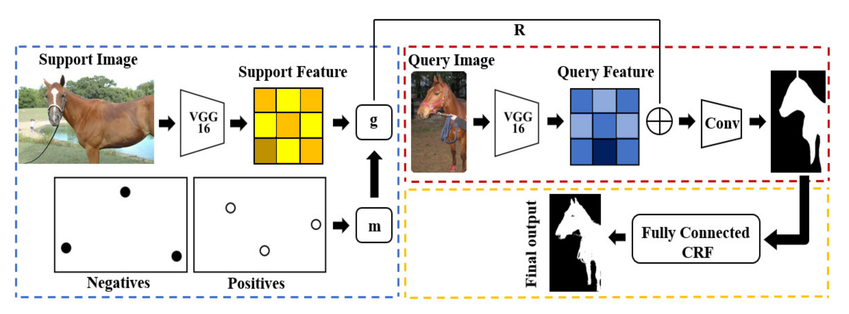
In this paper, we propose a new class of guided networks which combines fully connected CRFs (see Figure 1). Our model is composed of three fairly well-established branches, guided branch, segmentation branch, and fully connected CRFs. Given an annotated support set, the guide (g) extracts a potential task representation (R) and uses it to direct the segmentations of query images. We introduce a new mechanism for merging images and annotations on encode the support, which greatly improves learning time and inference accuracy. For the segmentation branch, we designed a small convolutional network, which can be understood as a learning distance measure from support to query; under the guidance of task representation, R, the segmentation branch extracts the foreground object of the image and generates rough segmentation results. Once trained, our model does not need to make further efforts to optimize to deal with new few-shot tasks. Finally, we use fully connected CRFs to optimize the details of the output and pinpoint it.

The main contributions of this paper can be summarized as the following three aspects: (1) We implemented an image segmentation algorithm which combines the few-shot learning method and the fully connected conditional random field (CRF), and get relatively good segmentation results; (2) we introduce a new mechanism for merging images and annotations, to improve learning time and inference accuracy and propagate pixels across different images; and (3) we combined the fully connected CRF behind the guided network, to improve the ability of the network to capture detailed features and achieve accurate segmentation of objects.

2. Related Work

Our framework realizes the accurate segmentation of images with a little training samples. At present, deep learning technology has made tremendous progress in the field of image segmentation [6,7,8,9]. However, due to the bottleneck of deep learning technology, which needs a large amount of label data, it has led to the exploration of the few-shot learning method. We concentrate on one-shot, semi-supervised, and interactive methods; at the same time, we review the relationship between few-shot learning methods and structured output.

2.1. Few-Shot Learning

The few-shot learning method is a good generalization for the problem of limited labeled datasets, which generally contain only a few training samples of the target class [10]. Although the interest in few-shot learning methods is increasing, most of the current research focuses on classification [11,12,13] rather than structured output, and little attention is paid to the supervision of sparse and imbalanced. Shaban et al. [14] were the first to apply the one-shot learning method to image semantic segmentation, which only requires an image and its corresponding pixel-level annotation per class. Few-shot learning ensures the efficiency of data; at the extreme, one-shot learning requires only a single annotation of a new concept.

To locate our study, we herein review methods such as segmentation associated with visual structured output tasks. During inference, few-shot learning methods do optimize by gradients on a learned recurrent optimizer [15,16]. Notably, the majority scarcely use task and architecture presumptions, but these ways are unconfirmed for the skewed distributions and high dimensionality of segmentation. Motivated by Siamese networks [17] used for metric learning [18,19], few-shot also as embedding learns a metric and seeks the nearest target from the support. Although these mediums are quickly and fairly uncomplicated [20] on small datasets, they are a disgrace with higher shot and way. It is difficult to extend one-shot to few-shot, because of the way of few-shot regresses model parameters based on the support.

2.2. Segmentation

There are many types of segmentation, e.g., semantic segmentation, instance segmentation, panoramic segmentation, and so on. We take the semantic and interactive segmentation as our main challenges (see Figure 2).

The fully convolutional network (FCN) [6] is a pioneering work that applies a convolutional neural network (CNN) structure to the field of image semantic segmentation and achieves outstanding segmentation results. However, its segmentation results are not precise enough to segment the details of the target image. For semantic segmentation, Shaban et al. [14] designed a segmented architecture for one-shot learning method, which only needs a few training images, but requires dense annotations and supervision at training time. For our guided architecture, we only need to randomly point a few positive sample points and negative sample points (foreground points and background points of images) on the training sample image. We mainly draw support from the feedforward guidance for few-shot learning, so as to make our methods faster and better. For interactive segmentation, Xu et al. [21] introduced a state-of-the-art segmentation method. They put the original image together with Euclidean distance maps based on foreground and background annotations into a full convolutional network, to generate a probability map. It is a pity that it cannot propagate pixel annotations across different images. Undeniably, that is a bottleneck on annotation efficiency. What is amazing is that our approach can segment new inputs independently. Thus, even if support images and query images are different, we can also achieve accurate segmentation. This is much better than interactive seg; Xu et al. [21] and we regard the interactive as a special case of few-shot.

2.3. Fully Connected CRFs

Structured prediction tasks such as image segmentation can gain many advantages from conditional random fields and other probability graph models. CRF are often used for pixel-level label prediction. Traditionally, a CRF was used to smooth the noise segmentation images [22,23]. Generally, these models contain energy terms that couple adjacent nodes so that the same labels are assigned to the proximal pixels in space. The basic CRF model is a graph model composed of the unary potential function and the potential function composed of adjacent elements. Obviously, a disadvantage of the basic CRF model in image tasks is that it only considers the adjacent neighborhood elements, without considering the whole, so it will lose some context information. Therefore, a further idea was born: Each pixel is made into an edge for all other pixels, to achieve a dense fully connected model, that is, fully connected CRFs [5]. The fully connected CRF obtains as much adjacent point information as possible by operating all nodes, thereby obtaining more accurate segmentation results [9,24,25].

3. Few-Shot Segmentation

In the few-shot learning method, the training set contains many categories, and there are multiple samples in each category. In the training phase, N classes of data are randomly selected from the training set, and K samples of each class (N × K data in total) are constructed to a meta-task as the model’s support set input. Then, we take a batch of samples from the remaining data of these N classes as the query set of the model. That is to say, the model is required to learn how to distinguish these N classes from N × K data. Such a task is called the N-way, K-shot problem [10,15,26]. For few-shot image segmentation tasks, in this setting, we also need to add a further pixel dimension, as annotations may be spatially dense or sparse. We have to consider the amount of support images and the amount of annotated pixels per support image. We express the amount of pixel annotations for every support image as P and think over the place settings of (K, P)-shot learning for different K and P. We especially pay attention to the sparse annotation, that is, the case where P is very little, because this can reduce the cost of annotation and more practical to collect. More importantly, it only asks the user to point to the segment of interest. Furthermore, we deal with mixed-shot learning, where the quantity of annotation changes as class and task change.

We follow and expand the notation of Chen. et al. [27]. We represent the support and Query set of the task as the following form. Support Set: $Ds={\left\{\left(I_s^i,L_s^i\right)\right\}}_{\mathrm{i}=1}^{N_s}\left(l\right)$ and Query Set: $D_q={\left\{\left(I_q^i,L_q^i\right)\right\}}_{\mathrm{i}=1}^{N_q}\left(l\right)$, where $I^i$ represents the i (th) original image, $L^i$ are the corresponding annotations, the indexes s and q are the support set and query set, N is the number of images in each set, and $\left(l\right)$ is the semantic class of the dataset.

In general, we regard each segmentation task to be binary with $N=2$, or $L=\left(L_{+},L_{-}\right)$, where every task interprets its own positive and negative is the supplement (that is the background in image segmentation). Note that the binary task is a natural one for interactive segmentation problem, in case the tasks consist of a single object to be segmented. Obviously, the binary task can be extended to the higher-way task. Because the inference for every query image is independent in our mechanism, we keep the number of unannotated query images is one.

In order to solve the problem of few-shot image segmentation, our model is divided into three parts:(1) extracting task representation from semi-supervised support images that can express segmentation tasks with high quality; (2) segmenting query images according to the task representation extracted in the previous step; and (3) introducing the fully connected conditional random fields [4], to consider the global location information, and further optimizing the segmentation results. We express the task representation as follows $R=g\left(I_s,L_{+},L_{-}\right)$ and the query segmentation as $y=f\left(I_q,R\right)$. The selection of the task representation, R, and its encoder, $g$, are important for few-shot segmentation to deal with the hierarchical structure of images and their pixelwise annotations. We discuss the issue in Section 4. According to the task representation, we integrate the few-shot methods into the dense pixelwise inference through a fully convolutional network. Compared with other few-shot methods, our evaluation emphasizes the limits of shot and efficiency.

4. Methods

Our model can make predictions independently, while guiding the task and rectifying errors under the guidance of users. Unlike static model parameters, our guidance is dynamically variable. It can be expanded or rectified as directed by an annotator. It is worth noting that the process of self-prediction could be considered as interactive segmentation when the support image and query image are the same. It can be seen as a special case of few-shot segmentation. Specifically, we use a guide, $R=g\left(I_s,L_s\right)$, to extract a latent task representation, R, from the support through the guided branch. Subsequently, the segmentation branch combines task representation, R, and query features to make joint predictions, $y=f\left(I_q,R\right)$. We discuss how to better design the above two function formulas in the following sections.

Our model uses VGG-16 [28] as a feature extractor, pre-training it on ImageNet Large Scale Visual Recognition Challenge (ILSVRC) [29], and converting it into fully convolutional form.

4.1. Guided Branch: Extracting Task Representation from Support

For the sake of the segmentation of query images, the task representation, R, has to fuse pixel annotations with the support image features. Because pixels are semi-supervised and spatially correlated, our support is dependent statistically. In addition, the full supervision is difficult to annotate because of the high-dimensional and class-skewed scenes. For the purpose of simplicity, let us first think over (1, P)-shot support, and then extend it to (K, P)-shot support. We express the guidance process as follows:

$$R=g\left(I_s,L_{+},L_{-}\right)=\mu \left(\lambda \left(I_s\right),m\left(L_{+}\right),m\left(L_{-}\right)\right)$$

(1)

by architecturally inducing structure, where R includes both foreground object features and background features.

Inspired by the method Rakelly et al. proposed [30,31], we first match positive annotated pixels and negative annotated pixels to the same coordinate scale as the support image $I_s$. We record the position of them and set the click position to 1 and others to 0. Afterward, we gain two annotation masks, $\left(L_{+}\right)$ and $\left(L_{-}\right)$,$L\in \left\{0,1\right\}$. Then, we use the pre-trained VGG-16 model as a feature extractor, $\lambda$, to extract visual features from the support alone. Since the VGG-16 model contains 5 pooling operations, the extracted support feature map is reduced by 32 times. To make sure they are the same size, the positive mask and negative mask are both down-sampled by bilinear interpolation kernel $m\left(L_{+}\right),m\left(L_{-}\right)$. Finally, we use the element-wise product, $\mu$, to fuse the support features with the positive mask and negative mask. In this way, we can update the task representation quickly by constantly recomputing the masking, to incorporate new positive and negative annotations. This greatly reduces inference time. Additionally, support and query share a feature extractor to extract visual features, which significantly improves learning efficiency. The overview is shown in Figure 3.

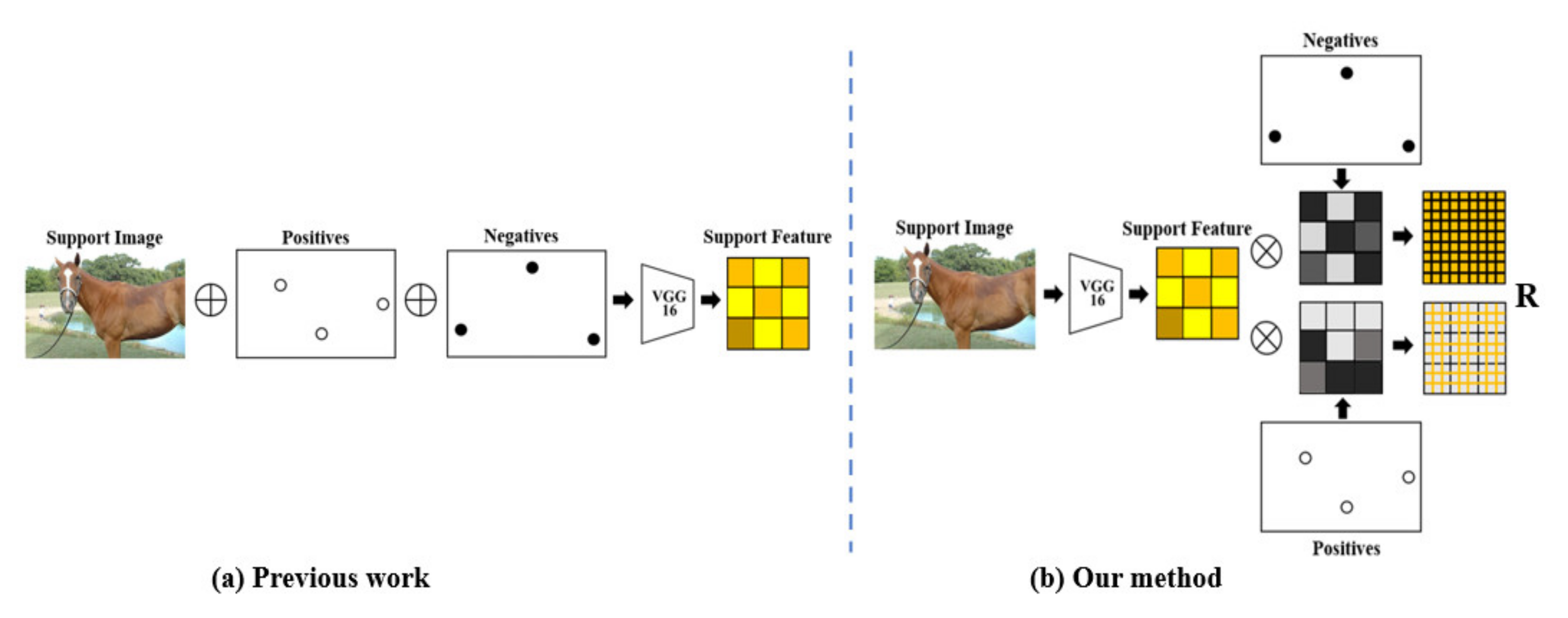
Previous work merely concatenates the image and annotations. Xu et al. [21] proposed a method that enables end-to-end learning to fully control how to fuse. However, due to the fact that the number of channels has changed after concatenating the image and annotations, the original feature extractor VGG-16 cannot handle the new input data. This will break the input structure of the network and prevent the implementation of a unified network. Shaban et al. [14] used the method of directly multiplying the support and dense label annotation to fuse, which ignores all background information. Our method can well preserve the background information of the support. Moreover, the factorization into feature-level information and annotation branches better defines the spatial dependency between annotations and the support. The previous methods have some inherent model problems: inconsistency of the support with query features, and the fusion is so slow.

When there are multiple foreground objects in the image, we hope to segment all the target objects in the image, not just one of them, as shown in Figure 4. In addition, if the support and query images are totally different, the spatial corresponding relationship between the two is unknown, and the support and query images can only be mapped through features. For this, our method is to global pool, to merge the local task representations for all position and abandon the spatial dimensions. In the pooling step, we choose global average pooling to handle it. However, if the support is the same as the query image (e.g., interactive segmentation), feature location is informative, and the global pooling process can be ignored.

4.2. Segmentation Branch: Feature Fusion

In the ordinary fixed segmentation model, the form of inference is just $y=f_{\theta }\left(I_q\right)$ for input image, $I_q$, parameters, $\theta$, and output results, $y$. However, in our method, guided inference is the further function $y=f_{\theta }\left(I_q,R\right)$, where $R$ is the guidance extracted from the support. We use a fusion operation, $C$, to concatenate the guided task representation and the query features. The segmentation process can be defined as follows:

$$y=f_{\theta }\left(C\left(\lambda (I_q\right),R\right))$$

(2)

where $\lambda$ is the same fully convolutional encoder as the support uses. See Figure 5 for a schematic illustration. Specifically, fusion operation, $C$, has this from $C=\lambda \left(I_q\right)\otimes tile\left(r\right)$, where $r$ is the task representation after global pooling obtained by the guided branch. $Tile$ function copies the original matrix horizontally and vertically. $\otimes$ represents the channel numbers stack. We keep repeating the guidance vector, $r$, until it is the same as the spatial dimension of the query features, $\lambda \left(I_q\right)$, to make sure the parameters have the same dimension. Note that the method of Yoon et al. [32] is similar to our instantiation of this method, but it has difficulties in solving sparse pixel settings. In addition, they need to optimize for few-shot usage during the inference process.

Then we decode the fused support–query features into a binary predicted segmentation through a small convolutional network, $f_{\theta }$. You could understand $f_{\theta }$ as a learned distance metric for retrieval from the query to support. Specifically, the $f_{\theta }$ network can be summarized into two parts. The first part uses a combination of the convolutional layer (1 × 1 kernel size), rectified linear unit (ReLU), and drop-out layer to fuse support–query features. The parameters in the convolution layer are used to calculate the distance of pixels from the support to query. The second part consists of only one convolution layer (1 × 1 kernel size) with 2 channel dimensions to predict the score of foreground and background classes on each coarse distance metric maps. Finally, the prediction results are restored to the original size by the bilinear interpolation and learn end-to-end by back-propagation from the pixel-wise loss.

We adopt the same training episode as Rakelly et al. [30] did. We first sample the task, and then we sample the subset of images containing the task, which is divided into the support and query. Then, when given inputs and targets, we train the network with cross-entropy loss between the prediction results and the target label:

$$Loss=\frac{1}{N}{\displaystyle \sum }_i-[y_i\times \log \left(p_i\right)+\left(1-y_i\right)\times \log \left(1-p_i\right)]$$

(3)

where $y_i$ is the dense label (ground truth) of image i, and $p_i$ represents the corresponding predicted segmentation results. After learning, our few-shot method is completed through guidance and guided inference. As described in Section 4.1, we first train $K=1$ for efficiency. Once learned, our networks can operate under different (K, P)-shot settings to solve sparse and dense pixelwise annotations in the same model.

4.3. Fully Connected CRFs for Accurate Localization

As illustrated in Figure 6, few-shot guided network score maps can reliably infer the rough position of the target object in an image, but cannot accurately delineate its precise outline. For example part of the pixels between the legs of a horse in the image are grass, but the segmentation result accidentally identifies that piece of grass as a horse. Moreover, the horse’s ears were not correctly identified. This is because of the invariance of spatial transformation of convolutional networks. The invariance can enhance the ability to learn hierarchical abstract of data, but it may hinder low-level vision tasks [9] (for example, image segmentation).

Eigen et al. [33] and Long et al. [6] use the information of multiple layers in convolution networks to better estimate the target borders. Mostajabi et al. [34] take a completely different approach, using a super-pixel representation to solve this problem. We try to solve the challenge of accurate location by coupling the few-shot segmentation method proposed by Rakelly et al. [30] with the fine-grained localization accuracy of fully connected CRFs. It is proved in our work that advanced results can be obtained by this method.

Traditionally, conditional random fields (CRFs) have been widely used in image segmentation [22,35,36]. Generally, these methods include energy terms that couple adjacent nodes, facilitating the assignment of the same label to proximal pixels in space. However, these basic short-range CRFs only consider the adjacent neighborhood elements, not the whole, and will lose some context information. Therefore, a more mature idea was born. Each pixel is made up of one edge to all other pixels, so as to achieve a dense fully connected model, which is called fully connected conditional random field. We integrated into our few-shot guided network the fully connected CRF model of Krahenbuhl and Koltun [5], for its efficient computation and ability to capture fine edge details, while also catering to the long-range dependencies.

The energy function used in the fully connected CRF model is as follows:

$$E\left(x\right)={\displaystyle \sum }_i{\theta }_i\left(x_i\right)+{\displaystyle \sum }_{ij}{\theta }_{ij}\left(x_i,x_j\right)$$

(4)

where ${\theta }_i\left(x_i\right)$ and ${\theta }_{ij}\left(x_i,x_j\right)$, respectively, represent the unary potential function and the pairwise potential function; $x$ is the label assignment for pixels. The unary potential function can be specifically expressed as follows: ${\theta }_i\left(x_i\right)=-logP\left(x_i\right)$, where $P\left(x_i\right)$ represents the label assignment chance at pixel $i$. Specifically, what we want is the probability value of the corresponding label $x_i$ when the observed pixel color is $y_i$. Intuitively, for example, in a picture of a black dog standing in the grass, if the observed pixels are black, it is most likely to be a dog. Here we take the output of the few-shot guided network as a unary potential function. The pairwise potential function can be specifically expressed as follows: ${\theta }_{ij}\left(x_i,x_j\right)=\rho \left(x_i,x_j\right){\displaystyle \sum }_{M=1}^K{\omega }_M·k^M\left(f_i,f_j\right)$. If $x_i\ne x_j$, then $\rho \left(x_i,x_j\right)=1$. Otherwise, $\rho \left(x_i,x_j\right)=0$. Because the model’s factor graph is fully connected, every pixel pair will have a value for each pair of pixels i and j in the image. $k^M\left(f_i,f_j\right)$ is the Gaussian kernel of $\left(f_i,f_j\right)$, $f_i$ is the feature vector of pixel I, and ${\omega }_M$ is the corresponding weight. The pairwise potential function is used to measure the probability of two events happening at the same time. To put it bluntly, it describes the relationship between pixels. If the two pixels are similar, it may be of the same class; otherwise, it will split.

5. Experimental Evaluation

5.1. Dataset and Evaluation Metrics

We test our model on the augmented PASCAL VOC 2012 dataset, the so-called SBD (Semantic Boundaries Dataset and Benchmark) [37]. It is usually placed in the benchmark release folder. At present, the SBD includes annotations from 11,355 images obtained from the PASCAL VOC 2011 dataset. 8498 images of them are used for training and 2857 images for testing. These images were annotated on Amazon Mechanical Turk and the conflicts between the segmentations were solved by hand. We offer both category-level and instance-level segmentations and boundaries for every image. The segmentations and boundaries provided are for the 20 foreground object classes and one background class.

To standardize the evaluation, we report four metrics for all tasks, which are derived from pixel accuracy and intersection-over-union (IU) of the positives. These are the common metric choice for many segmentation problems and scene parsing evaluations. Supposing $n_{ij}$ represents the number of pixels that belong to class i but are predicted to be class j. Moreover, there are $N+1$ (which contains a background) different classes totally. We respectively express the four metrics as the following forms [6]:

• Pixel accuracy (PA): $PA=\frac{{{\displaystyle \sum }}_{i=0}^N{n}_{ii}}{{{\displaystyle \sum }}_{i=0}^N{{\displaystyle \sum }}_{j=0}^N{n}_{ij}}$. This is the simplest metric of the percentage of pixels in the total that are correctly classified.
• Mean pixel accuracy (MPA): $MPA=\frac{1}{N+1}{\displaystyle \sum }_{i=0}^N\frac{n_{ii}}{{{\displaystyle \sum }}_{j=0}^N{n}_{ij}}$. This is a simple upgrade of PA, which calculates the proportion of correctly classified pixels in each class, and then calculates the average of all classes.
• Intersection-over-union: $IU=\frac{1}{N+1}{\displaystyle \sum }_{i=0}^N\frac{n_{ii}}{{{\displaystyle \sum }}_{j=0}^N{n}_{ij}+{{\displaystyle \sum }}_{j=0}^N{n}_{ji}-n_{ii}}$. This is a standard metric for semantic segmentation, which represents the ratio between the intersection and union of the two sets ground truth and predicted segmentation.
• Frequency weighted intersection-over-union (FWIU): $FWIU=\frac{1}{{{\displaystyle \sum }}_{i=0}^N{{\displaystyle \sum }}_{j=0}^N{n}_{ij}}{\displaystyle \sum }_{i=0}^N\frac{n_{ii}}{{{\displaystyle \sum }}_{j=0}^N{n}_{ij}+{{\displaystyle \sum }}_{j=0}^N{n}_{ji}-n_{ii}}$. This method sets weights for each class based on its frequency of occurrence.

5.2. Experiments

We employed the easiest form of piecewise training, decoupling the few-shot guided network and CRF training stages, supposing the unary potential function offered by the few-shot guided network is stationary during CRF training.

We evaluated our few-shot guided network on a variety of problems that are interactive segmentation and semantic segmentation. We take fine-tuning and foreground–background segmentation as baselines for all problems. Fine-tuning is just an attempt to optimize the model on the support, as Caelles et al. [38] did. Foreground–background proves the learning of few-shot methods, and their output changes with the support. We train for binary segmentation on each split training classes.

Turning to qualitative results, we provide the visual segmentation results of our model with and without the fully connected CRF in Figure 7. Our few-shot guided network before CRF can already predict the target with high accuracy. After employing a fully connected CRF, we improved the prediction along target boundaries and allowed the model to capture fine edge details of the object by rule and line. Of course, the model proposed in this article also has certain flaws. Our model needs to extract the semantic information of foreground and background from the support and determine the category of the pixel by calculating the distance metric for each pixel in the query to foreground and background. Therefore, when the foreground and background have similar representations, the model will make a mistake. In the last row of Figure 7, The color of the snow on the motorcycle’s wheel is the same as the snow background, which leads to the wrong judgment of some wheels as the background after using CRF post-processing. We solved this problem with reference to the high-resolution feature maps [9,39] and leave it as a future work.

5.2.1. Interactive Segmentation

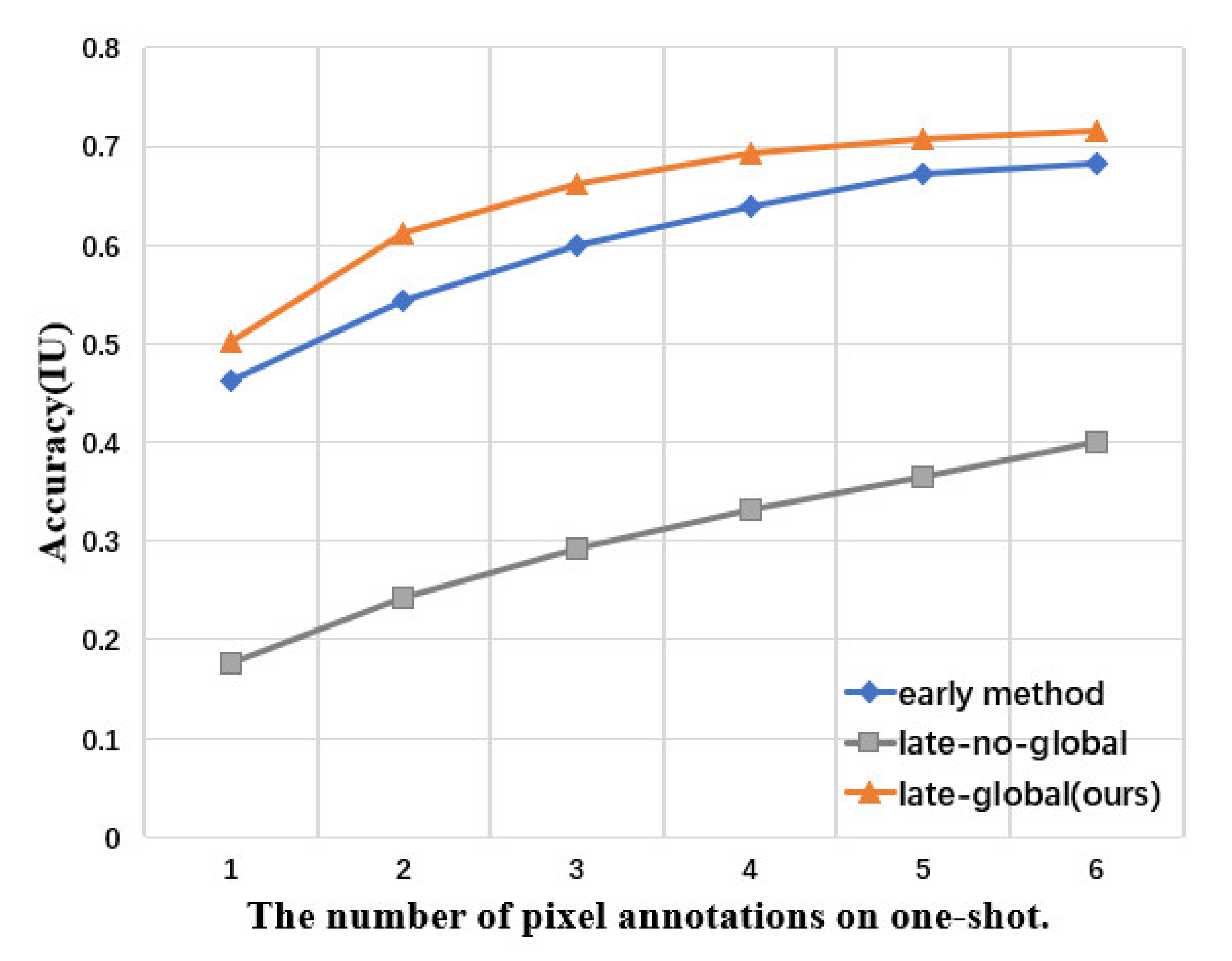
As mentioned in the previous section, we restore the issue as a special case of few-shot segmentation when the support and query images are the same. We mainly compare our methods with Xu et al. [21], because it is state-of-the-art, and we pay more attention to the efficiency and generality of learning labels. Our methods are different from them in support encoding. They fuse by simply stacking, but our fusion factorizes into images and annotations, and we fuse globally. In contrast, our approach is more accurate, with sparse annotations, and it is faster to update, due to a full forward pass of previous methods (see Figure 8). We decided on late-global guidance throughout.

5.2.2. Semantic Segmentation

Because of the high intra-class variance of each task’s appearance, it is not a simple work to apply few-show learning to semantic segmentation. For this problem, we follow the experimental protocol of Shaban et al. [14] and define four class-wise splits [30]. We set up training set from the whole images including non-held-out classes. It has 21 classes (containing background).

We concentrated on evaluating both dense and sparse annotations of the support with full masks and a single point per positive/negative separately (see

Table 1. Few-shot semantic segmentation evaluation on SBD with the IU (%) metric over binary tasks. As shown in the table, our approach is much better than previous methods. Note that foreground–background (FG–BG) is a strong baseline and rivals fine-tuning.

	Dense		Sparse
Method	1-shot	5-shot	1-shot	5-shot
FG–BG	55.0	-	-	-
Fine-tuning	55.1	55.6	-	-
Xu et al.	54.5	57.3	50.8	52.6
Shaban et al.	61.3	61.5	52.5	52.9
Ours	62.2	65.2	59.4	64.8

). We achieved state-of-the-art results on both dense and sparse with just two annotated pixels. The early method of Shaban et al. [14] is incompatible with missing annotations, regrettably, and so is Xu et al. [21]. They are just defined for binary annotation.

In the semantic segmentation problem, we also found a strange phenomenon: Our method is not sensitive to the number of annotations. As shown in

Table 2. Our method is strangely insensitive to the amount of annotations in semantic segmentation. It improves the accuracy of IU (%) very little.

(K,P)-Shot	Accuracy (IU)
(1,1)-shot	59.4
(1,2)-shot	61.3
(1,3)-shot	61.6
(1,4)-shot	61.9
(1,5)-shot	62.1
(1,6)-shot	62.2

, the IU accuracy increases very slowly and inconspicuously by increasing the number of annotations. Basically, this is because one-shot cannot cover all the visual variation in a category. Think about it in terms of segmenting a black long-haired dog, and the guidance information given is obtained from a white short-haired dog. The color and shape between the two are quite different, resulting in inaccurate guidance information. We took another way of thinking and considered solving this problem by increasing one-shot to few-shot. We increased the one-shot to five-shot, while keeping two annotated pixels (one positive pixel and one negative pixel) unchanged, and found that the accuracy of IU increased by about 6%. This is a big promotion.

At the end of the experiment, we put the interactive segmentation and few-shot semantic segmentation together and compared their methods with the four metrics mentioned above. We report the evaluation results in

Table 3. Evaluation results under the settings of (1,3)-shot. For interactive segmentation, our interactive-late-global has a significant improvement in all four metrics, especially in IU. For semantic segmentation, our approach also has about 10% improvement in IU.

	PA	MPA	IU	FWIU
Interactive-early	90.7	69.4	60.0	83.4
Interactive-late-no-global	79.9	39.4	29.3	67.6
Interactive-late-global (ours)	91.0	84.9	66.2	84.6
Semantic-early	88.2	58.1	51.2	79.2
Semantic-late (ours)	91.5	70.9	61.6	84.8

Notes: PA, pixel accuracy; MPA, mean pixel accuracy; FWIU, frequency weighted intersection-over-union.

. Our method achieved the best results for semantic segmentation and interactive segmentation. Then we incorporated the fully connected CRF to our model, respectively, which produced a significant performance boost, about 4% improvement, as shown in

Table 4. Performance of our proposed model with the IU(%) metric before and after CRF. About 4% improvement after CRF.

Method	Before CRF	After CRF
Interactive-late-global (ours)	66.2	69.9
Semantic-late (ours)	61.6	65.4

.

6. Discussion

Our work combines few-shot segmentation with the fully connected CRF to solve the problem of image segmentation under low data settings, producing accurate segmentation predictions and recovering object boundaries as much as possible. At the same time, it keeps a high computing efficiency. The specific method of few-shot segmentation is as follows. Few-shot-guided networks extract the latent task representation from any amount of supervision given of support for interactive inference. Once learned, it can segment new inputs without the supervisor, while maintaining its accuracy and high efficiency. Our experimental results show that the proposed method achieves a good result in the augmented PASCAL VOC 2012 image segmentation dataset, the so-called SBD.

Although we have achieved good results by integrating into our networks the fully connected CRF, there are also some unavoidable limitations. For example, our model is not an end-to-end system. It is just that CRF uses the results of few-shot networks as unary potential function. Therefore, we plan to entirely integrate its two major parts (few-shot networks and fully connected CRFs) and train the whole system in an end-to-end fashion. In addition, we intend to experiment with more datasets. We think this is an area full of challenges, and we hope to make continuous improvement in our future work.

References

- Lake, B.M.; Salakhutdinov, R.; Gross, J.; Tenenbaum, J. One shot learning of simple visual concepts. In Proceedings of the Annual Meeting of the Cognitive Science Society, Boston, MA, USA, 20–23 July 2011; Volume 33. [Google Scholar]
- Lake, B.M.; Salakhutdinov, R.; Tenenbaum, J. One-shot learning by inverting a compositional causal process. In Proceedings of the Advance in Neural Information Processing Systems, Lake Tahoe, NV, USA, 5–10 December 2013; pp. 2526–2534. [Google Scholar]
- Norouzi, M.; Mikolov, T.; Bengio, S.; Singer, Y.; Shlens, J.; Frome, A.; Dean, J. Zero-shot learning by convex combination of semantic embeddings. arXiv 2013, arXiv:1312.5650. [Google Scholar]
- Chen, L.C.; Papandreou, G.; Kokkinos, I.; Murphy, K.; Yuille, A.L. Semantic image segmentation with deep convolutional nets and fully connected CRFs. arXiv 2014, arXiv:1412.7062. [Google Scholar]
- Krahenbuhl, P.; Koltun, V. Efficient inference in fully connected CRFs with gaussian edge potentials. In Proceedings of the Advance in Neural Information Processing Systems, Granada, Spain, 12–15 December 2011; pp. 109–117. [Google Scholar]
- Long, J.; Shelhamer, E.; Darrell, T. Fully convolutional networks for semantic segmentation. In Proceedings of the IEEE Conference on Computer Vision and Pattern Recognition, Boston, MA, USA, 7–12 June 2015; pp. 3431–3440. [Google Scholar]
- Deng, X.; Zheng, Y.; Xu, Y.; Xi, X.; Li, N.; Yin, Y. Graph cut based automatic aorta segmentation with an adaptive smoothness constraint in 3D abdominal CT images. Neurocomputing 2018, 310, 46–58. [Google Scholar] [CrossRef]
- He, K.; Gkioxari, G.; Dollar, P.; Girshick, R. Mask R-CNN. In Proceedings of the IEEE International Conference on Computer Vision, Venice, Italy, 22–29 October 2017; pp. 2961–2969. [Google Scholar]
- Chen, L.-C.; Papandreou, G.; Kokkinos, I.; Murphy, K.; Yuille, A.L. DeepLab: Semantic Image Segmentation with Deep Convolutional Nets, Atrous Convolution, and Fully Connected CRFs. IEEE Trans. Pattern Anal. Mach. Intell. 2018, 40, 834–848. [Google Scholar] [CrossRef] [PubMed]
- Vinyals, O.; Blundell, C.; Lillicrap, T.; Wierstra, D. Matching networks for one shot learning. In Proceedings of the Advance in Neural Information Processing Systems, Barcelona, Spain, 5–10 December 2016; pp. 3630–3638. [Google Scholar]
- Ren, M.; Ravi, S.; Triantafillou, E.; Snell, J.; Swersky, K.; Tenenbaum, L.B.; Zemel, R.S. Meta-learning for semi-supervised few-shot classification. arXiv 2018, arXiv:1803.00676. [Google Scholar]
- Kang, B.; Liu, Z.; Wang, X.; Yu, F.; Feng, J.; Darrell, T. Few-shot object detection via feature reweighting. In Proceedings of the IEEE International Conference on Computer Vision, Seoul, Korea, 27 October–2 November 2019; pp. 8420–8429. [Google Scholar]
- Yan, L.; Zheng, Y.; Cao, J. Few-shot learning for short text classification. Multimedia Tools Appl. 2018, 77, 29799–29810. [Google Scholar] [CrossRef]
- Shaban, A.; Bansal, S.; Liu, Z.; Essa, I.; Boots, B. One-shot learning for semantic segmentation. arXiv 2017, arXiv:1709.03410. [Google Scholar]
- Ravi, S.; Larochelle, H. Optimization as a model for few-shot learning. In Proceedings of the Advance in International Conference on Learning Representations, Chengdu, China, 2–4 June 2017. [Google Scholar]
- Yang, Q.; Chen, W.-N.; Gu, T.; Zhang, H.; Deng, J.D.; Li, Y.; Zhang, J. Segment-Based Predominant Learning Swarm Optimizer for Large-Scale Optimization. IEEE Trans. Cybern. 2016, 47, 2896–2910. [Google Scholar] [CrossRef] [PubMed] [Green Version]
- Rao, D.J.; Mittal, S.; Ritika, S. Siamese neural networks for one-shot detection of railway track switches. arXiv 2017, arXiv:1712.08036. [Google Scholar]
- Chopra, S.; Hadsell, R.; Lecun, Y. Learning a similarity metric discriminatively, with application to face verification. In Proceedings of the IEEE Conference on Computer Vision and Pattern Recognition, San Diego, CA, USA, 20–25 June 2005; Volume 1, pp. 539–546. [Google Scholar]
- Hadsell, R.; Chopra, S.; Lecun, Y. Dimensionality reduction by learning an invariant mapping. In Proceedings of the IEEE Conference on Computer Vision and Pattern Recognition, New York, NY, USA, 17–22 June 2006; Volume 2, pp. 1735–1742. [Google Scholar]
- Snell, J.; Swersky, K.; Zemel, R. Prototypical networks for few-shot learning. In Proceedings of the Advance in Neural Information Processing Systems, Long Beach, CA, USA, 4–9 December 2017; pp. 4077–4087. [Google Scholar]
- Xu, N.; Price, B.; Cohen, S.; Yang, J.; Huang, T.S. Deep interactive object selection. In Proceedings of the IEEE Conference on Computer Vision and Pattern Recognition, Las Vegas, NV, USA, 27–30 June 2016; pp. 373–381. [Google Scholar]
- Kohli, P.; Ladický, L.; Torr, P.H. Robust Higher Order Potentials for Enforcing Label Consistency. Int. J. Comput. Vis. 2009, 82, 302–324. [Google Scholar] [CrossRef] [Green Version]
- Liu, J.; Wang, J.; Fang, T.; Tai, C.L.; Quan, L. Higher-order CRF structural segmentation of 3D reconstructed surfaces. In Proceedings of the IEEE in International Conference on Computer Vision, Santiago, Chile, 7–13 December 2015; pp. 2093–2101. [Google Scholar]
- Chen, L.C.; Papandreou, G.; Schroff, F.; Adam, H. Rethinking atrous convolution for semantic image segmentation. arXiv 2017, arXiv:1706.05587. [Google Scholar]
- Fang, Y.; Zhang, H.; Ren, Y. Graph regularised sparse NMF factorisation for imagery de-noising. IET Comput. Vis. 2018, 12, 466–475. [Google Scholar] [CrossRef]
- Nichol, A.; Achiam, J.; Schulman, J. On first-order meta-learning algorithms. arXiv 2018, arXiv:1803.02999. [Google Scholar]
- Chen, Z.; Zheng, Y.; Li, X.; Luo, R.; Jia, W.; Lian, J.; Li, C. Interactive trimap generation for digital matting based on single-sample learning. Electronics 2020, 9, 659. [Google Scholar] [CrossRef]
- Simonyan, K.; Zisserman, A. Very deep convolutional networks for large-scale image Rrecognition. arXiv 2014, arXiv:1409.1556. [Google Scholar]
- Russakovsky, O.; Deng, J.; Su, H.; Krause, J.; Satheesh, S.; Ma, S.; Huang, Z.; Karpathy, A.; Khosla, A.; Bernstein, M.; et al. ImageNet Large Scale Visual Recognition Challenge. Int. J. Comput. Vis. 2015, 115, 211–252. [Google Scholar] [CrossRef] [Green Version]
- Rakelly, K.; Shelhamer, E.; Darrell, T.; Efros, A.A.; Levine, S. Few-shot segmentation propagation with guided networks. arXiv 2018, arXiv:1806.07373. [Google Scholar]
- Rakelly, K.; Shelhamer, E.; Darrell, T.; Efros, A.A.; Levine, S. Conditional networks for few-shot semantic segmentation. In Proceedings of the International Conference on Learning Representations Workshop, Vancouver, BC, Canada, 30 April–3 May 2018. [Google Scholar]
- Yoon, J.S.; Rameau, F.; Kim, J.; Lee, S.; Shin, S.; Kweon, I. Pixel-level matching for video object segmentation using convolutional neural networks. In Proceedings of the IEEE International Conference on Computer Vision, Venice, Italy, 22–29 October 2017; pp. 2167–2176. [Google Scholar]
- Eigen, D.; Fergus, R. Predicting depth, Surface normals and semantic labels with a common multi-scale convolutional architecture. In Proceedings of the IEEE International Conference on Computer Vision, Santiago, Chile, 7–13 December 2015; pp. 2650–2658. [Google Scholar]
- Mostajabi, M.; Yadollahpour, P.; Shakhnarovich, G. Feedforward semantic segmentation with zoom-out features. In Proceedings of the IEEE Conference on Computer Vision and Pattern Recognition, Boston, MA, USA, 7–12 June 2015; pp. 3376–3385. [Google Scholar]
- Rother, C.; Kolmogorov, V.; Blake, A. “GrabCut”: Interactive foreground extraction using iterated graph cuts. ACM Trans. Graph. 2012, 23, 309–314. [Google Scholar] [CrossRef]
- Shotton, J.; Winn, J.; Rother, C.; Criminisi, A. TextonBoost for Image Understanding: Multi-Class Object Recognition and Segmentation by Jointly Modeling Texture, Layout, and Context. Int. J. Comput. Vis. 2007, 81, 2–23. [Google Scholar] [CrossRef] [Green Version]
- Hariharan, B.; Arbelaez, P.; Bourdev, L.; Maji, S.; Malik, J. Semantic contours from inverse detectors. In Proceedings of the IEEE International Conference on Computer Vision, Barcelona, Spain, 6–13 November 2011; pp. 991–998. [Google Scholar]
- Caelles, S.; Maninis, K.; Ponttuset, J.; Cremers, D.; Van Gool, L. One-shot video object segmentation. In Proceedings of the IEEE Conference on Computer Vision and Pattern Recognition, Honolulu, HI, USA, 21–26 July 2017; pp. 221–230. [Google Scholar]
- Badrinarayanan, V.; Badrinarayanan, V.; Cipolla, R. SegNet: A Deep Convolutional Encoder-Decoder Architecture for Image Segmentation. IEEE Trans. Pattern Anal. Mach. Intell. 2017, 39, 2481–2495. [Google Scholar] [CrossRef] [PubMed]
Figure 1.
Proposed model overview. See
Section 4 for details.
Figure 2.
Our few-shot image segmentation subsumes semantic and interactive. It is worth noting that interactive-based cannot propagate annotations across different images. Our proposed method can be used in both cases.
Figure 3.
Extracting a task representation from the support. (a) Previous work simply stack the support and annotations channel-wise. (b) Our method factorizes into image and annotations streams and improves learning efficiency and inference accuracy.
Figure 4.
Globalizing the task representation propagation: In this example, we annotate a single dog (b) on the image (a), but global guidance causes all similar dogs to be segmented (d) instead of segmenting an annotated dog (c).
Figure 5.
Illustration of the segmentation branch. This part describes the fusion of the task representation with the query features and generates rough prediction results.
Figure 6.
Comparison of segmentation effect. (a) The original image. (b) The ground truth of the image. (c) The segmentation result after few-shot guided network. (d) The final output after the fully connected conditional random field (CRF) optimization.
Figure 7.
Visualization results on Semantic Boundaries Dataset (SBD)-val. For each row, we show the query image, the segmentation result delivered by the few-shot guided network, and the refined segmentation result of the fully connected CRF. The last row shows failure modes.
Figure 8.
Interactive segmentation of objects in the support. The experimental results show that the accuracy of intersection-over-union (IU) is not significantly improved when the number of annotated pixels is more than five.