Does Deep Learning Work Well for Categorical Datasets with Mainly Nominal Attributes?

Abstract

Given the complexity of real-world datasets, it is difficult to present data structures using existing deep learning (DL) models. Most research to date has concentrated on datasets with only one type of attribute: categorical or numerical. Categorical data are common in datasets such as the German (-categorical) credit scoring dataset, which contains numerical, ordinal, and nominal attributes. The heterogeneous structure of this dataset makes very high accuracy difficult to achieve. DL-based methods have achieved high accuracy (99.68%) for the Wisconsin Breast Cancer Dataset, whereas DL-inspired methods have achieved high accuracy (97.39%) for the Australian credit dataset. However, to our knowledge, no such method has been proposed to classify the German credit dataset. This study aimed to provide new insights into the reasons why DL-based and DL-inspired classifiers do not work well for categorical datasets, mainly consisting of nominal attributes. We also discuss the problems associated with using nominal attributes to design high-performance classifiers. Considering the expanded utility of DL, this study's findings should aid in the development of a new type of DL that can handle categorical datasets consisting of mainly nominal attributes, which are commonly used in risk evaluation, finance, banking, and marketing.

1. Introduction

1.1. Background

Among existing deep learning (DL) models, convolutional neural networks (CNNs) [1,2] are the best architecture for most tasks involving image recognition, classification, and detection [3]. However, Wolpert [4,5] described what has come to be known as the no free lunch (NFL) theorem, which implies that all learning algorithms perform equally well when averaged over all possible datasets. This counterintuitive concept thereby suggests the infeasibility of finding a general, highly predictive algorithm. Gŏmez and Rojas [6] subsequently empirically investigated the effects of the NFL theorem on several popular machine learning (ML) classification techniques using real-world datasets.

1.2. Types of Data Attributes

It is substantially more challenging to accurately present data structures using existing DL models due to the complexity and variety of real-world datasets. Most of the research on this issue has concentrated on datasets with only one attribute: categorical or numerical. However, the number of cases with more than one type of attribute in a supervised control architecture has increased [7]. Categorical attributes are composed of two subclasses—nominal and ordinal—with the latter inheriting some properties of the former. Similar to nominal attributes, all of the categories (i.e., possible values) of the attributes in ordinal data—in other words, the data associated with only the ordinal attributes—are qualitative and therefore unsuitable for mathematical operations; however, they are naturally ordered and comparable [8]. As an example, consider a dataset related to individuals containing a numerical attribute such as 0.123, 4.56, 10, 100, an ordinal attribute such as a Stage I, II, or III cancer diagnosis, and a nominal attribute such as university student, public employee, company employee, physician, or professor [9].

1.3. Heterogeneous Datasets

A numerical dataset’s characteristics differ from those of categorical datasets that contain only ordinal attributes, such as the Wisconsin Breast Cancer Dataset (WBCD). (https://archive.ics.uci.edu/ml/datasets/breast+cancer+wisconsin+(original)). From a practical perspective, categorical data that involve a mix of nominal and ordinal attributes are common in credit scoring datasets [10]. The German (-categorical) credit scoring dataset (https://archive.ics.uci.edu/mL/datasets/statlog+(german+credit+data)) is a typical heterogeneous dataset that contains numerical, ordinal, and nominal attributes. The heterogeneous structure of this dataset makes very high accuracy difficult to achieve. Several alternative approaches, such as artificial bee colony (ABC)-based support vector machines (SVMs) [11], feature selection and random forest (RF) [12], Information Gain Directed Feature Selection [13], synthetic minority oversampling technique (SMOTE)-based ensemble classification [14], and extreme learning machines (ELMs) [15], have been developed in recent years for the German credit dataset.

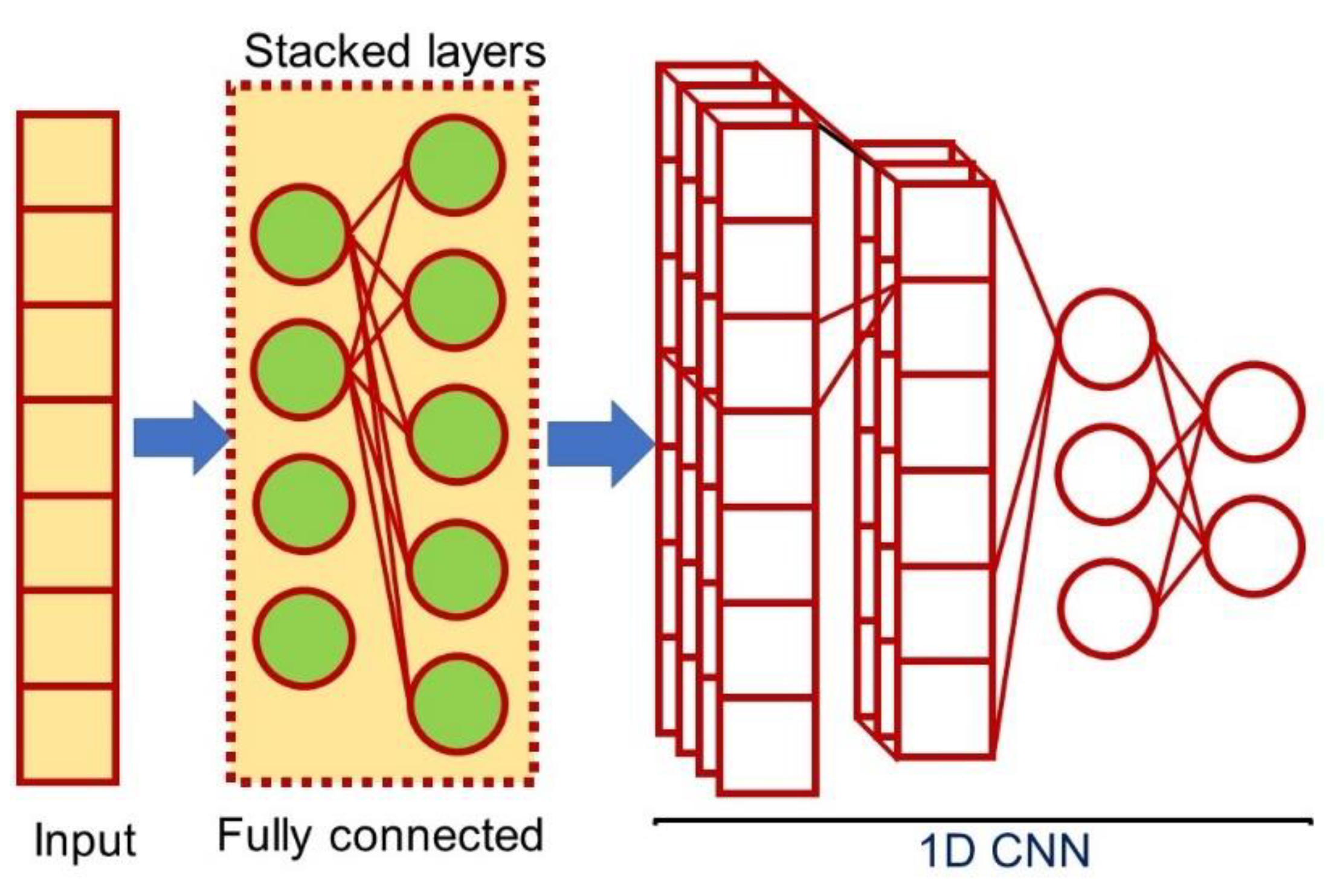
1.4. Deep Learning (DL) Approaches for Datasets with Ordinal Attributes

The present author previously proposed a general-purpose and straightforward method [16] to map weights in deep neural networks (DNNs) trained by deep belief networks (DBNs [17]) to weights in backpropagation neural networks (NNs). It uses the recursive-rule eXtraction (Re-RX [18]) algorithm with J48graft [19,20], which led to the proposal of a new method to extract accurate and interpretable classification rules for categorical datasets, including rating or grading ordinal attributes. This method was then applied to the WBCD, a small, high-abstraction ordinal dataset with prior knowledge [21]. The present author also noted that the German credit dataset was a relatively low-level abstraction dataset that mainly includes the nominal attributes of banking professionals without prior knowledge.

1.5. State-of-the-Art DL Classifiers for Categorical and Mixed Datasets

A variety of high-accuracy classifiers have recently been proposed. DL-based methods used for the WBCD have achieved accuracy as high as 99.68% [22,23,24], whereas DL-inspired methods used for the Australian credit dataset (http://archive.ics.uci.edu/ml/datasets/statlog+(australian+credit+approval)) have achieved accuracy as high as 97.39% [24,25].

Recently, the present author presented a new rule extraction method [26] for achieving transparency and conciseness in credit scoring datasets with heterogeneous attributes using a one-dimensional (1D) fully-connected layer first (FCLF)-CNN [23] combined with the Re-RX algorithm with a J48graft decision tree (hereafter 1D FCLF-CNN [Figure 1]). Although it does not completely overcome the accuracy–interpretability dilemma for DL, it does appear to resolve this issue for credit scoring datasets with heterogeneous attributes.

1.6. Novelty of This Paper

Nevertheless, and contrary to our expectation, although it appears relatively easy to construct DL-based and DL-inspired classifiers with very high accuracies, to our knowledge, no method has been proposed to classify the German credit dataset. We hypothesized that one reason for the high accuracies would be the ratio of the number of ordinal and nominal attributes.

In this paper, we provide new insights for the reasons why DL-based and DL-inspired classifiers do not work well for categorical datasets mainly consisting of nominal attributes, as well as the barriers to achieving very high accuracies for such datasets. We also discuss the pitfalls of using nominal attributes to design high-performance classifiers.

2. Categorical Datasets and Their Recent High Accuracies

In this section, we first tabulate the characteristics of three categorical datasets (

Table 1. Characteristics of the Wisconsin Breast Cancer Dataset (WBCD), German, and Australian datasets.

Dataset	# Instances	# Total Features	Categorical Nominal	Categorical Ordinal	Numerical
WBCD	699	9	0	9	0
German	1000	20	10	3	7
Australian	690	14	0	8	6

).

Table 2. Comparisons of recent classifier performances for the Wisconsin Breast Cancer Dataset (WBCD).

Method	TS ACC (%)	AUC-ROC	Year
Fuzzy-rough nearest neighbor with instance feature selection [10CV] [33]	99.71	1.000	2015
DBN-NN [22]	99.68	----	2016
Particle Swarm Optimization (PSO)_SVM [10CV] [34]	99.30	0.993	2012
Genetically Optimized Neural Network (GONN) [10CV] [35]	99.26	1.000	2015
Gauss-Newton Representation-based Algorithm [10CV] [36]	99.23	0.997	2017
C-MLP2LN [10CV] [37]	99.00	----	2000
Ensemble of 1D FCLF-CNN [10CV] [23]	98.71	----	2018
Deep neural network (DNN) and recursive feature elimination (RFE) [80:20 split] [24]	98.62	----	2018
Bio-inspired weighted quantum swarm optimization and SVM ensemble [10CV] [38]	98.70	----	2019
Deep Forest [10CV] [31,32]	95.52 1	----	2020

¹ We investigated the WBCD using Zhou and Feng’s codes. “----“means that the literature provided no information about the area under the receiver operating characteristic curve (AUC-ROC); TS ACC: accuracy for test dataset; SVM: support vector machine; 10CV: 10-fold cross-validation; 1D FCLF-CNN: one-dimensional fully-connected layer first convolutional neural network.

and

Table 3. Comparison of recent classifier performances for the German dataset.

Method	TS ACC (%)	AUC-ROC (%)	Year
Neighborhood rough set + multi-layer ensemble classification [10CV] [10]	86.57	----	2018
Artificial bee-colony based SVM [10CV] [11]	84.00	----	2018
Bolasso based feature selection + random forest [10CV] [12]	84.00	0.713	2020
Information Gain Directed Feature Selection algorithm [10CV] [13]	82.80	0.753	2018
SMOTE-based ensemble method [10CV] [14]	78.70	0.810	2019
Extreme Learning Machine [10CV] [15]	76.40	0.801	2017
1D FCLF-CNN [10CV] [23]	74.70 2 [25]	0.697 2 [25]	2018
Deep Forest [10CV] [31,32]	71.12 1	----	2017

¹ We investigated the German dataset [25] using Zhou and Feng’s codes [31]. ² We implemented the program for the German dataset based on Liu et al.’s method. “----“ means that the literature provided no information about the area under the receiver operating characteristic curve (AUC-ROC); TS ACC: accuracy for test dataset; SVM: support vector machine; 10CV: 10-fold cross-validation; 1D FCLF-CNN: one-dimensional fully-connected layer first convolutional neural network.

show the test accuracies and area under the receiver operating characteristic curves (AUC-ROCs) [27] obtained by recent high accuracy classifiers for the WBCD, and the German dataset. A new method of concordant partial AUC (cpAUC) [28] was proposed as a related reference.

Table 4. Parameter settings for training the 1D FCLF-CNN for the German and Australian credit scoring datasets.

Dataset	German	Australian
Pruning stop rate for 1D FCLF-CNN	0.13	0.20
# of first layer hidden units for 1D FCLF-CNN	4	3
Learning rate for 1D FCLF-CNN	0.0182	0.0106
Momentum factor for 1D FCLF-CNN	0.1154	0.7549
# of filters in each branch in the inception module	19	8
# of channels after concatenation	57	24

shows parameter settings for training the 1D FCLF-CNN for the German and Australian credit scoring datasets.

Table 5. Comparison of recent classifier performances for the Australian dataset.

Method	TS ACC (%)	AUC-ROC (%)	Year
Deep Genetic Cascade Ensemble of SVM classifier [10CV] [25]	97.39	----	2019
Spiking extreme learning machine [10CV] [40]	95.98	0.970	2019
Artificial bee colony-based SVM [10CV] [11]	92.75	----	2018
Ensemble feature selection + multilayer ensemble classification [100 × 10CV] [39]	92.69	----	2019
DNN (sequential neural network, convolution neural network) [10CV] [41]	87.54	----	2019
1D FCLF-CNN [10CV] [23]	85.80 1 [25]	0.859 [25]	2018

¹ We implemented the Australian dataset program [25] based on the Liu et al. method. “----“means that the literature provided no information about the area under the receiver operating characteristic curve (AUC-ROC); TS ACC: accuracy for test dataset; SVM: support vector machine; 10CV: 10-fold cross-validation; 1D FCLF-CNN: one-dimensional fully-connected layer first convolutional neural network.

also shows the test accuracies and AUC-ROCs obtained by recent high accuracy classifiers for the Australian dataset.

2.1. The Wisconsin Breast Cancer Dataset (WBCD) and Classification Accuracies

2.1.1. The Wisconsin Breast Cancer Dataset (WBCD)

The WBCD is composed of 699 samples (16 with missing values) obtained from fine-needle aspiration (FNA) [29] of human breast tissue. FNA allows malignancy in breast masses to be investigated in a noninvasive and cost-effective manner. In total, nine features related to the size, shape, and texture of the cell nuclei are measured in each sample. The observed values are scored on a 10-point scale, where 1 denotes the closest to being benign, and each sample is given a class label (benign or malignant). Among the 683 complete samples, 339 malignant and 444 benign cases were observed. Pathologists assessed the features based on an analysis of these nine ordinal features [30].

2.1.2. Recent High Accuracies by Classifiers for the WBCD

The accuracy for the WBCD plateaus at around 99.00%. DL-based classifiers [22,23,24] are relatively competitive with other recent high-accuracy classifiers; however, Deep Forest does not work well for the WBCD. Zhou and Feng [31,32] proposed a unique gcForest (multi-grained cascade forest) approach for constructing a non-NN-style deep model. Their approach was a novel decision tree ensemble with a cascade structure that enables representation learning. We first demonstrated that this DL-inspired method had a considerably lower classification accuracy of 95.52%.

2.2. Credit Scoring Datasets

Credit application scoring is an effective method for classifying whether a credit applicant belongs to a legitimate (creditworthy) or suspicious (non-creditworthy) group based on their credentials. Improving the predictive performance of credit scoring models, especially for applicants that fall into the non-creditworthy group, could be expected to have a substantial impact on the financial industry [38].

2.2.1. German (-Categorical) Dataset

The German dataset contains 1000 samples with 20 features that describe the applicant’s credit history. In this dataset, 700 and 300 samples describe creditworthy and uncreditworthy applicants, respectively. Nominal attributes include the status of an existing checking account, credit history, the purpose of credit taken by a customer, savings accounts/bonds, present type and length of employment, personal characteristics and sex, debtors or guarantors, property holdings, installment plans, housing status, and job status [39].

2.2.2. Recent High-Accuracy Classifiers for the German Dataset

In many cases, credit scoring datasets contain customer profiles that consist of numerical, ordinal, and mainly nominal attributes; here, these are referred to as heterogeneous credit scoring datasets [26]. This section on the German dataset reveals the pros and cons of DL, DL-based classifiers, and DL-inspired classifiers from different perspectives. Ensemble classifiers with a neighborhood rough set [10], ABC-based SVM [11], and Bolasso based feature selection and RF [12] showed very high accuracies.

We used the parameter settings shown in Table 4 for training the 1D FCLF-CNN for the German and Australian credit scoring datasets.

2.2.3. Australian Dataset

The Australian dataset consists of 690 samples with 14 features. Each sample in the Australian dataset is composed of six categorical and eight numerical attributes, as well as a class attribute (accepted as positive or rejected as negative), where 307 and 383 instances are positive and negative applicants, respectively. The Australian dataset consists of credit card applications, but the feature values and names are changed into random symbols to preserve the data’s secrecy [39].

3. Discussion

3.1. Discussion

We hypothesized that a reason why DL does not work well was the number of features and the characteristics of the attributes. At first glance, the results in Table 3 seemed to be following their descriptions of low-dimensional data for Deep Forest [31,32]. The authors noted that “fancy architectures like CNNs could not work on such data as there are too few features without spatial relationships” [32] (p. 81) because a DL-based classifier [23] achieved an accuracy of 98.71%, which made it easy to classify the WBCD with only nine ordinal attributes.

However, a DL-based classifier [23,41] and Deep Forest [31,32] ranked at the bottom (Table 3 and Table 5). Deep Forest showed the lowest classification accuracy, at 71.12%. Differences in the accuracies obtained using a 1D FCLF-CNN combined with Re-RX with J48graft (1D FCLF-CNN with Re-RX with J48graft) and Deep Forest were 10.17% and 15.45%, respectively, with the highest accuracy of 86.57% [10]. These accuracies were inferior to that of the highest obtained using a rule extraction method (79.0%) [42].

We believe that the main reason for this is that the German dataset consists of mainly nominal attributes, which are commonly found in finance and banking, risk evaluation [12], and marketing [43]. Therefore, innovations are needed for DL, DL-based, and DL-inspired methods for heterogeneous datasets such as the German credit dataset. We also argue that the Bene1 [44] and Bene2 [44] datasets, which have been used by major Benelux-based financial institutions to summarize consumer credit data, consist of mainly nominal attributes.

Surprisingly, a new deep genetic cascade ensemble of different SVM classifiers (so-called Deep Genetic Cascade Ensembles of Classifiers [DGCEC]) system [25] achieved the current highest accuracy (97.39%) for the Australian dataset. That study aimed to design a novel deep genetic cascade ensemble (16-layer system) of SVM classifiers based on evolutionary computation, ensemble learning, and DL techniques that would allow the effective binary classification of accepted or rejected borrowers. This new method was based on a combination of the following: SVM classifiers, normalizations, feature extractions, kernel functions, parameter optimization, ensemble learning, DL, layered learning, supervised training, feature selection (attributes), and the optimization of classifier parameters using a genetic algorithm.

Although the spiking extreme learning machine method [39] was very systematic and sophisticated for the Australian dataset, it achieved the second-highest accuracy (95.98%) DL-inspired tactic can achieve considerably higher classification accuracies. This method was specialized to predict creditworthiness in the Australian dataset. Hence, the results obtained by these methods are worse than those obtained by the DGCEC system.

3.2. A Black-Box ML Approach to Achieve Very High Accuracies for the German (-Numerical) Credit Dataset

Pławiak et al. [45] recently proposed the Deep Genetic Hierarchical Network of Learners, a fusion-based system with a 29-layer structure that includes ML algorithms, SVM algorithms, k-nearest neighbors, and probabilistic NNs, as well as a fuzzy system, normalization techniques, feature extraction approaches, kernel functions, and parameter optimization techniques based on error calculation. Remarkably, they achieved the highest accuracy (94.60%) for a German (-numerical; 24 attributes) dataset with all numerical and no nominal attributes. However, this dataset had no nominal attributes, making it easy to classify, and thus, fundamentally different from the German (-categorical; 20 attributes) dataset. As a result, we omitted the performance from Table 3. Furthermore, even if this kind of ML technique is effective to enhance classification accuracy, these methods hinder the conversion of a “black box” DNN trained by DL into a “white box” consisting of a series of interpretable classification rules [46].

3.3. Pitfalls for Handling Nominal Attributes to Design High-performance Classifiers

As shown in Table 1, the WBCD consists of ordinal attributes. The Australian dataset is a mixed dataset, i.e., it consists of ordinal and numerical attributes. On the other hand, the German credit dataset is a mixed dataset that consists of mainly nominal attributes. When attempting to achieve only the highest accuracy for the German dataset, many papers often do not focus on handling the datasets with heterogeneous attributes and maintaining the characteristics of the nominal attributes appropriately. For example, the highest accuracy achieved for the German (-categorical) dataset was 86.57% by Tripathi et al. [10]. Kuppili et al. [40] and Tripathi et al. [39] achieved considerably higher accuracies for the German dataset using an SVM and NN requiring that each data instance be represented as a vector of real numbers. However, they did not appropriately handle nominal attributes as they converted them into numerical attributes before feeding them into the classifiers. If this pitfall can be avoided, classifiers with much higher accuracy can be designed using DL-based or DL-inspired methods.

4. Conclusions

In this paper, we have provided new insights into why DL-based and DL-inspired classifiers do not work well for categorical datasets that mainly consist of nominal attributes and the barriers to achieving very high accuracies for such datasets. One limitation of this work is the limited number of categorical datasets with mainly nominal attributes. As mentioned above, there are bigger datasets similar to the German datasets, including the Bene1, Bene2, Lending Club, and Bank Loan Status datasets. Considering the vastly expanded utility of DL, attempts should be made to develop a new type of DL to handle categorical datasets consisting of mainly nominal attributes, commonly used in risk evaluation, finance, banking, and marketing.

References

1. LeCun, Y.; Boser, B.; Denker, J.S.; Henderson, D.; Howard, R.E.; Hubbard, W.; Jackel, L.D. Handwritten digit recognition with a back-propagation network. In Advances in Neural Information Processing Systems 2; Touretzky, D.S., Ed.; MIT Press: Cambridge, MA, USA, 1989; pp. 396–404. [Google Scholar]
2. LeCun, Y.; Boser, B.; Denker, J.S.; Henderson, D.; Howard, R.E.; Hubbard, W.; Jackel, L.D. Backpropagation applied to handwritten zip code recognition. Neural Comput. 1989, 1, 541–551. [Google Scholar] [CrossRef]
3. LeCun, Y.; Bengio, Y.; Hinton, G. Deep learning. Nature 2015, 521, 436–444. [Google Scholar] [CrossRef]
4. Wolpert, D. Stacked generalization. Neural Netw. 1992, 5, 241–259. [Google Scholar] [CrossRef]
5. Wolpert, D.H. The existence of a prior distinctions between learning algorithms. Neural Comput. 1996, 8, 1391–1420. [Google Scholar] [CrossRef]
6. Gŏmez, D.; Rojas, A. An empirical overview of the no free lunch theorem and its effect on real-world machine learning classification. Neural Comput. 2016, 28, 216–228. [Google Scholar] [CrossRef] [PubMed] [Green Version]
7. Liang, Q.; Wang, K. Distributed outlier detection in hierarchically structured datasets with mixed attributes. Qual. Technol. Quant. Manag. 2019, 17, 337–353. [Google Scholar] [CrossRef]
8. Domingo-Ferrer, J.; Solanas, A. A measure of variance for hierarchical nominal attributes. Inf. Sci. 2008, 178, 4644–4655. [Google Scholar] [CrossRef]
9. Zhang, Y.; Cheung, Y.-M.; Tan, K.C. A Unified Entropy-Based Distance Metric for Ordinal-and-Nominal-Attribute Data Clustering. IEEE Trans. Neural Networks Learn. Syst. 2020, 31, 39–52. [Google Scholar] [CrossRef]
10. Tripathi, D.; Edla, D.R.; Cheruku, R. Hybrid credit scoring model using neighborhood rough set and multi-layer ensemble classification. J. Intell. Fuzzy Syst. 2018, 34, 1543–1549. [Google Scholar] [CrossRef]
11. Hsu, F.-J.; Chen, M.-Y.; Chen, Y.-C. The human-like intelligence with bio-inspired computing approach for credit ratings prediction. Neurocomputing 2018, 279, 11–18. [Google Scholar] [CrossRef]
12. Arora, N.; Kaur, P.D. A Bolasso based consistent feature selection enabled random forest classification algorithm: An application to credit risk assessment. Appl. Soft Comput. 2020, 86, 105936. [Google Scholar] [CrossRef]
13. Jadhav, S.; He, H.; Jenkins, K. Information gain directed genetic algorithm wrapper feature selection for credit rating. Appl. Soft Comput. 2018, 69, 541–553. [Google Scholar] [CrossRef] [Green Version]
14. Shen, F.; Zhao, X.; Li, Z.; Li, K.; Meng, Z. A novel ensemble classification model based on neural networks and a classifier optimisation technique for imbalanced credit risk evaluation. Phys. A: Stat. Mech. Its Appl. 2019, 526, 121073. [Google Scholar] [CrossRef]
15. Bequé, A.; Lessmann, S. Extreme learning machines for credit scoring: An empirical evaluation. Expert Syst. Appl. 2017, 86, 42–53. [Google Scholar] [CrossRef]
16. Hayashi, Y. Use of a Deep Belief Network for Small High-Level Abstraction Data Sets Using Artificial Intelligence with Rule Extraction. Neural Comput. 2018, 30, 3309–3326. [Google Scholar] [CrossRef] [PubMed]
17. Hinton, G.E.; Salakhutdinov, R.R. Reducing the Dimensionality of Data with Neural Networks. Science 2006, 313, 504–507. [Google Scholar] [CrossRef] [PubMed] [Green Version]
18. Setiono, R.; Baesens, B.; Mues, C. Recursive Neural Network Rule Extraction for Data with Mixed Attributes. IEEE Trans. Neural Networks 2008, 19, 299–307. [Google Scholar] [CrossRef]
19. Hayashi, Y.; Nakano, S. Use of a recursive-rule extraction algorithm with J48graft to archive highly accurate and concise rule extraction from a large breast cancer dataset. Inform. Med. Unlocked 2015, 1, 9–16. [Google Scholar] [CrossRef] [Green Version]
20. Webb, G.I. Decision tree grafting from the all-tests-but-one partition. In Proceedings of the 16th International Joint Conference on Artificial Intelligence; Morgan Kaufmann, San Mateo, CA, USA; 1999; pp. 702–707. [Google Scholar]
21. Gűlçehre, C.; Bengio, Y. Knowledge matters: Importance of prior information for optimization. J. Mach. Learn. Res. 2016, 17, 1–32. [Google Scholar]
22. Abdel-Zaher, A.M.; Eldeib, A.M. Breast cancer classification using deep belief networks. Expert Syst. Appl. 2016, 46, 139–144. [Google Scholar] [CrossRef]
23. Liu, K.; Kang, G.; Zhang, N.; Hou, B. Breast Cancer Classification Based on Fully-Connected Layer First Convolutional Neural Networks. IEEE Access 2018, 6, 23722–23732. [Google Scholar] [CrossRef]
24. Karthik, S.; Perumal, R.S.; Mouli, P.V.S.S.R.C. Breast Cancer Classification Using Deep Neural Networks. In Knowledge Computing and Its Applications; Anouncia, S.M., Wiil, U.K., Eds.; Springer: New York, NY, USA, 2018; pp. 227–241. [Google Scholar]
25. Pławiak, P.; Abdar, M.; Acharya, U.R. Application of new deep genetic cascade ensemble of SVM classifiers to predict the Australian credit scoring. Appl. Soft Comput. 2019, 84, 105740. [Google Scholar] [CrossRef]
26. Hayashi, Y.; Takano, N. One-Dimensional Convolutional Neural Networks with Feature Selection for Highly Concise Rule Extraction from Credit Scoring Datasets with Heterogeneous Attributes. Electronics 2020, 9, 1318. [Google Scholar] [CrossRef]
27. Salzberg, S.L. On Comparing Classifiers: Pitfalls to Avoid and a Recommended Approach. Data Min. Knowl. Discov. 1997, 1, 317–328. [Google Scholar] [CrossRef]
28. Carrington, A.; Fieguth, P.W.; Qazi, H.; Holzinger, A.; Chen, H.; Mayr, F.; Douglas, G.; Manuel, D. A new concordant partial AUC and partial c statistic for imbalanced data in the evaluation of machine learning algorithms. BMC Med Informatics Decis. Mak. 2020, 20, 4–12. [Google Scholar] [CrossRef]
29. Manfrin, E.; Mariotto, R.; Remo, A.; Reghellin, D.; Dalfior, D.; Falsirollo, F.; Bonetti, F. Is there still a role for fine-needle aspiration cytology in breast cancer screening? Cancer 2008, 114, 74–82. [Google Scholar] [CrossRef]
30. Fogliatto, F.S.; Anzanello, M.J.; Soares, F.; Brust-Renck, P.G. Decision Support for Breast Cancer Detection: Classification Improvement Through Feature Selection. Cancer Control. 2019, 26, 1–8. [Google Scholar] [CrossRef]
31. Zhou, Z.-H.; Feng, J. Deep forest: Towards an alternative to deep neural networks. In Proceedings of the 26th International Joint Conference on Artificial Intelligence, Melbourne, Australia, 19–25 August 2017; pp. 3553–3559. [Google Scholar]
32. Zhou, Z.-H.; Feng, J. Deep forest. Natl. Sci. Rev. 2019, 6, 74–86. [Google Scholar] [CrossRef]
33. Onan, A. A fuzzy-rough nearest neighbor classifier combined with consistency-based subset evaluation and instance selection for automated diagnosis of breast cancer. Expert Syst. Appl. 2015, 42, 6844–6852. [Google Scholar] [CrossRef]
34. Chen, H.-L.; Yang, B.; Wang, G.; Wang, S.-J.; Liu, J.; Liu, D.-Y. Support Vector Machine Based Diagnostic System for Breast Cancer Using Swarm Intelligence. J. Med Syst. 2012, 36, 2505–2519. [Google Scholar] [CrossRef]
35. Bhardwaj, A.; Tiwari, A. Breast cancer diagnosis using Genetically Optimized Neural Network model. Expert Syst. Appl. 2015, 42, 4611–4620. [Google Scholar] [CrossRef]
36. Dora, L.; Agrawal, S.; Panda, R.; Abraham, A. Optimal breast cancer classification using Gauss–Newton representation based algorithm. Expert Syst. Appl. 2017, 85, 134–145. [Google Scholar] [CrossRef]
37. Duch, W.; Adamczak, R.; Grąbczewski, K.; Jankowski, N. Neural methods of knowledge extraction. Control Cybern. 2000, 29, 997–1017. [Google Scholar]
38. Latchoumi, T.P.; Ezhilarasi, T.P.; Balamurugan, K. Bio-inspired weighed quantum particle swarm optimization and smooth support vector machine ensembles for identification of abnormalities in medical data. SN Appl. Sci. 2019, 1, 1137. [Google Scholar] [CrossRef] [Green Version]
39. Tripathi, D.; Edla, D.R.; Cheruku, R.; Kuppili, V. A novel hybrid credit scoring model based on ensemble feature selection and multilayer ensemble classification. Comput. Intell. 2019, 35, 371–394. [Google Scholar] [CrossRef]
40. Kuppili, V.; Tripathi, D.; Edla, D.R. Credit score classification using spiking extreme learning machine. Comput. Intell. 2020, 36, 402–426. [Google Scholar] [CrossRef]
41. Tai, L.Q.; Vietnam, V.B.A.O.; Huyen, G.T.T. Deep Learning Techniques for Credit Scoring. J. Econ. Bus. Manag. 2019, 7, 93–96. [Google Scholar] [CrossRef]
42. Hayashi, Y.; Oishi, T. High Accuracy-priority Rule Extraction for Reconciling Accuracy and Interpretability in Credit Scoring. New Gener. Comput. 2018, 36, 393–418. [Google Scholar] [CrossRef]
43. Liu, P.J.; McFerran, B.; Haws, K.L. Mindful Matching: Ordinal Versus Nominal Attributes. J. Mark. Res. 2019, 57, 134–155. [Google Scholar] [CrossRef]
44. Baesens, B.; Setiono, R.; Mues, C.; Vanthienen, J. Using Neural Network Rule Extraction and Decision Tables for Credit-Risk Evaluation. Manag. Sci. 2003, 49, 312–329. [Google Scholar] [CrossRef] [Green Version]
45. Pławiak, P.; Abdar, M.; Pławiak, J.; Makarenkov, V.; Acharya, U.R. DGHNL: A new deep genetic hierarchical network of learners for prediction of credit scoring. Inf. Sci. 2020, 516, 401–418. [Google Scholar] [CrossRef]
46. Hayashi, Y. The Right Direction Needed to Develop White-Box Deep Learning in Radiology, Pathology, and Ophthalmology: A Short Review. Front. Robot. AI 2019, 6. [Google Scholar] [CrossRef]
Figure 1. Schematic overview of a one-dimensional fully-connected layer first convolutional neural network (1D FCLF-CNN).
Electronics 09 01966 g001