Simulation of a Smart Sensor Detection Scheme for Wireless Communication Based on Modeling

Abstract

The principle of sensing and sending information applies to all kinds of communications in different media like air, water, etc. During data transmission through sensors, the most important issue is sensing failure problems. In communication systems, sensing failure problems generally occur and affect sensor system performance. In this study, sensing failure issues are discussed, and a smart sensor is introduced that detects the communication signals. The characteristics of these sensors are identified with signal-to-noise ratio (SNR) readings. The proposed sensor system has high performance and it is better than many systems in the literature. Graphical findings show that the suggested scheme increases device efficiency and has more performance than the energy detector (ED) and ED-ADT-2013 by 33.5%, adaptive spectrum sensing (ASS)-2012 by 41.5%, energy detecting technique for adaptive spectrum sensing (EDT-ASS)-2015 by 28.2%, energy detector, and cyclo-2010 by 57.0%, and energy-SNR adaptive threshold (ADT) detector-2016 by 52.8% at −12 dB SNR, respectively. The proposed sensor detection scheme performs well compared to other existing sensors regarding sensing time. It was found that cooperative spectrum sensing (CSS) with the proposed method outperforms HwQ-2012 and CSS-EDT-ASS-2015 by 22.70% and 16.10% in terms of probability at −12 dB SNR, respectively, and detects the signal at −19.70 dB SNR.

1. Introduction

Scientists are developing different sensors with sensing technologies to enhance the identification efficiency of communication networks. Two-stage detectors (ED and Cyclo-2010) [1], were implemented in this context. Energy detectors (ED) and cyclo-stationary detectors interact with each other in sequence [2]. There are some disadvantages because the system is very complicated and takes longer observing time. Additionally, the researchers focused on measurement or sensing time, applying the technique of adaptive spectrum sensing (ASS-2012), [3,4]. There are 2 parallel sensors in ASS-2012 and they operate separately. Despite the time for measurement being shortened, the method was still complex [5]. The researchers predicted failure problems in detection [6] and subsequently proposed a spectrum detector.

This spectrum detector is composed of two sensor detectors. The first one has a set spectrum sensing threshold-based ED and the second one tracks the user spectrum because it has an adaptive double-threshold ED. Additionally, the researchers looked at the cost feature [7] and determined the existence of PU signals by suggesting an adaptive spectrum sensing (EDT-ASS-2015), [8]. On the other hand, the researchers suggested a new two-stage detection system, with only one stage operating at a time [9,10].

In this study, detection efficiency was increased by minimizing the sensing failure problem. Therefore, a detection strategy focused on smart sensors was developed. The sensing model proposed has two stages positioned in parallel. The 1st stage has SNR computing and the 2nd stage has energy detectors with a single adaptive threshold “ED-SAT” and with 2 adaptive thresholds “ED-TAT”. The first stage computes SNR from SNR readings (S_e) of PU signals, then compares with a pre-determined threshold (λ) and, based on the resulting tests, chooses one of the detectors. ED-SAT is selected when S_e ≥ λ, ED-TAT is selected otherwise.

A cooperative spectrum sensing (CSS) is introduced for the proposed sensing model [11]. Each cognitive radio (CR) user in CSS sends a local decision (0 or 1 bit) to a centralized node, called a fusion center (FC). Hard decision OR-rule (logical OR) is used by FC for declaring the decision. The advantage of the hard decision approach is that it needs a smaller bandwidth of the control channel [12]. According to the OR-rule, if any outcome of any CR is bit 1 then the final value of FC will be H₁ and will be H₀ for all 0 s.

The originality in this study is the assumption that the detectors use adaptive thresholds to reduce the “sensing failure problem” [6]. The confused region, [6], is split into 2 levels (01 and 10) as seen in Figure 1. There were four levels (00, 01, 10, and 11) previously mentioned in [6,12]. Simulation tests suggest that by using two levels of “confused region system”, the deployed detector model will boost detection efficiency and it will take time to decide if the PU frequency band is busy or free.

Therefore, the new two-level confused region system separates the new sensing system from the current systems. However, none of the researchers explored this identification method earlier with hypotheses, to the best of available information. The suggested system is an improved variant of the ESNR-ADT detector-2016 [9] which offers better performance as stated in the simulation results and analysis sections. Furthermore, this study is divided into several sections. Section 2 discusses the system description. Section 3 introduces the proposed system model. Section 4 discusses CSS with the proposed scheme. Section 5 shows the Simulation results and analysis and Section 6 gives the Conclusions.

2. System Description

The hypothesis test helps to determine the signals from PU. In an alternative hypothesis test (H₁), the PU signal is expected to be in a noisy channel, and this channel consists of additive white Gaussian noise (AWGN) which has a 0 mean, referred to g(n), and the noise variance represented by ${\sigma }_g^2$. Hence the received signal, u(n) in the hypothesis check (H₁) can be identified as [12],

$$u\left(n\right)=v\left(n\right)\ast h\left(n\right)+g\left(n\right),H_1$$

(1)

where * represents the time-domain convolution operation. In the null hypothesis check (H₀), the PU signal is found missing and hence the received signal u(n) can be called as:

$$u\left(n\right)=g\left(n\right),H_0$$

(2)

The parameter v(n) describes the PU signal, the parameter h(n) represents the channel boost, and the random variable g(n) gives AWGN with zero mean and the variance of ${\sigma }_g^2$ in Equations (1) and (2). n is called the sample number and ranges from 1 to N.

3. Proposed System Model

3.1. Smart Sensor-Based Detection Technique

The flow chart of the proposed scheme “smart sensor-based detection technique” is presented in Figure 2. There are two parallel placed detectors, ED-TAT and ED-SAT. The detector selection relies on SNR readings (S_e) [13] and threshold (λ) which has pre-determined relationships with S_e. Hence, there are 2 instances. If S_e ≥ λ, ED-SAT carries out sensing activity, otherwise ED-TAT carries out sensing activity.

In the first case, Se ≥ λ, the ED-SAT function detects the PU signal, determines signal energy (E), and then compares it with a pre-defined threshold (λ₁). The detector confirms that the PU signal is present if the signal energy is greater than or equal to the threshold.

In the second case, Se < λ, the ED-TAT function follows a similar mechanism to ED-SAT. The distinction between ED-TAT and ED-SAT is that ED-TAT has 3 previously defined thresholds ${\gamma }_1$, ${\gamma }_2$, $\gamma$. Three thresholds are used to minimize the issue of sensing failure problems [6].

The detection probability of the proposed detector is

$$P_D^{Proposed}=P_r\times P_d^{ED-SAT}+\left(1-P_r\right)\times P_d^{ED-TAT}+P_r$$

(3)

$$P_D^{Proposed}=P_r\times \left(1+P_d^{ED-SAT}-P_d^{ED-TAT}\right)+P_d^{ED-TAT}$$

(4)

False alarm probability, $P_F^{Proposed}$, can be expressed the same as the detection probability in Equation (4). The only difference is d is replaced by f in the equation. Hence, the error rate of the proposed detector is

$$P_e^{Proposed}=P_F^{Proposed}+\left(1-P_D^{Proposed}\right)$$

(5)

$$P_D^{Proposed}=P_r\times \left(P_f^{ED-SAT}-P_f^{ED-TAT}-P_d^{ED-SAT}+P_d^{ED-TAT}\right)+P_f^{ED-TAT}-P_d^{ED-TAT}+1$$

(6)

In Equations (4) and (6), $P_d^{ED-SAT}$, $P_d^{ED-TAT}$ are the detection probability, $P_f^{ED-SAT}$, $P_f^{ED-TAT}$ are the false alarm probability of ED-SAT and ED-TAT, respectively. The probability factor, P_r, is between 0 and 1. The channel is less noisy if P_r ≥ 0.5 or else the channel is very noisy.

SNR Calculation

SNR (S_e) values can be mathematically formulated as

$$S_{e|dB}=10\times Lo{g}_{10}\left[\frac{\frac{1}{N}{\displaystyle \sum _{n=1}^N{\left|v\left(n\right)\right|}^2}}{\frac{1}{N}{\displaystyle \sum _{n=1}^N{\left|g\left(n\right)\right|}^2}}\right],$$

(7)

n = 1, 2, 3, …, N, where N is the total number of samples received in Equation (7). S_e is compared to a pre-determined threshold (λ) in Equation (8) to make a decision.

$$S_{e|dB}\begin{array}{c}\ge \\ <\end{array}\lambda$$

(8)

Hence, ED-SAT detects the PU signal, if S_e is less than λ in Equation (8), otherwise, ED-TAT detects the PU signal.

3.2. Energy Detectors with a Single Adaptive Threshold (ED-SAT)

ED is deployed in CR networks. ED-SAT supports the bandpass filter, that filters the detected user signal from noise and transmits it to the ADC. The ADC receives the filtered PU signals and converts the analog signal into a digital signal in the form of bit sequences. Such bit sequences are injected into a square-law (SLD) device to determine their energy levels. An integrator integrates the SLD received signals up to the T interval. Ultimately, DMD takes the final decision regarding the PU signal existence by examining the signals taking into account the single adaptive threshold value λ₁. The single adaptive threshold (λ₁) value in ED-SAT detector, can be shown as [13],

$${\lambda }_1=\left[N\times {\sigma }_g^2\left\{Q^{-1}\left(\overline{P_f}\right)\times \sqrt{\frac{2}{N}}+1\right\}\right],$$

(9)

where N shows the total number of samples, Q⁻¹( ) is reverse Q-function, and P_f defines the probability of false alarm. The threshold (λ₁) in Equation (9) is proportional to the noise variance ${\sigma }_g^2$. ${\sigma }_g^2$ depends on the random noise that varies with time. Noise variance ${\sigma }_g^2$ also affects the threshold (λ₁) value and that is why the adaptive threshold can change for every instant of time. PU signal energy for ED-SAT can be defined as

$$E={\displaystyle \sum _{n=1}^N{\left|u\left(n\right)\right|}^2},$$

(10)

u(n) is the detected signal, N is the total number of samples, and E is the determined energy of u(n) in Equation (10). Hence, the local ED-SAT function can be expressed as

$$\mathrm{ED}-\mathrm{SAT}|{}_{o/p}=\{\begin{array}{c}E<{\lambda }_1,\mathrm{for}{H}_0\\ E\ge {\lambda }_1,\mathrm{for}{H}_1\end{array}$$

(11)

3.2.1. ED-SAT Detection Probability

The detection probability of the ED-SAT detector can be mathematically expressed as [3]

$$P_d^{ED-SAT}=Q\left[\sqrt{\frac{N}{2}}\times \left(\frac{{\lambda }^{\prime }}{N}-1\right)\right]$$

(12)

N is the total number of samples, Q( ) is the Gaussian tail probability Q-function, and ${\lambda }^{\prime }={\lambda }_1/{\left({\sigma }_v^2+{\sigma }_g^2\right)}^{\prime }$, where λ₁ is a single adaptive threshold, and ${\sigma }_v^2$, ${\sigma }_g^2$ are variances of the signal and noise. ${\sigma }_h^2$ is the variance of channel boost in the communication channel between PU and CR.

3.2.2. ED-SAT False Alarm Probability

The false alarm probability of ED-SAT detector can be mathematically expressed as [3]

$$P_f^{ED-SAT}=Q\left[\sqrt{\frac{N}{2}}\times \left(\frac{{\lambda }^{″}}{N}-1\right)\right]$$

(13)

where N is the total number of samples, and ${\lambda }^{″}=\frac{{\lambda }_1}{{\sigma }_g^2}$.

3.2.3. ED-SAT Error Rate Probability

The probability of the rate of error depends on two factors. The first one is false alarm probability, (P_f), and the second one is the missed-detection probability, (P_m). Therefore, the total error rate is expressed, [6], as

$$P_e^{ED-SAT}=\left(P_m^{ED-SAT}\right)+P_f^{ED-SAT}$$

(14)

where (P_m) is equal to (1 − P_d), then

$$P_e^{ED-SAT}=\left(1-P_d^{ED-SAT}\right)+P_f^{ED-SAT}$$

(15)

Hence, Equation (15) can be expressed as

$$P_e^{ED-SAT}=Q\left[\sqrt{\frac{N}{2}}\times \left(\frac{{\lambda }^{″}}{N}-1\right)\right]+\left(1-Q\left[\sqrt{\frac{N}{2}}\times \left(\frac{{\lambda }^{\prime }}{N}-1\right)\right]\right)$$

(16)

3.3. Energy Detectors with Two Adaptive Thresholds (ED-TAT)

In ED-TAT, the detector carries out the detection in 3 stages. The first stage is the pre-defined upper bound threshold (${\gamma }_2$), the second stage is the pre-defined lower bound threshold (${\gamma }_1$), and the third stage is, ($\gamma$), between pre-defined thresholds (${\gamma }_1$) and (${\gamma }_2$). See Figure 1.

In the first stage, E ≥ ${\gamma }_2$, the detector indicates the presence of the PU signal. In the second stage, E < ${\gamma }_1$, the detector signifies the non-existence of a PU signal. In the third stage, signal energy (E) varies between pre-defined thresholds shown as (${\gamma }_1$) < E < (${\gamma }_2$). This state is recognized as a confused region and identified as the sensing failure problem, [14]. The confused region is previously assumed to be zero or null by the researchers.

In this study, we focused on the confused region between ${\gamma }_1$ and ${\gamma }_2$. It was divided into 2 parts as (${\gamma }_1$–$\gamma$) and ($\gamma$–${\gamma }_2$). Hence, the entire four sections in Figure 1 are expressed as (i) below ${\gamma }_1$ and (ii) above ${\gamma }_2$. These two sections are identified as the upper part (UP) of the detector.

$$UP=\{\begin{array}{c}\begin{array}{cc}0,& \begin{array}{cc}if& E<{\gamma }_1\end{array}\end{array}\\ \begin{array}{cc}1,& \begin{array}{cc}if& {\gamma }_2\le E\end{array}\end{array}\end{array}$$

(17)

Sections (iii) ${\gamma }_1$–$\gamma$ and (iv) $\gamma$–${\gamma }_2$ are confused regions and they are identified as the lower part (LP) of the detector.

$$LP=\{\begin{array}{c}\begin{array}{cc}01,& \begin{array}{cc}if& {\gamma }_1\le E<\gamma \end{array}\end{array}\\ \begin{array}{cc}10,& \begin{array}{cc}if& \gamma \le E<{\gamma }_2\end{array}\end{array}\end{array}$$

(18)

Hence, ED-TAT’s output is given as

$$ED-TAT|{}_{o/p}=UP+LP=Z$$

(19)

Z is the summation of the upper part and the lower part in Equation (19). Z is compared with a pre-defined threshold ($\gamma$), and the ED-TAT output can be expressed shown as

$$ED-TAT|{}_{o/p}=\{\begin{array}{c}\begin{array}{cc}Z<\gamma & H_0\end{array}\\ \begin{array}{cc}Z\ge \gamma & H_1\end{array}\end{array}$$

(20)

If the determined energy is less than ${\gamma }_1$, the decision is H₀. If the determined energy is higher than or equal to ${\gamma }_2$, the decision is H₁. For the confused region, if the determined energy lies in (${\gamma }_1$–$\gamma$), it shows a binary value 01, which is converted to a decimal 1. If the determined energy is in ($\gamma$–${\gamma }_2$), it shows a binary value 10, which is converted to a decimal 2. The formulation for the pre-defined threshold ($\gamma$) will be, [13]:

$$\gamma =\left[\frac{N}{{\sigma }_g^2}\times \left\{Q^{-1}\left(\overline{P_f}\right)\times \sqrt{\frac{2}{N}}+1\right\}\right]$$

(21)

The values of the lower threshold (${\gamma }_1$) and the upper threshold (${\gamma }_2$) depend on noise variance. The lowest noise variance is under the lower threshold. Hence, the formulation of the lower threshold (${\gamma }_1$) is given as

$${\gamma }_1=\left[\left(\frac{N}{\rho \times {\sigma }_g^2}\right)\times \left\{Q^{-1}\left(\overline{P_f}\right)\times \sqrt{\frac{2\times \rho }{N}}+1\right\}\right]$$

(22)

The highest noise variance is under the upper threshold. Hence, the formulation of the upper threshold (${\gamma }_2$) is given as

$${\gamma }_2=\left[\left(N\times \rho \times {\sigma }_g^2\right)\times \left\{Q^{-1}\left(\overline{P_f}\right)\times \sqrt{\frac{2}{N\times \rho }}+1\right\}\right]$$

(23)

The state of the noise is generally unpredictable in the wireless communication systems and it can usually be described as $\left[1/\left(\rho \times {\sigma }_g^2\right),\rho \times {\sigma }_g^2\right]$, where $\rho$ is constant and $\rho$ > 1. It is deployed to calculate the size of uncertainty. The thresholds (${\gamma }_1$, ${\gamma }_2$) are dependent on noise variance ${\sigma }_g^2$. The noise variance changes according to the occurrence of variations in noise. Thresholds also fluctuate and they are adaptive. Hence, they are identified as adaptive thresholds.

3.3.1. ED-TAT Detection Probability

A received signal of sample u(n) is considered, and its normalized form is indicated by u_i. The ED-TAT’s cumulative distribution function is computed as

$$f_{Z_i}(z)=P_r\left(\left|u_i\right|\le \sqrt{\left(z^{\frac{2}{a}}\right)}\right)$$

(24)

P_r( ) denotes the probability of ED-TAT detection. An arbitrary constant is given by a, having a value of 2. By applying the conditional probability density function (CPDF) ${\left|u_i\right|}^2$ in Equation (24) and following algebraic simplification, the CPDF of Z_i under hypothesis H₁ is determined as [15].

$$f_{Z_i|H_j}(u)=\left[\frac{2\times u^{\left(\frac{2}{a}\right)}}{u\times a}\right]\times f_{{\left|u_i\right|}^2|H_j}\left(u^{\left(\frac{2}{a}\right)}\right)$$

(25)

$f_{{\left|u_i\right|}^2|H_1}$ is exponentially distributed [15] as

$$\begin{array}{cc}{f}_{{\left|u\right|}^2|H_1}(u)=\left[{\left(1+U\right)}^{-1}\right]\times e^{\left[-u\times {\left(1+U\right)}^{-1}\right]}& u\ge 0\end{array}$$

(26)

$U=\left({\sigma }_h^2\times {\sigma }_v^2\right)/{\sigma }_g^2$ depicts the average SNR of the detector. Consequently, by using Equations (25) and (26), the CPDF of Z_i under hypothesis H₁ is redetermined as

$$\begin{array}{cc}{f}_{Z_i|H_1}(u)=\left[\frac{2\times u^{\left(\frac{2}{a}\right)}\times {\left(1+U\right)}^{-1}}{\left(u\times a\right)}\right]\times e^{\left[-u^{\left(\frac{2}{a}\right)}\times {\left(1+U\right)}^{-1}\right]}& u\ge 0\end{array}$$

(27)

ED-TAT detection probability is shown as

$$P_d^{ED-TAT}={\displaystyle \underset{\gamma }{\overset{+\infty }{\int }}{f}_{Z_i|H_1}(u)du}$$

(28)

The CPDF in Equation (27) is deployed in Equation (28) and shown in Equation (29)

$$P_d^{ED-TAT}={\displaystyle \underset{\gamma }{\overset{+\infty }{\int }}\left[\frac{2\times u^{\left(\frac{2}{a}\right)}}{\left(u\times a\right)\times \left(1+U\right)}\right]\times e^{\left[-\frac{u^{\left(\frac{2}{a}\right)}}{\left(1+U\right)}\right]}du}$$

(29)

ED-TAT detection probability can be seen in Equation (30) after solving Equation (29)

$$P_d^{ED-TAT}=e^{\left[-\frac{{\left\{{\left(\gamma \right)}^{\frac{1}{a}}\right\}}^2}{\left(1+U\right)}\right]}$$

(30)

3.3.2. ED-TAT False Alarm Probability

To calculate the false alarm probability $P_f^{ED-ADT}$, $f_{{\left|u_i\right|}^2|H_0}$ is exponentially distributed as

$$\begin{array}{cc}{f}_{{\left|u_i\right|}^2|H_0}\left(u\right)=e^{-U}& u\ge 0\end{array}$$

(31)

Substituting $f_{{\left|u_i\right|}^2|H_0}\left(u\right)$ from Equation (31) into Equation (25), we have

$$\begin{array}{cc}{f}_{Z_i|H_0}\left(u\right)=\left[\frac{2\times u^{\left(\frac{2}{a}\right)}}{\left(u\times a\right)}\right]e^{\left(u^{\frac{2}{a}}\right)}& u\ge 0\end{array}$$

(32)

The probability of false alarm becomes

$$P_f^{ED-TAT}={\displaystyle \underset{\gamma }{\overset{+\infty }{\int }}{f}_{Z_i|H_0}\left(u\right)du}$$

(33)

Substituting CPDF from Equation (32) into Equation (33),

$$P_f^{ED-TAT}={\displaystyle \underset{\gamma }{\overset{+\infty }{\int }}\left[\frac{2\times u^{\left(\frac{2}{a}\right)}}{\left(u\times a\right)}\right]e^{\left(u^{\frac{2}{a}}\right)}du}$$

(34)

The false alarm probability can be determined after solving Equation (34) and is shown as

$$P_f^{ED-TAT}=e^{\left[-{\left\{{\gamma }^{\frac{1}{a}}\right\}}^2\right]}$$

(35)

3.3.3. ED-TAT False Alarm Probability

The total error rate depends on false alarm (P_f) and miss-detection probability (P_m), according to IEEE 802.22 standards and is shown in Equation (36)

$$P_e^{ED-TAT}=P_f^{ED-TAT}+\left(1-P_d^{ED-TAT}\right)$$

(36)

where $\left(1-P_d^{ED-TAT}\right)$ shows the miss-detection probability $\left(P_m^{ED-TAT}\right)$. By putting the value $P_d^{ED-TAT}$ from Equation (30) and $P_f^{ED-TAT}$ from Equation (35) into Equation (36), total error probability is shown as:

$$P_e^{ED-TAT}=1+e^{\left[-{\left\{{\left(\gamma \right)}^{\frac{1}{a}}\right\}}^2\right]}+e^{\left[-\frac{{\left\{{\left(\gamma \right)}^{\frac{1}{a}}\right\}}^2}{\left(1+U\right)}\right]}$$

(37)

3.4. Total Detection Time of the Proposed Technique

The time of spectrum sensing is defined as the time that the CR user spends to validate whether the spectrum of PU is available or not. The computational formula for determining the sensing time is

$$T_{Proposed}=T_{SNR}+T_{ED-SAT}+T_{ED-TAT}$$

(38)

The suggested T_Proposed is the overall detector time taken to perceive the PU signal. T_SNR is the sensing time of the SNR calculator. T_ED-SAT and T_ED-TAT are the sensing times of ED-SAT and ED-TAT, respectively. The overall sensing time for the SNR calculator is taken as [3]

$$T_{SNR}=K\times Y_0$$

(39)

K is the detected number of channels by secondary users, and Y₀ is the average detection time for each channel shown as [3]

$$Y_0=\frac{M_0}{2\times Q}$$

(40)

M₀ is the total number of samples during the observation interval, and Q denotes channel bandwidth. The sensing time for the ED-SAT detector becomes

$$T_{ED-SAT}=K\times P_r\times Y_1$$

(41)

Y₁ is the mean observation time for each channel, whereas K is the number of sensed channels.

where,

$$Y_1=\frac{1}{2}\times \frac{M_{ED-SAT}}{Q}$$

(42)

MED-SAT is the number of samples and the Q is the channel bandwidth. Likewise, ED-TAT sensing time is formulated as:

$$T_{ED-TAT}=K\times \left(1-P_r\right)\times Y_2$$

(43)

Y₂ is the mean observation time for each channel, (1 − P_r) is the probability factor of a channel used for ED-TAT.

where,

$$Y_2=\frac{1}{2}\times \frac{M_{ED-TAT}}{Q}$$

(44)

The number of samples is M_ED-TAT. Thus, substitute Equations (39), (41), and (43) into Equation (38) for the calculation of the total observation or sensing time as

$$T_{Proposed}=min.\left\{K\times P_r\times Y_1,K\times \left(1-P_r\right)\times Y_2\right\}+K\times Y_0$$

(45)

Thus, the total observation or sensing time for the proposed detector can be determined as

$$T_{Proposed}=K\times min.\left\{P_r\times Y_1,\left(1-P_r\right)\times Y_2\right\}+K\times Y_0$$

(46)

K is the total number of channels that CR users detect. Y₀, Y₁, and Y₂ are the variables for SNR calculator, ED-SAT, and ED-TAT respectively, whose values depend on the sample value and bandwidth.

3.5. Simulation Model

MATLAB is used for the creation of the simulation environment. Various steps are deployed as follows:

• The QPSK modulated signal v(n) is generated.
• Input v(n) signal passes through a Rayleigh channel, as per the Equation (1).
• The signal u(n), which is received by CRs, is defined as g(n) under H₀, whereas it is v(n) * h(n) + g(n) under H₁.
• SNR reading (Se) was calculated and then compared with a pre-determined threshold (λ) by Equation (8).
• Calculation of thresholds λ₁, $\gamma$, ${\gamma }_1$, and ${\gamma }_2$ is done according to Equations (9) and (21)–(23) for a fixed P_f = 0.1.
• Then using Equation (10), calculate the test statistics (E).
• Now to claim hypothesis H₀ (0 bit) or H₁ (1 bit), according to Equations (11) and (17), respectively, Compare E with thresholds λ₁ and ${\gamma }_2$ of step 5.
• Calculation of Z is done as per the Equation (19) and compared with threshold γ, to claim hypothesis H₀ (0 bit) or H₁ (1 bit) according to Equation (20) to maintain fixed P_f = 0.1.
• Steps 1 to 8 are reiterated up to 1000 times to assess the P_d versus SNR under consideration that P_f is fixed at 0.1.

4. CSS with the Proposed Scheme

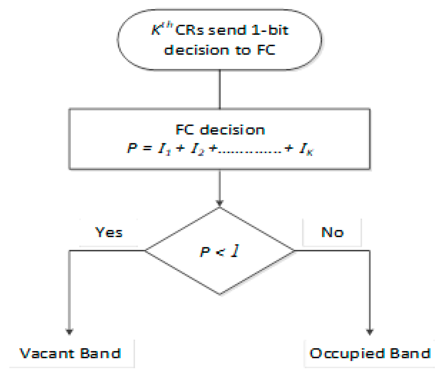
The CSS method holds its usefulness to improve the detection performance of CR users since it minimizes fading and shadowing effects [16]. In CSS, a centralized-CSS is considered where CR users work in more than one or all together as shown in Figure 3. Furthermore, CR local binary decision (0 or 1) is sent to a common FC that takes the final decision. On the other hand, in the de-centralized CSS method, the individual decision is taken by each CR user and then it is passed to each other. This makes de-centralized CSS quite complex and not reliable. Furthermore, in a centralized CSS scheme, it is seen in Figure 3 that k is the number of CRs and their local decision is I_i and these were collected by an FC using the OR-rule decision. FC performs a hard decision method on this collected data to decide the presence of PU signal [17].

Hard decision-based spectrum sensing has been considered. Therefore,

$$P={\displaystyle \sum _{i=1}^k{I}_i}$$

(47)

P is the summation of the local binary decisions I_i sent by ith CRs. I_i is the output of the proposed sensing scheme and it can be defined in the form of pre-defined thresholds as shown in Equation (48).

$$I_i=\{\begin{array}{c}\begin{array}{cccc}1,& {\lambda }_1\le E& or& \gamma \le Z\end{array}\\ \begin{array}{cccc}0,& E<{\lambda }_1& or& Z<\gamma \end{array}\end{array}$$

(48)

For global conclusion, the final output of FC expressed in functional representation form using the hard decision OR-rule can be shown as:

$$FC=\{\begin{array}{c}\begin{array}{cc}P<1,& H_0\end{array}\\ \begin{array}{cc}P\ge 1,& H_1\end{array}\end{array}$$

(49)

The examination of the CSS performance with the proposed scheme can be done via detection probability (P_D). Therefore, the P_D of the FC is expressed as

$$P_D=P_r\left\{{\displaystyle \sum _{j=1}^k{I}_i}\ge 1|H_1\right\}$$

(50)

$$P_D=1-{\displaystyle \prod _{j=1}^k\left(1-P_{d,j}\right)}$$

(51)

In Equation (51), the detection probability of individual CR user is represented by Pd which is computed using Equation (4).

Simulation Model

By using MATLAB, the simulation environment is created and the simulation steps are given below:

• Repeat the above steps numbered from 1 to 9. This will generate local decisions using CRs according to Equation (48) from where they are sent to FC.
• CR’s output is collected by FC according to Equation (47).
• Finally, hard decision OR-rule at FC using Equation (49) is considered to claim hypothesis H₀ or H₁.
• Steps 1 to 3 are repeated up to 1000 times to evaluate the Pd versus SNR under consideration that P_f is fixed at 0.1.

5. Simulation Results and Analysis

Figure 4 depicts the network distribution using NetSim software.

Table 1. Deployed parameters.

Parameter	Value
Signal type	QPSK
False alarm probability	0.1
Sample number (N)	1000
Threshold (λ)	−6 dB
Threshold (λ1)	1.2 dB
Threshold ($\gamma$)	1.15
Threshold (${\gamma }_1$)	0.9
Threshold (${\gamma }_2$)	1.4
Probability factor (Pr)	0.5
Software	NetSim and MATLAB

shows the simulation parameters to be assumed to get the results. Furthermore, the proposed technique is compared with, ED and Cyclo-2010 [1], ASS-2012 [3], ED and ED-ADT-2013 [6], EDT-ASS-2015 [7], and ESNR-ADT detector-2016 [9].

IEEE 802.22 states that the minimum detection probability is 0.9 for the false alarm probability (P_f) of 0.1. It means the implemented technique will detect PU signals below −12.0 dB SNR as seen in Figure 5. The detection probability of the proposed scheme beats ED and ED-ADT-2013 by 33.5%, ASS-2012 by 41.5%, ED and Cyclo-2010 by 57.0%, ESNR-ADT detector-2016 by 52.8%, and EDT-ASS-2015 by 28.2% at −12 dB SNR, respectively.

In

Table 2. Comparison among detectors regarding the probability of detection.

Sensing Detector	Detection Performance (%)
ED and ED-ADT-2013	68.31
ED and Cyclo-2010	61.43
ASS-2012	67.99
EDT-ASS-2015	67.90
ESNR-ADT detector-2016	66.25
Proposed scheme	79.25

, the proposed sensor-based smart detection technique shows a 79.27% detection performance. Consequently, it senses or forecasts accurate information of PU signal presence or noise better than any other sensing strategies.

The performance of the proposed scheme in terms of P_e is shown in Figure 6. The suggested method has a smaller error rate than the current sensing approaches and the proposed system achieves P_e = 0.1 at −8 dB SNR.

Table 3. Comparison of detectors according to their error rates.

Sensing Detector	Error Rate (%)
ED and ED-ADT-2013	10.00
ED and Cyclo-2010	23.00
ASS-2012	25.10
EDT-ASS-2015	15.40
ESNR-ADT detector-2016	11.00
Proposed scheme	<10.00

shows that the proposed scheme has a smaller error rate of below 10%. It shows our detector has more accuracy than others.

Receiver operating characteristic (ROC) graphs in Figure 7 show the relationship between P_d and P_f. The behavior of P_d and P_f for various SNR values such as (−6 dB, −8 dB, −10 dB, −12 dB, and −14 dB) is plotted in Figure 7. The values of P_d and P_f are always above 0.9 and 0.1, respectively for all the values of SNR who are greater than −12 dB. The proposed detector can detect those PU signals whose SNR value is above or at least −12 dB.

IEEE 802.22 recommends that the detection time by CRs for the user’s spectrum bands must be as small as possible. Figure 8 shows that the proposed technique performs well and takes lesser time than existing sensing techniques except for EDT-ASS-2015.

IEEE 802.22 states that sensing time for any detector to detect the PU signal should be as small as possible. In Figure 8, the proposed scheme requires 45.52 ms sensing time at −20 dB whereas 44.48 ms at 0 dB SNR, which is lesser than ED and Cyclo-2010, ED and ED-ADT-2013, ESNR-ADT detector-2016, and ASS-2012.

In

Table 4. Comparison of detectors concerning their sensing times.

Sensing Detector	Sensing Time (Millisecond)
ED and ED-ADT-2013	43.7909
ED and Cyclo-2010	48.4636
ASS-2012	46.2564
EDT-ASS-2015	45.2564
ESNR-ADT detector-2016	45.5521
Proposed scheme	45.5218

, the proposed smart sensor-based detection scheme takes 45.5218 ms to detect the correct signal. It shows that the proposed detector requires less observation time, except for EDT-ASS-2015.

Figure 9 shows the graphs between P_d and threshold values for various SNR values such as −6 dB, −8 dB, −10 dB, −12 dB, and −14 dB. It can be seen that P_d provides different results at different threshold values for different SNRs. IEEE 802.22 defines that if P_f is 0.1, then the minimum P_d value must be 0.9. This minimum value of P_d declares whether the PU signal is present or not. Therefore, it can be concluded that the proposed detector produces the best results at −6 dB SNR throughout the range of threshold values.

Table 5. Comparisons of cooperative detectors.

Sensing Detector	Detector Performance (%)
HwQ-2012	73.92
CSS-EDT-ASS-2015	78.07
Proposed scheme	84.33

displays the comparisons of cooperative detectors. It can be seen that the proposed scheme produces the best detection performance when all CRs work collaboratively.

Figure 10 shows the P_d versus SNR graphs between the proposed scheme with CSS, hierarchical with quantization-2012 (HwQ-2012), and cooperative-EDT-ASS-2015 detection techniques. In CSS, three CR users are assumed to be included.

Results indicate that CSS with the proposed scheme outperforms CSS-EDT-ASS-2015 and HwQ-2012 by 16.10% and 22.70% at −12 dB SNR, respectively. CSS with the proposed scheme attains 0.9 detection probability at −12.50 dB while EDT-ASS-2015 and HwQ-2012 methods achieve the same rate at −10.75 dB and −10.25 dB, respectively.

Figure 11 shows that detection probability improves as the amount of CRs rise. In the simulation, P_f was set at 0.1, and the number of CRs (k) is taken as 3, 4, 5, 6, 7, 8, 9, and 10. It was seen that the optimal value of P_d exists at k = 10 which means that 10 CR users together can detect PU signal till −19.70 dB SNR values.

6. Conclusions

In this study, a new smart sensor-based detection scheme for communication has been introduced. The detection efficiency can be increased by using the new sensing system, and it also overcomes problems of sensing loss. Simulation tests show that the new system is leading the current approaches in the area of detection probability. In addition to the enhancement of detection performance, it is concluded that the introduced scheme also performs well within detection time. Furthermore, the detector detects the PU signal at −19.70 dB SNR with a combination of the proposed model and CSS.

Basically, in the proposed model, it was focused on the data transmission/communication between sensors/nodes, and for this, a sensing technique was proposed that senses the signal and share between the nodes. During the data sense, there is a sensing failure problem that may be occurred which can degrade the system performance. In our proposed model, we tried to reduce the sensing failure problem.

The proposed detection technique is useful for every kind of wireless communication link. The novelty of this scheme is that the confused region is divided into two levels (01 and 10) as shown in Figure 1, whereas, earlier there were four levels (00, 01, 10, and 11) as discussed in the literature. Simulation results confirm that using a two-parts confused region scheme, our proposed detector model can enhance detection performance and it takes admissible sensing time to decide whether the PU frequency band is busy or free.

That is why the proposed two-part confused region scheme makes our sensing scheme differ and novel from the existing schemes. However, to the best of available sources, none of the researchers have discussed this detection technique with the assumptions earlier. The proposed scheme is an advanced version of ESNR-ADT detector-2016 and gives better results as discussed in the result and analysis section.

As future work, an appropriate sensor will be constructed with the proposed detection scheme. Real-life experiments will be carried out to compare the experimental results with the simulated results. Simulated results can be improved with the development of new algorithms.