Efficient Implementations for Orthogonal Matching Pursuit

Abstract

Based on the efficient inverse Cholesky factorization, we propose an implementation of OMP (called as version 0, i.e., v0) and its four memory-saving versions (i.e., the proposed v1, v2, v3 and v4). In the simulations, the proposed five versions and the existing OMP implementations have nearly the same numerical errors. Among all the OMP implementations, the proposed v0 needs the least computational complexity, and is the fastest in the simulations for almost all problem sizes. As a tradeoff between computational complexities/time and memory requirements, the proposed v1 seems to be better than all the existing ones when only considering the efficient OMP implementations storing $\mathbf{G}$ (i.e., the Gram matrix of the dictionary), the proposed v2 and v3 seem to be better than the only existing one when only considering the efficient implementations not storing $\mathbf{G}$, and the proposed v4 seems to be better than the naive implementation that has the (known) minimum memory requirements. Moreover, all the proposed five versions only include parallelizable matrix-vector products in each iteration, and do not need any back-substitutions that are necessary in some existing efficient implementations (e.g., those utilizing the Cholesky factorization).

1. Introduction

A signal vector $\mathbf{x}\in {\mathbb{C}}^N$ is said to be K-sparse if $\mathbf{x}$ includes no more than K none-zero entries. The measurements of the signal $\mathbf{x}$ can be collected in a data vector $\mathbf{u}\in {\mathbb{C}}^M$ satisfying

$$\mathbf{u}=\mathbf{\Phi }\mathbf{x}+\mathbf{n},$$

(1)

where $\mathbf{\Phi }$ is an $M\times N$ dictionary with $K<M\ll N$, and $\mathbf{n}$ is noise. The problem of signal recovery, i.e., solving (1) to estimate $\mathbf{x}$, is sparse approximation or representation [1,2,3,4,5,6].

Recently, the OMP algorithm has been applied in various scenarios [7,8,9,10,11,12,13]. The stagewise OMP algorithm was proposed in [7] to enhance the convergence speed for switching signal reconstruction in IGBT (insulated gate bipolar transistor) online condition monitoring, while the SiT based stagewise OMP was propopsed in [8] for the estimation of massive-MIMO sparse uplink channels. A modified OMP algorithm was utilized in [9] to propose compressed sensing ISAR (inverse synthetic aperture radar) imaging with highly maneuvering motion. The OMP algorithm was used in [10] for AoD (angle of departure) estimation at the mobile station, applied in [11] for channel estimation and equalization on the basis of the Pseudo-Noise (PN) sequences, and was chosen in [12] as the imaging algorithm to reconstruct imaging scenes in the single-pixel camera, since it contains the stable and efficient operation in reconstructing small data. Moreover, simultaneous OMP [14] was utilized in [13] to convert image patches into sparse coefficients for representing the source multi-focus images.

The computational complexity of OMP can be reduced by utilizing the Cholesky factorization [15,16,17], the QR factorization [18,19,20], or the Matrix Inversion Lemma (MIL) [20,21,22,23] that is also called as Matrix Inversion Bypass (MIB). Most of the efficient implementations of OMP in [15,16,17,18,19,20,21,22,23] have been compared in [24]. Hardware-efficient architectures of OMP based on Cholesky factorization, QR factorization and MIL have been reported in [25,26,27,28,29,30,31,32,33,34], respectively. Moreover, to implement simultaneous OMP [14] efficiently, a novel partitioned inversion method was proposed in [35].

Based on the efficient inverse Cholesky factorization proposed in [36], we propose an efficient OMP implementation and its four memory-saving versions (This work was presented partly in [37] at IEEE Vehicular Technology Conference (VTC) 2013 fall. The new contribution in this manuscript includes the memory-saving versions 1 and 4, the derivation of the equations in the proposed OMP implementations, the more detailed introduction of the existing OMP implementations, and the more detailed comparison among the presented OMP implementations), which are then compared with the existing ones. To focus on efficient implementations of OMP, we do not consider the extended, variant, or approximate implementations of OMP, such as the Stagewise OMP (StOMP) [38], the Backtracking-based Adaptive OMP (BAOMP) [39], the gradient pursuit [40], or the cyclic matching pursuit [41].

This paper is organized as follows. Section 2 describes the existing implementations for OMP. In Section 3, we propose an efficient OMP implementation and its four memory-saving versions. Then in Section 4, we evaluate the presented implementations for OMP. Finally, we make conclusion in Section 5.

In what follows, ${(•)}^T$, ${(•)}^{*}$, and ${(•)}^H$ denote the matrix transposition, the matrix conjugate, and the Hermitian matrix, respectively. We use ${\mathbf{0}}_M$, ${\mathrm{I}}_M$ and ∅ to denote the length-M zero column vector, the $M\times M$ identity matrix and the empty matrix (or vector), respectively, and we use $\parallel ·\parallel$ to denote the square norm (i.e., the $L^2$ norm) of a vector.

2. The Existing Implementations for OMP

In this section, we summarize the existing OMP implementations.

2.1. The Naive Implementation of OMP

The dictionary $\mathbf{\Phi }$ in (1) can be written as

$$\mathbf{\Phi }=\left(\begin{array}{cccc}{\phi }_{:1}& {\phi }_{:2}& \cdots & {\phi }_{:N}\end{array}\right),$$

(2)

where ${\phi }_{:i}\in C^M$ denotes the i-th column of $\mathbf{\Phi }$, and is called as an atom. The signal recovery problem is to find the sparse solution to the underdetermined linear system (1), i.e., to represent $\mathbf{u}$ as a weighted sum of the least number of atoms. OMP is a greedy algorithm that selects atoms from $\mathbf{\Phi }$ iteratively to approximate $\mathbf{u}$ gradually. In each iteration, OMP selects the atom best matching the current residual (i.e., the approximation error), renews the weights for all the already selected atoms to obtain the least squares approximation of $\mathbf{u}$, and then updates the residual accordingly.

Algorithm 1 summarizes the naive implementation of OMP [20,24], which is called Naive in this paper, as in [24]. As the OMP implementation described in ([20] (left lines 27–34 on page 2)), we also follow these conventions: ${\mathbf{\Lambda }}_k$ is a set containing the indices of the selected k atoms, and ${\mathbf{\Phi }}_{{\mathbf{\Lambda }}_k}$ is a sub-matrix of $\mathbf{\Phi }$ containing only those columns of $\mathbf{\Phi }$ with indices in ${\mathbf{\Lambda }}_k$. The estimate $\widehat{\mathbf{x}}$ for $\mathbf{x}$ has nonzero entries at the indices listed in ${\mathbf{\Lambda }}_k$, and the ${\lambda }_i$-th entry of $\widehat{\mathbf{x}}$ equals the i-th entry of ${\widehat{\mathbf{x}}}_k$.

Algorithm 1 The Naive Implementation of OMP

Step 1. : Initialize ${\mathbf{\Lambda }}_0=\varnothing$, the residual ${\mathbf{r}}^0=\mathbf{u}$, and the iteration counter $k=1$. Step 2. : Projection: compute the inner products $${\mathbf{p}}^{k-1}={\mathbf{\Phi }}^H{\mathbf{r}}^{k-1}.$$ (3) Step 3. : Decide $i^k={\mathrm{argmax}}_{i=1,2,\cdots ,N}\left(\left|p_i^{k-1}\right|/∥{\phi }_{:i}∥\right)$, where $p_i^{k-1}$ is the i-th entry of ${\mathbf{p}}^{k-1}$. Let ${\mathbf{\Lambda }}_k={\mathbf{\Lambda }}_{k-1}\cup \left\{i^k\right\}$, i.e., ${\lambda }_k\triangleq i^k$ is the k-th entry of the set ${\mathbf{\Lambda }}_k$. Step 4. : Renew the weights for the selected k atoms by $${\widehat{\mathbf{x}}}_k={\left({\mathbf{\Phi }}_{{\mathbf{\Lambda }}_k}^H{\mathbf{\Phi }}_{{\mathbf{\Lambda }}_k}\right)}^{-1}{\mathbf{\Phi }}_{{\mathbf{\Lambda }}_k}^H\mathbf{u},$$ (4) and then utilize ${\widehat{\mathbf{x}}}_k$ to update the residual by $${\mathbf{r}}^k=\mathbf{u}-{\mathbf{\Phi }}_{{\mathbf{\Lambda }}_k}{\widehat{\mathbf{x}}}_k.$$ (5) Step 5. : $k:=k+1$. Then return to Step 2 if $k<K$ and the residual energy [24] $${∥{\mathbf{r}}^k∥}^2>\xi {∥\mathbf{u}∥}^2,$$ (6) where $\xi$ is a small positive real number, e.g., $\xi ={10}^{-10}$. Step 6. : Output: ${\mathbf{r}}^{K^{\prime }}$, ${\mathbf{\Lambda }}_{K^{\prime }}$ and ${\widehat{\mathbf{x}}}_{K^{\prime }}$, where $K^{\prime }\le K$.

2.2. The Existing Efficient Implementations of OMP

To implement OMP efficiently, the Cholesky factorization has been applied in [15,16,17,25,26,27,28], the QR factorization has been applied in [18,19,20,29,30,31], and the MIL (i.e., Matrix Inversion Lemma) has been applied in [20,21,22,23,32,33,34]. In [24], the authors summarized the existing various implementations of OMP in [15,16,17,18,19,20,21,22,23], studied their numerical and computational performances, and empirically compared their computational time. According to the conclusions in [24], the accumulation of error is insignificant in each existing OMP implementation. On the other hand, any of the existing implementations compared in [24] can be the fastest for some specific problem sizes, while the efficient OMP implementation by the QR factorization [19] appears to be the fastest for particularly large problem sizes.

In the rest of this subsection, we introduce the existing efficient implementations of OMP, including two implementations by the Cholesky factorization [15,16,17] and two implementations by the QR factorization [19], which are called as Chol-1, Chol-2, QR-1 and QR-2, respectively, as in [24]. Moreover, we also include two implementations by the MIL (i.e., Matrix Inversion Lemma) discussed in [21,24], i.e., MIL-1 and MIL-2. Since the literatures [25,26,27,28,29,30,31,32,33,34] mainly deal with the hardware architectures for the existing OMP implementations, we will not introduce the OMP implementations in [25,26,27,28,29,30,31,32,33,34] in the rest of this subsection.

For simplicity, we assume that the dictionary $\mathbf{\Phi }$ has normalized columns, i.e., ${∥{\phi }_{:i}∥}^2=1$, as in [18] and the shared simulation code [42] of [24]. We omit step 6 to only focus on the k-th iteration, and we omit steps 1, 3 and 5, since they are the same as those in Algorithm 1 except that now it is required to initialize ${∥{\mathbf{r}}^0∥}^2={∥\mathbf{u}∥}^2$ in step 1. Thus we only introduce steps 2 and 4, which update the projection ${\mathbf{p}}^{k-1}$ and the residual energy ${∥{\mathbf{r}}^k∥}^2$, respectively.

Many existing efficient OMP implementations utilize the Gram matrix [20] of all the N atoms ${\phi }_{:1}$, ${\phi }_{:2}$, ⋯, ${\phi }_{:N}$, i.e.,

$$\mathbf{G}={\mathbf{\Phi }}^H\mathbf{\Phi }.$$

(7)

The Gram matrix of the k atoms selected in iteration k is

$${\mathbf{G}}_{{\mathbf{\Lambda }}_k}={\mathbf{\Phi }}_{{\mathbf{\Lambda }}_k}^H{\mathbf{\Phi }}_{{\mathbf{\Lambda }}_k},$$

(8)

where ${\mathbf{\Phi }}_{{\mathbf{\Lambda }}_k}$ can be written as

$${\mathbf{\Phi }}_{{\mathbf{\Lambda }}_k}=\left[\begin{array}{cc}{\mathbf{\Phi }}_{{\mathbf{\Lambda }}_{k-1}}& {\phi }_{:{\lambda }_k}\end{array}\right].$$

(9)

In Algorithm 2 we introduce Chol-1 and Chol-2, which utilize the Cholesky factor [43] of ${\mathbf{G}}_{{\mathbf{\Lambda }}_k}$, i.e., ${\mathbf{V}}_k$ satisfying

$${\mathbf{V}}_k{\mathbf{V}}_k^H={\mathbf{G}}_{{\mathbf{\Lambda }}_k}.$$

(10)

We also need

$${\mathbf{s}}_{k-1}={\mathbf{\Phi }}_{{\mathbf{\Lambda }}_{k-1}}^H{\phi }_{:{\lambda }_k},$$

(11)

which is obtained in ${\mathbf{G}}_{{\mathbf{\Lambda }}_k}$ by

$${\mathbf{G}}_{{\mathbf{\Lambda }}_k}=\left[\begin{array}{cc}{\mathbf{G}}_{{\mathbf{\Lambda }}_{k-1}}& {\mathbf{s}}_{k-1}\\ {\mathbf{s}}_{k-1}^H& g_{{\lambda }_k,{\lambda }_k}\end{array}\right].$$

(12)

To verify (12) and (11), substitute (9) into (8) to deduce

$${\mathbf{G}}_{{\mathbf{\Lambda }}_k}=\left[\begin{array}{cc}{\mathbf{\Phi }}_{{\mathbf{\Lambda }}_{k-1}}^H{\mathbf{\Phi }}_{{\mathbf{\Lambda }}_{k-1}}& {\mathbf{\Phi }}_{{\mathbf{\Lambda }}_{k-1}}^H{\phi }_{:{\lambda }_k}\\ {\phi }_{:{\lambda }_k}^H{\mathbf{\Phi }}_{{\mathbf{\Lambda }}_{k-1}}& {\phi }_{:{\lambda }_k}^H{\phi }_{:{\lambda }_k}\end{array}\right].$$

(13)

In Algorithm 3 we introduce QR-1 and QR-2, which utilize the QR factors [19] of ${\mathbf{\Phi }}_{{\mathbf{\Lambda }}_k}$, i.e., ${\mathbf{Q}}_k$ and ${\mathbf{R}}_k$ satisfying

$${\mathbf{\Phi }}_{{\mathbf{\Lambda }}_k}={\mathbf{Q}}_k{\mathbf{R}}_k.$$

(14)

In Algorithm 4 we introduce MIL-1 and MIL-2. In each iteration, MIL-1 updates the biorthogonal basis of ${\mathbf{\Phi }}_{{\mathbf{\Lambda }}_k}$, i.e.,

$${\mathbf{\Psi }}_{{\mathbf{\Lambda }}_k}={\mathbf{\Phi }}_{{\mathbf{\Lambda }}_k}{\left({\mathbf{\Phi }}_{{\mathbf{\Lambda }}_k}^H{\mathbf{\Phi }}_{{\mathbf{\Lambda }}_k}\right)}^{-1}$$

(15)

satisfying

$${\mathbf{\Psi }}_{{\mathbf{\Lambda }}_k}^H{\mathbf{\Phi }}_{{\mathbf{\Lambda }}_k}={\mathbf{\Phi }}_{{\mathbf{\Lambda }}_k}^H{\mathbf{\Psi }}_{{\mathbf{\Lambda }}_k}=\mathbf{I},$$

(16)

while MIL-2 updates ${\mathbf{G}}_{{\mathbf{\Lambda }}_k}^{-1}$.

Algorithm 2 OMP by the Cholesky Decomposition

Step 2. Projection: if $k=1$, compute ${\mathbf{p}}^0$ by (3); else when $k\ge 2$, compute ${\widehat{\mathbf{x}}}_{k-1}$ by solving the triangular system $${\mathbf{V}}_{k-1}^H{\widehat{\mathbf{x}}}_{k-1}={\mathbf{y}}_{k-1},$$ (17) and then compute ${\mathbf{p}}^{k-1}$ by one of two ways. In the first case (Chol-1), explicitly compute ${\mathbf{r}}^{k-1}$ ($k\ge 2$) by (5) and then directly compute ${\mathbf{p}}^{k-1}$ ($k\ge 2$) by (3); or in the second case (Chol-2), compute ${\mathbf{p}}^{k-1}$ ($k\ge 2$) by $${\mathbf{p}}^{k-1}={\mathbf{p}}^0-\mathbf{G}(:,{\mathbf{\Lambda }}_{k-1})·{\widehat{\mathbf{x}}}_{k-1},$$ (18) where $\mathbf{G}(:,{\mathbf{\Lambda }}_{k-1})$ includes $k-1$ columns in $\mathbf{G}$ and satisfies $$\mathbf{G}(:,{\mathbf{\Lambda }}_{k-1})={\mathbf{\Phi }}^H{\mathbf{\Phi }}_{{\mathbf{\Lambda }}_{k-1}}.$$ (19) Step 4. If $k=1$, obtain ${\mathbf{V}}_1=1$ from (10); else when $k\ge 2$, obtain ${\mathbf{V}}_k$ by $${\mathbf{V}}_k=\left[\begin{array}{cc}{\mathbf{V}}_{k-1}& {\mathbf{0}}_{k-1}\\ {\mathbf{z}}_{k-1}^H& \sqrt{g_{{\lambda }_k,{\lambda }_k}-{∥{\mathbf{z}}_{k-1}∥}^2}\end{array}\right],$$ (20) where $g_{{\lambda }_k,{\lambda }_k}={\phi }_{:{\lambda }_k}^H{\phi }_{:{\lambda }_k}$ is in $\mathbf{G}$, and ${\mathbf{z}}_{k-1}$ is computed by solving the triangular system $${\mathbf{V}}_{k-1}{\mathbf{z}}_{k-1}={\mathbf{s}}_{k-1}={\mathbf{\Phi }}_{{\mathbf{\Lambda }}_{k-1}}^H{\phi }_{:{\lambda }_k}.$$ (21) Then for any $k\ge 1$, compute ${\mathbf{y}}_k$ by solving $${\mathbf{V}}_k{\mathbf{y}}_k={\mathbf{p}}_{{\mathbf{\Lambda }}_k}^0={\mathbf{\Phi }}_{{\mathbf{\Lambda }}_k}^H\mathbf{u},$$ (22) where $${\mathbf{p}}_{{\mathbf{\Lambda }}_k}^0={\left[\begin{array}{cccc}{p}_{{\lambda }_1}^0& p_{{\lambda }_2}^0& \cdots & p_{{\lambda }_k}^0\end{array}\right]}^T$$ (23) has the i-th entry $p_{{\lambda }_i}^0$ ($1\le i\le k$) being the ${\lambda }_i$-th entry in ${\mathbf{p}}^0$, and finally compute ${∥{\mathbf{r}}^k∥}^2={∥\mathbf{u}∥}^2-{∥{\mathbf{y}}_k∥}^2$.

Algorithm 3 OMP by the QR Decomposition

Step 2. Projection: if $k=1$, compute ${\mathbf{p}}^0$ by (3); else compute ${\mathbf{p}}^{k-1}$ ($k\ge 2$) by one of two ways. In the first case (QR-1), compute ${\mathbf{p}}^{k-1}$ ($k\ge 2$) by $${\mathbf{p}}^{k-1}={\mathbf{p}}^{k-2}-\left({\mathbf{q}}_{:k-1}^H\mathbf{u}\right){\mathbf{\Phi }}^H{\mathbf{q}}_{:k-1}$$ (24) where ${\mathbf{q}}_{:k-1}$ denotes the $(k-1)$-th column in ${\mathbf{Q}}_{k-1}$; or in the second case (QR-2), compute ${\mathbf{y}}_{k-1}$ ($k\ge 2$) by solving the triangular system $${\mathbf{R}}_{k-1}^H{\mathbf{y}}_{k-1}={\mathbf{p}}_{{\mathbf{\Lambda }}_{k-1}}^0={\mathbf{\Phi }}_{{\mathbf{\Lambda }}_{k-1}}^H\mathbf{u},$$ (25) compute ${\widehat{\mathbf{x}}}_{k-1}$ ($k\ge 2$) by solving $${\mathbf{R}}_{k-1}{\widehat{\mathbf{x}}}_{k-1}={\mathbf{y}}_{k-1},$$ (26) and then compute ${\mathbf{p}}^{k-1}$ ($k\ge 2$) by (18). Step 4. If $k=1$, obtain ${\mathbf{Q}}_1$ and ${\mathbf{R}}_1$ from (14); else when $k\ge 2$, compute $${\mathbf{w}}_{k-1}={\mathbf{Q}}_{k-1}^H{\phi }_{:{\lambda }_k}$$ (27) and $${\beta }_k=\sqrt{g_{{\lambda }_k,{\lambda }_k}-{∥{\mathbf{w}}_{k-1}∥}^2},$$ (28) to obtain $${\mathbf{Q}}_k=\left[\begin{array}{cc}{\mathbf{Q}}_{k-1}& ({\phi }_{:{\lambda }_k}-{\mathbf{Q}}_{k-1}{\mathbf{w}}_{k-1})/{\beta }_k\end{array}\right]$$ (29) and $${\mathbf{R}}_k=\left[\begin{array}{cc}{\mathbf{R}}_{k-1}& {\mathbf{w}}_{k-1}\\ {\mathbf{0}}_{k-1}^T& {\beta }_k\end{array}\right],$$ (30) and finally compute ${∥{\mathbf{r}}^k∥}^2={∥{\mathbf{r}}^{k-1}∥}^2-{\left|{\mathbf{q}}_{:k}^H\mathbf{u}\right|}^2$.

Algorithm 4 OMP by the Matrix Inversion Lemma

Step 2. Projection: if $k=1$, compute ${\mathbf{p}}^0$ by (3); else compute $${\mathbf{p}}^{k-1}={\mathbf{p}}^{k-2}+{\delta }_{k-1}\mathbf{G}(:,{\mathbf{\Lambda }}_{k-1}){\left[\begin{array}{cc}{\mathbf{h}}_{k-2}^T& -1\end{array}\right]}^T,$$ (31) where $k\ge 2$, and ${\mathbf{h}}_0=\varnothing$ when $k=2$. Step 4. If $k=1$, compute ${\epsilon }_1=1/g_{{\lambda }_1,{\lambda }_1}$ and ${\delta }_1={\epsilon }_1{p}_{{\lambda }_1}^0$, and obtain ${\mathbf{\Psi }}_{{\mathbf{\Lambda }}_1}$ by (15) for MIL-1 or ${\mathbf{G}}_{{\mathbf{\Lambda }}_1}^{-1}=1/{\mathbf{G}}_{{\mathbf{\Lambda }}_1}$ for MIL-2; else compute the intermediate results by one of two ways. In the first case (MIL-1) when $k\ge 2$, compute $${\psi }_{:k-1}={\epsilon }_{k-1}({\phi }_{:{\lambda }_{k-1}}-{\overline{\mathbf{v}}}^{k-1})$$ (32) to obtain $${\mathbf{\Psi }}_{{\mathbf{\Lambda }}_{k-1}}=\left[\begin{array}{cc}\left({\mathbf{\Psi }}_{{\mathbf{\Lambda }}_{k-2}}-{\psi }_{:k-1}{\mathbf{h}}_{k-2}^H\right)& {\psi }_{:k-1}\end{array}\right],$$ (33) compute $${\mathbf{h}}_{k-1}={\mathbf{\Psi }}_{{\mathbf{\Lambda }}_{k-1}}^H{\phi }_{:{\lambda }_k},$$ (34) $${\overline{\mathbf{v}}}^k={\mathbf{\Phi }}_{{\mathbf{\Lambda }}_{k-1}}{\mathbf{h}}_{k-1},$$ (35) $${\epsilon }_k=1/\left(g_{{\lambda }_k,{\lambda }_k}-{∥{\overline{\mathbf{v}}}^k∥}^2\right)$$ (36) and $${\delta }_k={\epsilon }_k\left(p_{{\lambda }_k}^0-{\mathbf{h}}_{k-1}^H{\mathbf{p}}_{{\mathbf{\Lambda }}_{k-1}}^0\right);$$ (37) or in the second case (MIL-2) when $k\ge 2$, compute $${\mathbf{G}}_{{\mathbf{\Lambda }}_{k-1}}^{-1}=\left[\begin{array}{cc}{\mathbf{G}}_{{\mathbf{\Lambda }}_{k-2}}^{-1}+{\epsilon }_{k-1}{\mathbf{h}}_{k-2}{\mathbf{h}}_{k-2}^H& -{\epsilon }_{k-1}{\mathbf{h}}_{k-2}\\ -{\epsilon }_{k-1}{\mathbf{h}}_{k-2}^H& {\epsilon }_{k-1}\end{array}\right],$$ (38) obtain ${\mathbf{s}}_{k-1}$ in ${\mathbf{G}}_{{\mathbf{\Lambda }}_k}$ by (12) to compute $${\mathbf{h}}_{k-1}={\mathbf{G}}_{{\mathbf{\Lambda }}_{k-1}}^{-1}{\mathbf{s}}_{k-1}$$ (39) and $${\epsilon }_k=1/\left(g_{{\lambda }_k,{\lambda }_k}-{\mathbf{s}}_{k-1}^H{\mathbf{h}}_{k-1}\right),$$ (40) and compute ${\delta }_k$ by (37). Finally compute $${∥{\mathbf{r}}^k∥}^2={∥{\mathbf{r}}^{k-1}∥}^2+{\left|{\delta }_k\right|}^2/{\epsilon }_k-2\mathrm{Re}\left\{{\delta }_k{p}_{{\lambda }_k}^{k-1}\right\}.$$ (41)

3. The Proposed Efficient OMP Implementation and Its Memory-Saving Versions

In this section, we propose an efficient OMP implementation, which is based on the efficient inverse Cholesky factorization proposed in [36]. We also introduce four memory-saving versions for the proposed OMP implementation.

3.1. The Proposed OMP Implementation by the Inverse Cholesky Factorization

The inverse Cholesky factor [36] of ${\mathbf{G}}_{{\mathbf{\Lambda }}_k}$ can be denoted as ${\mathbf{F}}_k$ satisfying

$${\mathbf{F}}_k{\mathbf{F}}_k^H={\mathbf{G}}_{{\mathbf{\Lambda }}_k}^{-1}={\left({\mathbf{\Phi }}_{{\mathbf{\Lambda }}_k}^H{\mathbf{\Phi }}_{{\mathbf{\Lambda }}_k}\right)}^{-1},$$

(42)

while from (10) we can deduce

$${\mathbf{V}}_k^{-H}{\mathbf{V}}_k^{-1}={\mathbf{G}}_{{\mathbf{\Lambda }}_k}^{-1}.$$

(43)

Then we can compare (43) with (42) to deduce

$${\mathbf{F}}_k={\mathbf{V}}_k^{-H},$$

(44)

since ${\mathbf{V}}_k$ is the unique lower-triangular Cholesky factor [43] of ${\mathbf{G}}_{{\mathbf{\Lambda }}_k}$, and ${\mathbf{F}}_k$, the upper-triangular equivalent Cholesky factor of ${\mathbf{G}}_{{\mathbf{\Lambda }}_k}^{-1}$ [36], is also unique [43].

In [36], ${\mathbf{F}}_k$ is computed from ${\mathbf{F}}_{k-1}$ iteratively by

$${\mathbf{F}}_k=\left[\begin{array}{cc}{\mathbf{F}}_{k-1}& {\mathbf{t}}_{k-1}\\ {\mathbf{0}}_{k-1}^T& {\gamma }_k\end{array}\right],$$

(45)

where ${\gamma }_k$ and ${\mathbf{t}}_{k-1}$ is computed by ([36] (Equation (24)))

$${\gamma }_k=1/\sqrt{g_{{\lambda }_k,{\lambda }_k}-{\mathbf{c}}_{k-1}^H{\mathbf{c}}_{k-1}},$$

(46)

$${\mathbf{t}}_{k-1}=-{\gamma }_k{\mathbf{F}}_{k-1}{\mathbf{c}}_{k-1},$$

(47)

and

$${\mathbf{c}}_{k-1}={\mathbf{F}}_{k-1}^H{\mathbf{s}}_{k-1}.$$

(48)

Notice that ${\mathbf{s}}_{k-1}$ in (48) and $g_{{\lambda }_k,{\lambda }_k}$ in (46) are the vector and scalar in ${\mathbf{G}}_{{\mathbf{\Lambda }}_k}$, respectively, as shown in (12).

To utilize ${\mathbf{F}}_k$ in OMP, we substitute (42) into (4) to deduce

$${\widehat{\mathbf{x}}}_k={\mathbf{F}}_k{\mathbf{F}}_k^H{\mathbf{\Phi }}_{{\mathbf{\Lambda }}_k}^H\mathbf{u}.$$

(49)

Then we substitute (49) into (5) to obtain ${\mathbf{r}}^k=\mathbf{u}-{\mathbf{\Phi }}_{{\mathbf{\Lambda }}_k}{\mathbf{F}}_k{\mathbf{F}}_k^H{\mathbf{\Phi }}_{{\mathbf{\Lambda }}_k}^H\mathbf{u}$, which is substituted into (3) to obtain

$${\mathbf{p}}^{k-1}={\mathbf{\Phi }}^H\mathbf{u}-{\mathbf{\Phi }}^H{\mathbf{\Phi }}_{{\mathbf{\Lambda }}_{k-1}}{\mathbf{F}}_{k-1}{\mathbf{F}}_{k-1}^H{\mathbf{\Phi }}_{{\mathbf{\Lambda }}_{k-1}}^H\mathbf{u}.$$

(50)

Equation (50) can be written as

$${\mathbf{p}}^{k-1}={\mathbf{\Phi }}^H\mathbf{u}-{\mathbf{B}}_{k-1}{\mathbf{a}}_{k-1},$$

(51)

where

$${\mathbf{a}}_k={\mathbf{F}}_k^H{\mathbf{\Phi }}_{{\mathbf{\Lambda }}_k}^H\mathbf{u}={\mathbf{E}}_k^H\mathbf{u},$$

(52)

$${\mathbf{B}}_k={\mathbf{\Phi }}^H{\mathbf{\Phi }}_{{\mathbf{\Lambda }}_k}{\mathbf{F}}_k={\mathbf{\Phi }}^H{\mathbf{E}}_k,$$

(53)

and

$${\mathbf{E}}_k={\mathbf{\Phi }}_{{\mathbf{\Lambda }}_k}{\mathbf{F}}_k.$$

(54)

Let us deduce

$${\mathbf{F}}_1=\sqrt{{\mathbf{G}}_{{\mathbf{\Lambda }}_1}^{-1}}=\sqrt{g_{{\lambda }_1,{\lambda }_1}}=\sqrt{{\left({\mathbf{\Phi }}_{{\mathbf{\Lambda }}_1}^H{\mathbf{\Phi }}_{{\mathbf{\Lambda }}_1}\right)}^{-1}}$$

(55)

from (42), and substitute (47) into (45) to obtain

$${\mathbf{F}}_k=\left[\begin{array}{cc}{\mathbf{F}}_{k-1}& -{\gamma }_k{\mathbf{F}}_{k-1}{\mathbf{c}}_{k-1}\\ {\mathbf{0}}_{k-1}^T& {\gamma }_k\end{array}\right].$$

(56)

Then we utilize the above-described intermediate results ${\mathbf{a}}_k$ and ${\mathbf{B}}_k$, to propose an efficient OMP implementation (called as version 0, i.e., v0) in the following Algorithm 5, where steps 1, 3 and 5 are omitted as in Algorithms 2–4. In Algorithm 5, we will use (3), (46), (55), (56) and (5) successively.

Algorithm 5 The Proposed OMP Implementation (v0) by the Inverse Cholesky Factorization

Step 2. Projection: if $k=1$, compute ${\mathbf{p}}^0={\mathbf{\Phi }}^H{\mathbf{r}}^0$; else when $k\ge 2$, compute ${\mathbf{p}}^{k-1}$ ($k\ge 2$) by $${\mathbf{p}}^{k-1}={\mathbf{p}}^{k-2}-{\mathbf{b}}_{:(k-1)}·a_{k-1},$$ (57) where ${\mathbf{b}}_{:(k-1)}$ is the $(k-1)$-th column of ${\mathbf{B}}_{k-1}$, and $a_{k-1}$ is the $(k-1)$-th entry of ${\mathbf{a}}_{k-1}$. Step 4. Obtain $${\mathbf{c}}_{k-1}={\left({\mathbf{b}}_{{\lambda }_k,1:k-1}^H\right)}^H,$$ (58) where ${\mathbf{b}}_{{\lambda }_k,1:k-1}^H$ is the ${\lambda }_k$-th row of ${\mathbf{B}}_{k-1}$. Then compute ${\gamma }_k=1/\sqrt{g_{{\lambda }_k,{\lambda }_k}-{\mathbf{c}}_{k-1}^H{\mathbf{c}}_{k-1}}$, $$a_k={\gamma }_k{p}_{{\lambda }_k}^{k-1},$$ (59) $${\mathbf{a}}_k={\left[\begin{array}{cc}{\mathbf{a}}_{k-1}^T& a_k\end{array}\right]}^T,$$ (60) $${\mathbf{b}}_{:k}={\gamma }_k\left({\mathbf{g}}_{:{\lambda }_k}-{\mathbf{B}}_{k-1}{\mathbf{c}}_{k-1}\right),$$ (61) $${\mathbf{B}}_k=\left[\begin{array}{cc}{\mathbf{B}}_{k-1}& {\mathbf{b}}_{:k}\end{array}\right],$$ (62) where $p_{{\lambda }_k}^{k-1}$ is the ${\lambda }_k$-th entry of ${\mathbf{p}}^{k-1}$, ${\mathbf{g}}_{:{\lambda }_k}$ is the ${\lambda }_k$-th column of $\mathbf{G}$, and ${\mathbf{c}}_0={\mathbf{B}}_0={\mathbf{a}}_0=\varnothing$ is assumed for $k=1$. Finally update the residual energy by $${∥{\mathbf{r}}^k∥}^2={∥{\mathbf{r}}^{k-1}∥}^2-{∥a_k∥}^2.$$ (63) If ${\mathbf{F}}_k$ is required to compute ${\widehat{\mathbf{x}}}_k$ and ${\mathbf{r}}^k$, compute ${\mathbf{F}}_k$ by ${\mathbf{F}}_1=\sqrt{g_{{\lambda }_1,{\lambda }_1}}$ when $k=1$, or by ${\mathbf{F}}_k=\left[\begin{array}{cc}{\mathbf{F}}_{k-1}& -{\gamma }_k{\mathbf{F}}_{k-1}{\mathbf{c}}_{k-1}\\ {\mathbf{0}}_{k-1}^T& {\gamma }_k\end{array}\right]$ when $k\ge 2$. Step 6. Output: ${∥{\mathbf{r}}^{K^{\prime }}∥}^2$ and ${\mathbf{\Lambda }}_{K^{\prime }}$. When ${\widehat{\mathbf{x}}}_{K^{\prime }}$ and ${\mathbf{r}}^{K^{\prime }}$ are required, compute $${\widehat{\mathbf{x}}}_{K^{\prime }}={\mathbf{F}}_{K^{\prime }}{\mathbf{a}}_{K^{\prime }}$$ (64) and ${\mathbf{r}}^{K^{\prime }}=\mathbf{u}-{\mathbf{\Phi }}_{{\mathbf{\Lambda }}_{K^{\prime }}}{\widehat{\mathbf{x}}}_{K^{\prime }}$, where $K^{\prime }\le K$.

In the next subsection, we will verify Equations (57)–(64) in Algorithm 5. Moreover, we will also verify

$${\mathbf{e}}_{:k}={\gamma }_k\left({\phi }_{:{\lambda }_k}-{\mathbf{E}}_{k-1}{\mathbf{c}}_{k-1}\right)$$

(65)

and

$${\mathbf{E}}_k=\left[\begin{array}{cc}{\mathbf{E}}_{k-1}& {\mathbf{e}}_{:k}\end{array}\right],$$

(66)

which can be utilized to update the intermediate result ${\mathbf{E}}_k$.

3.2. To Verify Equations (57)–(66)

Here we verify the above-mentioned Equations (57)–(66), in the order of (64), (58), (65), (66), (61), (62), (59), (60), (57) and (63).

To verify (64), we simply substitute (52) into (49). Then we deduce

$${\mathbf{b}}_{i^k,1:k-1}^H={\phi }_{:i^k}^H{\mathbf{\Phi }}_{{\mathbf{\Lambda }}_{k-1}}{\mathbf{F}}_{k-1}={\phi }_{:{\lambda }_k}^H{\mathbf{\Phi }}_{{\mathbf{\Lambda }}_{k-1}}{\mathbf{F}}_{k-1}$$

(67)

from (53), and substitute (11) into (48) to obtain

$${\mathbf{c}}_{k-1}={\mathbf{F}}_{k-1}^H{\mathbf{\Phi }}_{{\mathbf{\Lambda }}_{k-1}}^H{\phi }_{:{\lambda }_k}.$$

(68)

Finally, we compare (67) with (68) to verify (58).

To verify (65) and (66), let us substitute (9) and (45) into (54) to obtain

$${\mathbf{E}}_k=\left[\begin{array}{cc}{\mathbf{\Phi }}_{{\mathbf{\Lambda }}_{k-1}}{\mathbf{F}}_{k-1}& {\mathbf{\Phi }}_{{\mathbf{\Lambda }}_{k-1}}{\mathbf{t}}_{k-1}+{\gamma }_k{\phi }_{:{\lambda }_k}\end{array}\right],$$

(69)

and substitute (47) into (69) to obtain

$${\mathbf{E}}_k=\left[\begin{array}{cc}{\mathbf{\Phi }}_{{\mathbf{\Lambda }}_{k-1}}{\mathbf{F}}_{k-1}& {\gamma }_k({\phi }_{:{\lambda }_k}-{\mathbf{\Phi }}_{{\mathbf{\Lambda }}_{k-1}}{\mathbf{F}}_{k-1}{\mathbf{c}}_{k-1})\end{array}\right].$$

(70)

Finally, let us substitute (54) into (70) to obtain

$${\mathbf{E}}_k=\left[\begin{array}{cc}{\mathbf{E}}_{k-1}& {\gamma }_k({\phi }_{:{\lambda }_k}-{\mathbf{E}}_{k-1}{\mathbf{c}}_{k-1})\end{array}\right],$$

(71)

from which we can deduce (65) and (66).

To verify (62), we substitute (66) into (53) to obtain

$${\mathbf{B}}_k=\left[\begin{array}{cc}{\mathbf{\Phi }}^H{\mathbf{E}}_{k-1}& {\mathbf{\Phi }}^H{\mathbf{e}}_{:k}\end{array}\right].$$

(72)

Then we substitute (53) into (72) to verify (62) and obtain

$${\mathbf{b}}_{:k}={\mathbf{\Phi }}^H{\mathbf{e}}_{:k}.$$

(73)

Then let us verify (61). We can substitute (65) into (73) to obtain

$${\mathbf{b}}_{:k}={\gamma }_k({\mathbf{\Phi }}^H{\phi }_{:{\lambda }_k}-{\mathbf{\Phi }}^H{\mathbf{E}}_{k-1}{\mathbf{c}}_{k-1}),$$

(74)

and utilize (7) and (53) to write (74) as (61).

To verify (60), we substitute (66) into (52) to obtain ${\mathbf{a}}_k={\left[\begin{array}{cc}{\left({\mathbf{E}}_{k-1}^H\mathbf{u}\right)}^T& {\mathbf{e}}_{:k}^H\mathbf{u}\end{array}\right]}^T$, into which we substitute (52) to verify (60) and obtain

$$a_k={\mathbf{e}}_{:k}^H\mathbf{u}.$$

(75)

Now let us verify (59). We can substitute (65) into (75) to obtain $a_k={\gamma }_k\left({\phi }_{:{\lambda }_k}^H\mathbf{u}-{\mathbf{c}}_{k-1}^H{\mathbf{E}}_{k-1}^H\mathbf{u}\right)$, into which we substitute (52) to deduce

$$a_k={\gamma }_k\left({\phi }_{:{\lambda }_k}^H\mathbf{u}-{\mathbf{c}}_{k-1}^H{\mathbf{a}}_{k-1}\right).$$

(76)

Finally we substitute (58) into (76) to obtain

$$a_k={\gamma }_k\left({\phi }_{:i^k}^H\mathbf{u}-{\mathbf{b}}_{i^k,1:k-1}^H{\mathbf{a}}_{k-1}\right).$$

(77)

It can be seen from (51) that ${\phi }_{:i^k}^H\mathbf{u}-{\mathbf{b}}_{i^k,1:k-1}^H{\mathbf{a}}_{k-1}$ in (77) is the $i^k$-th entry of the vector ${\mathbf{p}}^{k-1}={\mathbf{\Phi }}^H\mathbf{u}-{\mathbf{B}}_{k-1}{\mathbf{a}}_{k-1}$, i.e., we have verified (59).

To verify (57), substitute (60) and (62) into (51) to deduce

$${\mathbf{p}}^{k-1}={\mathbf{\Phi }}^H\mathbf{u}-{\mathbf{B}}_{k-2}{\mathbf{a}}_{k-2}-{\mathbf{b}}_{:(k-1)}{a}_{k-1},$$

(78)

and then substitute (51) (with $k=k-1$) into (78).

Finally let us verify (63). Substitute (64) into (5) to obtain

$${\mathbf{r}}^k=\mathbf{u}-{\mathbf{\Phi }}_{{\mathbf{\Lambda }}_k}{\mathbf{F}}_k{\mathbf{a}}_k.$$

(79)

Let ${\mathbf{f}}_k={\left[\begin{array}{cc}{\mathbf{t}}_{k-1}^T& {\gamma }_k\end{array}\right]}^T$ denote the last k-th column of ${\mathbf{F}}_k$. Then substitute (9), (45), (59) and (60) into (79) to obtain ${\mathbf{r}}^k=\mathbf{u}-{\mathbf{\Phi }}_{{\mathbf{\Lambda }}_{k-1}}{\mathbf{F}}_{k-1}{\mathbf{a}}_{k-1}-a_k{\mathbf{\Phi }}_{{\mathbf{\Lambda }}_k}{\mathbf{f}}_k$, i.e., ${\mathbf{r}}^k={\mathbf{r}}^{k-1}-a_k{\mathbf{\Phi }}_{{\mathbf{\Lambda }}_k}{\mathbf{f}}_k$, from which we obtain

$${\left({\mathbf{r}}^k\right)}^H{\mathbf{r}}^k={\left({\mathbf{r}}^{k-1}\right)}^H{\mathbf{r}}^{k-1}-a_k{\left({\mathbf{r}}^{k-1}\right)}^H{\mathbf{\Phi }}_{{\mathbf{\Lambda }}_k}{\mathbf{f}}_k-a_k^{*}{\mathbf{f}}_k^H{\mathbf{\Phi }}_{{\mathbf{\Lambda }}_k}^H{\mathbf{r}}^{k-1}+a_k^{*}{a}_k{\mathbf{f}}_k^H{\mathbf{\Phi }}_{{\mathbf{\Lambda }}_k}^H{\mathbf{\Phi }}_{{\mathbf{\Lambda }}_k}{\mathbf{f}}_k.$$

(80)

In this paragraph, we consider the second, third and fourth entries in the right side of (80). Substitute (79) into the second entry to obtain

$$a_k{\left({\mathbf{r}}^{k-1}\right)}^H{\mathbf{\Phi }}_{{\mathbf{\Lambda }}_k}{\mathbf{f}}_k=a_k{\mathbf{u}}^H{\mathbf{\Phi }}_{{\mathbf{\Lambda }}_k}{\mathbf{f}}_k-a_k{\mathbf{a}}_{k-1}^H{\mathbf{F}}_{k-1}^H{\mathbf{\Phi }}_{{\mathbf{\Lambda }}_k}^H{\mathbf{\Phi }}_{{\mathbf{\Lambda }}_k}{\mathbf{f}}_k.$$

(81)

It can be seen from (52) that the last k-th entry of ${\mathbf{a}}_k$ is

$$a_k={\mathbf{f}}_k^H{\mathbf{\Phi }}_{{\mathbf{\Lambda }}_k}^H\mathbf{u}={\left({\mathbf{u}}^H{\mathbf{\Phi }}_{{\mathbf{\Lambda }}_k}{\mathbf{f}}_k\right)}^H.$$

(82)

On the other hand, from (8), (10) and (44) we have ${\mathbf{F}}_k^H{\mathbf{\Phi }}_{{\mathbf{\Lambda }}_k}^H{\mathbf{\Phi }}_{{\mathbf{\Lambda }}_k}{\mathbf{F}}_k={\mathbf{V}}_k^{-1}{\mathbf{G}}_{{\mathbf{\Lambda }}_k}{\mathbf{V}}_k^{-H}={\mathbf{V}}_k^{-1}{\mathbf{V}}_k{\mathbf{V}}_k^H{\mathbf{V}}_k^{-H}$, i.e., ${\mathbf{F}}_k^H{\mathbf{\Phi }}_{{\mathbf{\Lambda }}_k}^H{\mathbf{\Phi }}_{{\mathbf{\Lambda }}_k}{\mathbf{F}}_k={\mathbf{I}}_k$, from which it is easy to deduce

$${\mathbf{F}}_{k-1}^H{\mathbf{\Phi }}_{{\mathbf{\Lambda }}_k}^H{\mathbf{\Phi }}_{{\mathbf{\Lambda }}_k}{\mathbf{f}}_k={\mathbf{0}}_{k-1}$$

(83)

and

$${\mathbf{f}}_k^H{\mathbf{\Phi }}_{{\mathbf{\Lambda }}_k}^H{\mathbf{\Phi }}_{{\mathbf{\Lambda }}_k}{\mathbf{f}}_k=1,$$

(84)

since ${\mathbf{F}}_{k-1}^H{\mathbf{\Phi }}_{{\mathbf{\Lambda }}_k}^H{\mathbf{\Phi }}_{{\mathbf{\Lambda }}_k}{\mathbf{f}}_k$ and ${\mathbf{f}}_k^H{\mathbf{\Phi }}_{{\mathbf{\Lambda }}_k}^H{\mathbf{\Phi }}_{{\mathbf{\Lambda }}_k}{\mathbf{f}}_k$ constitute the last column (i.e., the k-th column) of ${\mathbf{F}}_k^H{\mathbf{\Phi }}_{{\mathbf{\Lambda }}_k}^H{\mathbf{\Phi }}_{{\mathbf{\Lambda }}_k}{\mathbf{F}}_k={\mathbf{I}}_k$. Then we substitute (82) and (83) into (81), to deduce that the second entry

$$a_k{\left({\mathbf{r}}^{k-1}\right)}^H{\mathbf{\Phi }}_{{\mathbf{\Lambda }}_k}{\mathbf{f}}_k=a_k{a}_k^{*}-a_k{\mathbf{a}}_{k-1}^H{\mathbf{0}}_{k-1}=a_k{a}_k^{*}.$$

(85)

The third entry in the right side of (80) is equal to (85), since

$$a_k^{*}{\mathbf{f}}_k^H{\mathbf{\Phi }}_{{\mathbf{\Lambda }}_k}^H{\mathbf{r}}^{k-1}={\left(a_k{\left({\mathbf{r}}^{k-1}\right)}^H{\mathbf{\Phi }}_{{\mathbf{\Lambda }}_k}{\mathbf{f}}_k\right)}^H=a_k{a}_k^{*}.$$

(86)

The fourth entry in the right side of (80) is

$$a_k^{*}{a}_k{\mathbf{f}}_k^H{\mathbf{\Phi }}_{{\mathbf{\Lambda }}_k}^H{\mathbf{\Phi }}_{{\mathbf{\Lambda }}_k}{\mathbf{f}}_k=a_k{a}_k^{*},$$

(87)

where (84) is utilized. Lastly, we can substitute (85)–(87) into (80) to obtain ${\left({\mathbf{r}}^k\right)}^H{\mathbf{r}}^k={\left({\mathbf{r}}^{k-1}\right)}^H{\mathbf{r}}^{k-1}-a_k{a}_k^{*}$, i.e., (63).

3.3. Several Memory-Saving Versions of the Proposed OMP Implementation

The proposed OMP implementation (v0) requires $N^2+Nk$ memories (when considering the required memories, we neglect the difference between $k-1$ and k for simplicity) for $\mathbf{G}$ and ${\mathbf{B}}_k$ in the k-th iteration, and requires extra $NM$ memories for $\mathbf{\Phi }$ in the 1-st iteration. In some cases, we may need to consider the tradeoff between computational complexities and memory requirements. Accordingly, we will show that the proposed OMP implementation (v0) can be modified to obtain the proposed memory-saving v1, v2, v3 and v4 (i.e., versions 1, 2, 3 and 4), which all can save some memories at the expense of higher computational complexity.

With respect to the proposed v0, the proposed memory-saving v1 saves the $Nk$ memories for ${\mathbf{B}}_k$, and requires the extra $k^2$ memories for ${\mathbf{F}}_k$. To obtain the proposed memory-saving v1, we need to modify steps 2 and 4 of the proposed OMP implementation (v0) (i.e., Algorithm 5) into steps 2${}^a$ and 4${}^a$, respectively, which are described in the following Algorithm 6. To deduce (89) in Algorithm 6, we substitute (19) into (53) to deduce ${\mathbf{B}}_k=\mathbf{G}(:,{\mathbf{\Lambda }}_k){\mathbf{F}}_k$, i.e.,

$${\mathbf{b}}_{:k}=\mathbf{G}(:,{\mathbf{\Lambda }}_k){\mathbf{f}}_k,$$

(88)

and then substitute (88) into (57).

Algorithm 6 The Proposed Memory-Saving version 1

Step 2a. Projection: if $k=1$, compute ${\mathbf{p}}^0={\mathbf{\Phi }}^H{\mathbf{r}}^0$; else when $k\ge 2$, compute $${\mathbf{p}}^{k-1}={\mathbf{p}}^{k-2}-\mathbf{G}(:,{\mathbf{\Lambda }}_{k-1})·\left({\mathbf{f}}_{k-1}{a}_{k-1}\right)$$ (89) where ${\mathbf{f}}_{k-1}$ is the last (i.e., the $(k-1)$-th) column in ${\mathbf{F}}_{k-1}$. Step 4a. If $k=1$, compute ${\mathbf{F}}_1=\sqrt{g_{{\lambda }_1,{\lambda }_1}}$, ${\gamma }_1=1/\sqrt{g_{{\lambda }_1,{\lambda }_1}}$ and ${\mathbf{a}}_1=a_1={\gamma }_1{p}_{{\lambda }_1}^0$; else when $k\ge 2$, compute ${\mathbf{c}}_{k-1}={\mathbf{F}}_{k-1}^H{\mathbf{s}}_{k-1}$, ${\gamma }_k=1/\sqrt{g_{{\lambda }_k,{\lambda }_k}-{\mathbf{c}}_{k-1}^H{\mathbf{c}}_{k-1}}$, $a_k={\gamma }_k{p}_{{\lambda }_k}^{k-1}$, ${\mathbf{a}}_k={\left[\begin{array}{cc}{\mathbf{a}}_{k-1}^T& a_k\end{array}\right]}^T$, and ${\mathbf{F}}_k=\left[\begin{array}{cc}{\mathbf{F}}_{k-1}& -{\gamma }_k{\mathbf{F}}_{k-1}{\mathbf{c}}_{k-1}\\ {\mathbf{0}}_{k-1}^T& {\gamma }_k\end{array}\right]$. For any $k\ge 1$, update ${∥{\mathbf{r}}^k∥}^2$ by ${∥{\mathbf{r}}^k∥}^2={∥{\mathbf{r}}^{k-1}∥}^2-{∥a_k∥}^2$. Notice that the above-mentioned ${\mathbf{s}}_{k-1}$ and $g_{{\lambda }_k,{\lambda }_k}$ are the vector and scalar in ${\mathbf{G}}_{{\mathbf{\Lambda }}_k}$, respectively.

With respect to the proposed v0, the proposed memory-saving v2 saves the $N^2$ memories for $\mathbf{G}$, and requires the extra $Mk$ memories for ${\mathbf{E}}_k$. The proposed memory-saving v2 only needs to modify step 4 of the proposed OMP implementation (v0) (i.e., Algorithm 5) into step 4${}^b$, which is described in the following Algorithm 7. It can easily be seen that (90) in Algorithm 7 can be deduced from (72).

Algorithm 7 The Proposed Memory-Saving version 2

Step 4b. Obtain ${\mathbf{c}}_{k-1}={\left({\mathbf{b}}_{{\lambda }_k,1:k-1}^H\right)}^H$ where ${\mathbf{b}}_{{\lambda }_k,1:k-1}^H$ is the ${\lambda }_k$-th row of ${\mathbf{B}}_{k-1}$. Compute $g_{{\lambda }_k,{\lambda }_k}={\phi }_{:{\lambda }_k}^H{\phi }_{:{\lambda }_k}$, ${\gamma }_k=1/\sqrt{g_{{\lambda }_k,{\lambda }_k}-{\mathbf{c}}_{k-1}^H{\mathbf{c}}_{k-1}}$, $a_k={\gamma }_k{p}_{{\lambda }_k}^{k-1}$, ${\mathbf{a}}_k={\left[\begin{array}{cc}{\mathbf{a}}_{k-1}^T& a_k\end{array}\right]}^T$, ${\mathbf{e}}_{:k}={\gamma }_k\left({\phi }_{:{\lambda }_k}-{\mathbf{E}}_{k-1}{\mathbf{c}}_{k-1}\right)$, and ${\mathbf{E}}_k=\left[\begin{array}{cc}{\mathbf{E}}_{k-1}& {\mathbf{e}}_{:k}\end{array}\right]$. Then compute $${\mathbf{b}}_{:k}={\mathbf{\Phi }}^H{\mathbf{e}}_{:k}$$ (90) to obtain ${\mathbf{B}}_k=\left[\begin{array}{cc}{\mathbf{B}}_{k-1}& {\mathbf{b}}_{:k}\end{array}\right]$. Notice that when $k=1$, ${\mathbf{c}}_0={\mathbf{E}}_0={\mathbf{B}}_0={\mathbf{a}}_0=\varnothing$ is assumed. Finally update the residual energy by ${∥{\mathbf{r}}^k∥}^2={∥{\mathbf{r}}^{k-1}∥}^2-{∥a_k∥}^2$. If ${\mathbf{F}}_k$ is required to compute ${\widehat{\mathbf{x}}}_k$ and ${\mathbf{r}}^k$, compute ${\mathbf{F}}_k$ by ${\mathbf{F}}_1=\sqrt{g_{{\lambda }_1,{\lambda }_1}}$ when $k=1$, or by ${\mathbf{F}}_k=\left[\begin{array}{cc}{\mathbf{F}}_{k-1}& -{\gamma }_k{\mathbf{F}}_{k-1}{\mathbf{c}}_{k-1}\\ {\mathbf{0}}_{k-1}^T& {\gamma }_k\end{array}\right]$ when $k\ge 2$.

With respect to the proposed v0, the proposed memory-saving v3 saves the $N^2+Nk$ memories for $\mathbf{G}$ and ${\mathbf{B}}_k$, and requires the extra $Mk$ memories for ${\mathbf{E}}_k$. It modifies steps 2 and 4 of the proposed OMP implementation (v0) (i.e., Algorithm 5) into steps 2${}^c$ and 4${}^c$, respectively, which are described in the following Algorithm 8. We only need to substitute (73) into (57) to obtain (91) in Algorithm 8. Moreover, we can substitute (54) into (67) to obtain ${\mathbf{b}}_{i^k,1:k-1}^H={\phi }_{:i^k}^H{\mathbf{E}}_{k-1}$, which is then substituted into (58) to obtain (92) in Algorithm 8.

Algorithm 8 The Proposed Memory-Saving version 3

Step 2c. Projection: if $k=1$, compute ${\mathbf{p}}^0={\mathbf{\Phi }}^H{\mathbf{r}}^0$; else when $k\ge 2$, compute ${\mathbf{p}}^{k-1}$ ($k\ge 2$) by $${\mathbf{p}}^{k-1}={\mathbf{p}}^{k-2}-{\mathbf{\Phi }}^H·\left({\mathbf{e}}_{:(k-1)}{a}_{k-1}\right).$$ (91) Step 4c. Compute ${\mathbf{c}}_{k-1}$ from ${\mathbf{E}}_{k-1}$ by $${\mathbf{c}}_{k-1}={\mathbf{E}}_{k-1}^H{\phi }_{:i^k}.$$ (92) Then compute $g_{{\lambda }_k,{\lambda }_k}={\phi }_{:{\lambda }_k}^H{\phi }_{:{\lambda }_k}$, ${\gamma }_k=1/\sqrt{g_{{\lambda }_k,{\lambda }_k}-{\mathbf{c}}_{k-1}^H{\mathbf{c}}_{k-1}}$, $a_k={\gamma }_k{p}_{{\lambda }_k}^{k-1}$, ${\mathbf{a}}_k={\left[\begin{array}{cc}{\mathbf{a}}_{k-1}^T& a_k\end{array}\right]}^T$, ${\mathbf{e}}_{:k}={\gamma }_k\left({\phi }_{:{\lambda }_k}-{\mathbf{E}}_{k-1}{\mathbf{c}}_{k-1}\right)$, and ${\mathbf{E}}_k=\left[\begin{array}{cc}{\mathbf{E}}_{k-1}& {\mathbf{e}}_{:k}\end{array}\right]$. Finally update the residual energy by ${∥{\mathbf{r}}^k∥}^2={∥{\mathbf{r}}^{k-1}∥}^2-{∥a_k∥}^2$. If ${\mathbf{F}}_k$ is required to compute ${\widehat{\mathbf{x}}}_k$ and ${\mathbf{r}}^k$, compute ${\mathbf{F}}_k$ by ${\mathbf{F}}_1=\sqrt{g_{{\lambda }_1,{\lambda }_1}}$ when $k=1$, or by ${\mathbf{F}}_k=\left[\begin{array}{cc}{\mathbf{F}}_{k-1}& -{\gamma }_k{\mathbf{F}}_{k-1}{\mathbf{c}}_{k-1}\\ {\mathbf{0}}_{k-1}^T& {\gamma }_k\end{array}\right]$ when $k\ge 2$.

With respect to the proposed memory-saving v3, the proposed memory-saving v4 saves the $Mk$ memories for ${\mathbf{E}}_k$, and requires the extra $k^2$ memories for ${\mathbf{F}}_k$. The proposed memory-saving v4 needs to modify steps 2 and 4 of the proposed OMP implementation (v0) (i.e., Algorithm 5) into steps 2${}^d$ and 4${}^d$, respectively, which are described in the following Algorithm 9. From (54), we can deduce ${\mathbf{e}}_{:k}={\mathbf{\Phi }}_{{\mathbf{\Lambda }}_k}{\mathbf{f}}_k$, which is then substituted into (91) to obtain (93) in Algorithm 9.

Algorithm 9 The Proposed Memory-Saving version 4

Step 2d. Projection: if $k=1$, compute ${\mathbf{p}}^0={\mathbf{\Phi }}^H{\mathbf{r}}^0$; else when $k\ge 2$, compute ${\mathbf{p}}^{k-1}$ ($k\ge 2$) by $${\mathbf{p}}^{k-1}={\mathbf{p}}^{k-2}-{\mathbf{\Phi }}^H·\left({\mathbf{\Phi }}_{{\mathbf{\Lambda }}_{k-1}}\left({\mathbf{f}}_{k-1}{a}_{k-1}\right)\right).$$ (93) Step 4a. If $k=1$, compute $g_{{\lambda }_1,{\lambda }_1}={\phi }_{:{\lambda }_1}^H{\phi }_{:{\lambda }_1}$, ${\mathbf{F}}_1=\sqrt{g_{{\lambda }_1,{\lambda }_1}}$, ${\gamma }_1=1/\sqrt{g_{{\lambda }_1,{\lambda }_1}}$ and ${\mathbf{a}}_1=a_1={\gamma }_1{p}_{{\lambda }_1}^0$; else when $k\ge 2$, compute $g_{{\lambda }_k,{\lambda }_k}={\phi }_{:{\lambda }_k}^H{\phi }_{:{\lambda }_k}$, ${\mathbf{s}}_{k-1}={\mathbf{\Phi }}_{{\mathbf{\Lambda }}_{k-1}}^H{\phi }_{:{\lambda }_k}$, ${\mathbf{c}}_{k-1}={\mathbf{F}}_{k-1}^H{\mathbf{s}}_{k-1}$, ${\gamma }_k=1/\sqrt{g_{{\lambda }_k,{\lambda }_k}-{\mathbf{c}}_{k-1}^H{\mathbf{c}}_{k-1}}$, $a_k={\gamma }_k{p}_{{\lambda }_k}^{k-1}$, ${\mathbf{a}}_k={\left[\begin{array}{cc}{\mathbf{a}}_{k-1}^T& a_k\end{array}\right]}^T$, and ${\mathbf{F}}_k=\left[\begin{array}{cc}{\mathbf{F}}_{k-1}& -{\gamma }_k{\mathbf{F}}_{k-1}{\mathbf{c}}_{k-1}\\ {\mathbf{0}}_{k-1}^T& {\gamma }_k\end{array}\right]$. For any $k\ge 1$, update ${∥{\mathbf{r}}^k∥}^2$ by ${∥{\mathbf{r}}^k∥}^2={∥{\mathbf{r}}^{k-1}∥}^2-{∥a_k∥}^2$.

4. Analysis of Presented OMP Implementations

In this section, we compare the presented implementations for OMP, by theoretical and empirical analysis.

4.1. Theoretical Analysis of Computational Complexities and Memory Requirements

Table 1. Comparison of complexities and memory requirements in the k-th iteration ($k\ge 2$) among OMP implementations, where the dictionary $\mathbf{\Phi }$ is $M\times N$.

Algorithm	Complexity	Memory
Naive	$NM+2Mk+k^2$	$NM$
	$+\frac{1}{2}(M{k}^2+k^3)$
Proposed-v4	$NM+2Mk+k^2$	$NM+k^2$
Proposed-v3	$NM+2Mk$	$NM+Mk$
QR-1	$NM+2Mk$	$NM+Mk+k^2$
Proposed-v2	$NM+Mk$	$N(M+k)+Mk$
Proposed-v1	$Nk+k^2$	$N^2+NM+k^2$
Chol-2	$Nk+\frac{3}{2}{k}^2$	$N^2+NM+k^2$
MIL-2	$Nk+\frac{3}{2}{k}^2$	$N^2+NM+k^2$
Chol-1	$NM+Mk+\frac{3}{2}{k}^2$	$N^2+NM+k^2$
MIL-1	$Nk+3Mk$	$N^2+NM+Mk$
QR-2	$Nk+2Mk+k^2$	$N^2+NM+Mk+k^2$
Proposed-v0	$Nk$	$N^2+N(M+k)$

compares the expected computational complexities (in the implementations with $N^2$ memories (to store $\mathbf{G}$, the Gram matrix of the dictionary), we assume that $\mathbf{G}$ has been computed offline and stored) and memory requirements of the existing and proposed OMP implementations in the k-th iteration ($k\ge 2$), where the complexities are the numbers of multiplications and additions, which include both dominating terms and coefficients. It can be seen that each implementation needs nearly the same number of multiplications and additions. “Dominating terms” here means that we omit the terms that are $O\left(N\right)$, $O\left(M\right)$ or $O\left(k\right)$. For example, “Dominating terms” for Chol-2 only include the terms for (18) and to solve the triangular systems (17), (21) and (22). When evaluating the memory requirements for Table 1, we neglect the fact that we may only store parts of some matrices, such as the Hermitian Gram matrix $\mathbf{G}$ and the triangular Cholesky factor. The entries in Table 1 are counted from the above-described relevant equations. The complexities of the existing OMP implementations listed in Table 1 are consistent with those in Table 1 of [24], while the complexity of each proposed OMP implementation is broken down for each equation in

Table 2. Complexities of the equations in the k-th iteration ($k\ge 2$) for the proposed OMP implementations.

Algorithm	Complexity	Equation
Proposed-v4	$NM+Mk$	${\mathbf{p}}^{k-1}={\mathbf{p}}^{k-2}-{\mathbf{\Phi }}^H·\left({\mathbf{\Phi }}_{{\mathbf{\Lambda }}_{k-1}}\left({\mathbf{f}}_{k-1}{a}_{k-1}\right)\right)$
	$Mk$	${\mathbf{s}}_{k-1}={\mathbf{\Phi }}_{{\mathbf{\Lambda }}_{k-1}}^H{\phi }_{:{\lambda }_k}$
	$\frac{1}{2}{k}^2$	${\mathbf{c}}_{k-1}={\mathbf{F}}_{k-1}^H{\mathbf{s}}_{k-1}$
	$\frac{1}{2}{k}^2$	$-{\gamma }_k{\mathbf{F}}_{k-1}{\mathbf{c}}_{k-1}$
Proposed-v3	$NM$	${\mathbf{p}}^{k-1}={\mathbf{p}}^{k-2}-{\mathbf{\Phi }}^H·\left({\mathbf{e}}_{:(k-1)}{a}_{k-1}\right)$
	$Mk$	${\mathbf{c}}_{k-1}={\mathbf{E}}_{k-1}^H{\phi }_{:i^k}$
	$Mk$	${\mathbf{e}}_{:k}={\gamma }_k\left({\phi }_{:{\lambda }_k}-{\mathbf{E}}_{k-1}{\mathbf{c}}_{k-1}\right)$
Proposed-v2	$NM$	${\mathbf{b}}_{:k}={\mathbf{\Phi }}^H{\mathbf{e}}_{:k}$
	$Mk$	${\mathbf{e}}_{:k}={\gamma }_k\left({\phi }_{:{\lambda }_k}-{\mathbf{E}}_{k-1}{\mathbf{c}}_{k-1}\right)$
Proposed-v1	$Nk$	${\mathbf{p}}^{k-1}={\mathbf{p}}^{k-2}-\mathbf{G}(:,{\mathbf{\Lambda }}_{k-1})·\left({\mathbf{f}}_{k-1}{a}_{k-1}\right)$
	$\frac{1}{2}{k}^2$	${\mathbf{c}}_{k-1}={\mathbf{F}}_{k-1}^H{\mathbf{s}}_{k-1}$
	$\frac{1}{2}{k}^2$	$-{\gamma }_k{\mathbf{F}}_{k-1}{\mathbf{c}}_{k-1}$
Proposed-v0	$Nk$	${\mathbf{b}}_{:k}={\gamma }_k\left({\mathbf{g}}_{:{\lambda }_k}-{\mathbf{B}}_{k-1}{\mathbf{c}}_{k-1}\right)$

.

In Table 1, Naive, Chol-1, Chol-2, QR-1, QR-2, MIL-1 and MIL-2 denote the naive OMP implementation (i.e., Algorithm 1), two implementations by the Cholesky factorization (i.e., Algorithm 2), two implementations by the QR factorization (i.e., Algorithm 3), and two implementations by the Matrix Inversion Lemma (i.e., Algorithm 4), respectively. On the other hand, Proposed-v0, Proposed-v1, Proposed-v2, Proposed-v3 and Proposed-v4 in Table 1 and Table 2 denote the proposed implementation of OMP (v0) and the proposed 4 memory-saving versions, which have been described in Algorithms 5–9, respectively.

From Table 1, it can be seen that the proposed OMP implementation (i.e., Proposed-v0) needs the least computational complexities. With respect to any of the existing efficient implementations (i.e., Chol-2, MIL-2, Chol-1, MIL-1 and QR-2) spending $N^2$ memories for $\mathbf{G}$, Proposed-v1 requires less computational complexities and the same or less memories. On the other hand, with respect to the only existing efficient implementation not storing $\mathbf{G}$, i.e., QR-1, Proposed-v2 needs less computational complexities and a little more memories, while Proposed-v3 needs the same complexities and less memories. Lastly, with respect to Naive, Proposed-v4 needs much less computational complexities and only a little more memories.

4.2. Empirical Comparison for OMP Implementations

We perform MATLAB simulations to compare all the proposed 5 versions of OMP implementations with the existing ones, on a 64-bit 2.4-GHz Microsoft-Windows Xeon workstation with 15.9 GB of RAM. We give the simulation results for numerical errors and computational time (the MATLAB code to generate Figure 1, Figure 2, Figure 3, Figure 4, Figure 5 and Figure 6 of this paper is shared in https://github.com/zhuhufei/OMP.git) in Figure 1, Figure 2, Figure 3, Figure 4, Figure 5 and Figure 6. Moreover, we show the floating-point operations (flops) required by different OMP implementations in Figure 7, Figure 8 and Figure 9, where the complexities listed in Table 1 are utilized to count the flops. To obtain Figure 1, Figure 2, Figure 3, Figure 4, Figure 5, Figure 6, Figure 7, Figure 8 and Figure 9, the shared simulation code [42] is utilized.

As Figure 1 in [24], Figure 1 here shows the accumulation of numerical errors in the recursive computation of the inner products ${\mathbf{p}}^k$s and the solutions ${\widehat{\mathbf{x}}}_k$s, where the errors mean the differences in the computed ${\mathbf{p}}^k$s and ${\widehat{\mathbf{x}}}_k$s between the naive implementation and any considered efficient implementation. For example, the numerical errors of Chol-2 are defined by

$$ERRO{R}_{{\mathbf{p}}^k}=\frac{{∥{\mathbf{p}}^k(Chol-2)-{\mathbf{p}}^k\left(Naive\right)∥}^2}{{∥{\mathbf{p}}^k\left(Naive\right)∥}^2}$$

(94)

and

$$ERRO{R}_{{\widehat{\mathbf{x}}}_k}=\frac{{∥{\widehat{\mathbf{x}}}_k(Chol-2)-{\widehat{\mathbf{x}}}_k\left(Naive\right)∥}^2}{{∥{\widehat{\mathbf{x}}}_k\left(Naive\right)∥}^2}.$$

(95)

We perform 100 independent trials, and the other simulation parameters are usually identical to those for Figure 1 in [24]. For example, we set $N=M=400$, $K=200$ and the sparsity $\rho =K/M=0.5$, and sample sparse vectors from a Rademacher or Normal distribution. For any k-th ($k=1,2,\cdots ,K$) iteration, we compute the mean relative errors of the inner products and those of the solutions, which are plotted in Figure 1a and Figure 1b, respectively. Since Figure 1 in [24] shows that QR-1, Chol-2 and MIL-1 have nearly the same numerical errors, here we only compare the numerical errors of the proposed five versions with those of Chol-2. Moreover, we do the same simulations in Figure 2 as in Figure 1, except that we set the sparsity $\rho =0.1$ instead of $\rho =0.5$.

In Figure 3, we perform Monte Carlo simulations to show the Signal-to-Reconstruction-Error Ratio (SRER) of different OMP implementations versus Indeterminacy $M/N$ (i.e., Fraction of Measurements), where we follow the simulations for Figures 1 and 2 in [44], and SRER is defined by

$$SRER\left(dB\right)\stackrel{\mathsf{\Delta }}{=}10{log}_{10}\frac{\mathbb{E}{∥\mathbf{x}∥}^2}{\mathbb{E}{∥\mathbf{x}-\widehat{\mathbf{x}}∥}^2}.$$

(96)

As Figure 1 in [44], Figure 3a gives the SRER performance for Normal (i.e., Gaussian) sparse signals in the clean measurement case and the noisy measurement case with $SMNR=15$ dB, where SMNR denotes Signal to Measurement-Noise Ratio and satisfies

$$SMNR\left(dB\right)\stackrel{\mathsf{\Delta }}{=}10{log}_{10}\frac{E{∥\mathbf{x}∥}^2}{E{∥\mathbf{n}∥}^2}.$$

(97)

Similarly, Figure 3b gives the SRER performance for Rademacher sparse signals, as Figure 2 in [44]. In Figure 3, we set $N=500$ and $K=20$. Moreover, we generate the dictionary $\mathbf{\Phi }$ 100 times and for each realization of $\mathbf{\Phi }$, we generate a sparse signal $\mathbf{x}$ 100 times.

From Figure 1, Figure 2 and Figure 3, it can be seen that the differences in numerical errors between the implementations are inconsequential. Then let us show the computational time of 100 independent runs of K iterations for $\mathbf{\Phi }$ of size $M\times N$ in Figure 4, where we follow (Figure 2 in [24] gives the computational time of four existing OMP implementations, i.e., Naive, QR-1, Chol-2 and MIL-1. Instead of MIL-1 in Figure 2 of [24], we simulate MIL-2 in our Figure 4, since MIL-1 is slower than MIL-2 in our simulations. Actually Chol-1 and QR-2 omitted in both Figure 2 of [24] and our Figure 4 are also slower than Chol-2 and QR-1, respectively) the simulations for Figure 2 in [24]. We measure time by tic/toc in MATLAB, and show ${log}_{10}\left(T_{naive}(K,M,N)/T_{imp}(K,M,N)\right)$ for two different N in Figure 4. To do fair comparisons, the MATLAB code for the proposed five versions is similar to the shared simulation code [42] (of [24]). Moveover, we show several sections of the 3D Figure 4b in Figure 5 and Figure 6, where we show $TimeRatio=T_{naive}(K,M,N)/T_{imp}(K,M,N)$ instead of ${log}_{10}TimeRatio$ in Figure 4. Figure 5a,b set the Indeterminacies $M/N$ to be $0.1155$ and $0.5086$, respectively, to show time ratios as a function of the Sparsity $K/M$. Then Figure 6a,b set the Sparsities $K/M$ to be $0.1155$ and $0.5086$, respectively, to show time ratios as a function of the indeterminacies $M/N$.

From Figure 4, Figure 5 and Figure 6, it can be seen that Proposed-v0 is the fastest for almost all N, M and K, while Proposed-v2 and Proposed-v3 are faster than the existing implementations for most problem sizes. Figure 5 and Figure 6 also show that in most cases, the speedups in computational time of Proposed-v0, Proposed-v2, Proposed-v3 and QR-1 over Naive grow almost linearly with the increase of the sparsity $K/M$ for the two fixed indeterminacies $M/N$, and grow almost linearly with the increase of the indeterminacy $M/N$ for the two fixed sparsities $K/M$. The computational time of Proposed-v4 is near or less than that of an existing efficient implementation (e.g., MIL-2 or QR-1) for most problem sizes, while the memory requirements of Proposed-v4 are much less than those of any existing efficient implementation, and are only a little more than the (known) minimum requirements (i.e., the requirements of Naive). Thus Proposed-v4 seems to be a good choice when we need an efficient implementation with the minimum memory requirements. Moreover, from Table 1, Figure 4, Figure 5 and Figure 6, it can be seen that with respect to Chol-2 and MIL-2, Proposed-v1 needs the same size of memories and $\frac{1}{2}{k}^2$ less of complexities, and is usually a little faster.

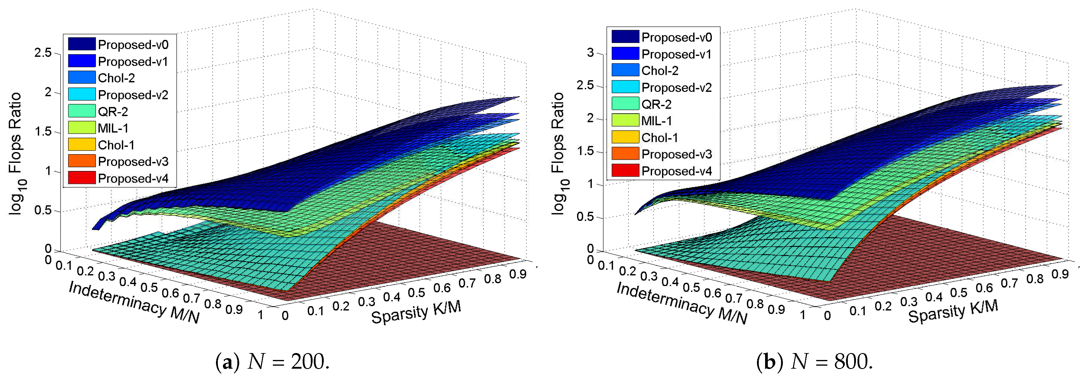
In Figure 7, we show ${log}_{10}\left(Flop{s}_{naive}(K,M,N)/Flop{s}_{imp}(K,M,N)\right)$ for two different N. Then in Figure 8 and Figure 9, we show the flops ratios of Chol-2 over Proposed-v0, Proposed-v1 and MIL-2, respectively, to compare flops among the efficient OMP implementations storing $\mathbf{G}$, and we also show the flops ratios of of QR-1 over Proposed-v2, Proposed-v3 and Proposed-v4, respectively, to compare flops among the efficient implementations that do not store $\mathbf{G}$. In Figure 8, we give the flops ratios as a function of the sparsity $K/M$ for the indeterminacies $M/N=0.1155$ and $M/N=0.5086$, respectively, while in Figure 9, we give the flops ratios as a function of the indeterminacy $M/N$ for the sparsities $K/M=0.1155$ and $K/M=0.5086$, respectively.

From Figure 7, it can be seen that the speedups in flop numbers of Proposed-v0, Proposed-v1, Chol-2, QR-2 and MIL-1 over Naive are obvious for almost all problem sizes. From Figure 8 and Figure 9, it can be seen that the speedups in flop numbers of Proposed-v0 and Proposed-v1 over Chol-2 and those of Proposed-v2 over QR-1 grow linearly with the increase of the sparsity $K/M$ for the two fixed indeterminacies $M/N$, and grow linearly with the increase of the indeterminacy $M/N$ for the two fixed sparsities $K/M$. On the other hand, with respect to QR-1, Proposed-v3 requires the similar number of flops and Proposed-v4 requires a little more flops, while as shown in Table 1, both Proposed-v3 and Proposed-v4 require less memories.

Figure 4 and Figure 7 indicate that Proposed-v1, Chol-2 and MIL-2 need less flops and more computational time, with respect to Proposed-v2, Proposed-v3 and QR-1, while Table 1 and Figure 2 of [24] also indicate that with respect to QR-1, Chol-2 and MIL-1 need less flops and more computational time. One possible reason for this phenomenon could be that the computational time is decided not only by the required flops, but also by the required operations for memory access. Specifically, this reason can partly explain why MIL-2 is obviously slower than Chol-2, since in the k-th iteration, MIL-2 needs to access $k^2$ memories in (38) to obtain the inverse of ${\mathbf{G}}_{{\mathbf{\Lambda }}_{k-1}}$, while Chol-2 only needs to access k memories in (20) to obtain the Cholesky factor of ${\mathbf{G}}_{{\mathbf{\Lambda }}_{k-1}}$.

In addition to the flops and the operations for memory access, the parallelizability of the OMP implementation can also affect the the computational time. When considering this factor, notice that the proposed five versions do not need any back-substitution in each iteration, and only include parallelizable matrix-vector products [45]. Contrarily, the existing Chol-1, Chol-2 and QR-2 usually solve triangular systems by back-substitutions [43], which are inherent serial processes unsuitable for parallel implementations [45]. It can be easily seen that Chol-1 and Chol-2 both need $\frac{3}{2}{k}^2$ multiplications and additions for the back-substitutions to solve 3 $k\times k$ triangular systems (17), (21) and (22), while QR-2 needs $k^2$ multiplications and additions for the back-substitutions to solve 2 $k\times k$ triangular systems (25) and (26).

5. Conclusions

Based on the efficient inverse Cholesky factorization proposed in [36], we propose an implementation of OMP (i.e., the proposed v0) and its four memory-saving versions (i.e., the proposed v1, v2, v3 and v4), and compare them with the existing ones. Among all the OMP implementations, the proposed v0 needs the least computational complexity, and is the fastest in the simulations for almost all problem sizes. The proposed v1, v2, v3 and v4 are all good tradeoffs between computational complexities/time and memory requirements. When only considering the efficient OMP implementations that spend $N^2$ memories to store $\mathbf{G}$ (i.e., the Gram matrix of the dictionary), the proposed v1 seems to be better than all the existing ones (i.e., QR-2, MIL-1, MIL-2, Chol-1 and Chol-2), since it needs less computational complexity, is usually faster in the simulations, and does not require more memories. When only considering the efficient OMP implementations that do not store $\mathbf{G}$, with respect to the only existing one (i.e., QR-1), the proposed v2 needs less computational complexity and a little more memories, while the proposed v3 needs the same complexity and less memories. Moreover, our simulations show that both the proposed v2 and v3 are faster than all the existing implementations for most problem sizes. Lastly, with respect to the naive OMP implementation that has the (known) minimum memory requirements, the proposed v4 only requires a little more memories, and needs much less computational time and complexities that are similar to those required by some existing efficient OMP implementations (e.g., the computational time of MIL-2 and Chol-2, and the complexities of QR-1). Thus the proposed v4 seems to be the best choice when we need an efficient implementation with the minimum memory requirements.

Our simulations show that the proposed five versions and the existing ones have nearly the same numerical errors. On the other hand, our simulations also show that some speedups in computational time or complexities of the proposed OMP implementations over the existing ones grow almost linearly with the increase of the sparsity $K/M$ or the indeterminacy $M/N$, e.g., the speedups in computational time of the proposed v0, v2 and v3 over Naive, those in complexities of the proposed v0 and v1 over Chol-2, and those in complexities of the proposed v2 over QR-1. Moreover, in each iteration, some existing efficient OMP implementations (e.g., Chol-1, Chol-2 and QR-2) solve triangular systems by back-substitutions (that are inherent serial processes unsuitable for parallel implementations), while the proposed five versions of OMP implementations do not need any back-substitution, and only include parallelizable matrix-vector products.