A Parallel Convolutional Neural Network for Pedestrian Detection

Abstract

Pedestrian detection is a crucial task in many vision-based applications, such as video surveillance, human activity analysis and autonomous driving. Recently, most of the existing pedestrian detection frameworks only focus on the detection accuracy or model parameters. However, how to balance the detection accuracy and model parameters, is still an open problem for the practical application of pedestrian detection. In this paper, we propose a parallel, lightweight framework for pedestrian detection, named ParallelNet. ParallelNet consists of four branches, each of them learns different high-level semantic features. We fused them into one feature map as the final feature representation. Subsequently, the Fire module, which includes Squeeze and Expand parts, is employed for reducing the model parameters. Here, we replace some convolution modules in the backbone with Fire modules. Finally, the focal loss is led into the ParallelNet for end-to-end training. Experimental results on the Caltech–Zhang dataset and KITTI dataset show that: Compared with the single-branch network, such as ResNet and SqueezeNet, ParallelNet has improved detection accuracy with fewer model parameters and lower Giga Floating Point Operations (GFLOPs).

1. Introduction

Pedestrian detection is an active research area in object detection [1]. The purpose of this study is to detect all pedestrians in each frame and locate their position, for applications in video surveillance [2], motion detection [3], intelligent transportation [4] and autonomous driving [5,6]. The development of pedestrian detection can be divided into two stages. The first is based on the feature engineering, with this type of method being consistent with “feature extractor + classifier” methods, such as Histogram of Oriented Gradient (HOG) + Support Vector Machines (SVM) [7], Integral Channel Features (ICF) + AdaBoost [8] and Deformable Part Model (DPM) + Latent Support Vector Machines (LatSVM) [9]. However, these methods still have limitations in their performance in engineering applications, particularly generalization performance [10]. The second is based on the neural network method. With the development of neural networks [11,12,13], general object detection algorithms are used in pedestrian detection, and can be further divided into two categories: Anchor-based and anchor-free. Anchor-based methods [14,15,16] mainly use anchors to generate proposal regions. This involves a large number of calculations but is able to achieve high detection accuracy. Anchor-free methods [16,17,18] take advantage of key point prediction, which can be more direct, avoiding a lot of IOU calculations. However, there remain some limitations to the performance of the overlap of key points. The method chosen for this paper was an anchor-based method and we will concentrate on this method from this point on.

In 2012, AlexNet turned out to be the winner of the ImageNet competition, reducing the error rate by almost 50%. Since then, the development of neural networks has made a qualitative leap. Networks such as VGGNet, GoogLeNet and ResNet have all been proposed, pushing deep learning to a new level. In recent years, in addition to the pursuit of network accuracy, more research has begun to focus on optimizing network structures by reducing model parameters and improving network computing efficiency. For example, SqueezeNet uses only 1/50 of the parameters of AlexNet to achieve the same level of accuracy. Analyzing the trend for the development of the backbone, along with the practical applications, it is clear that if we want to design an excellent backbone, we must consider both detection accuracy and model parameters.

Regarding detection accuracy, improving the robustness of feature representation in a network is crucial. Although various methods differ greatly, some networks are able to increase the depth of the network, improving its capacity for feature representation. However, increases in network depth will significantly increase the number of calculations and model parameters. Accordingly, we proposed the idea of building networks in parallel. With the goal of improving detection accuracy, we considered how to reduce the number of model parameters. Fortunately, research pioneers have discovered several effective methods for reducing model parameters and calculations, one of which, the Fire module, which includes Squeeze and Expand parts, was chosen for this research.

After analyzing the demand for pedestrian detection, this paper considers designing a backbone, which can effectively extract more accurate semantic features under limited parameter conditions and improve the detection accuracy of the model for pedestrian targets. Our main contributions are as follows:

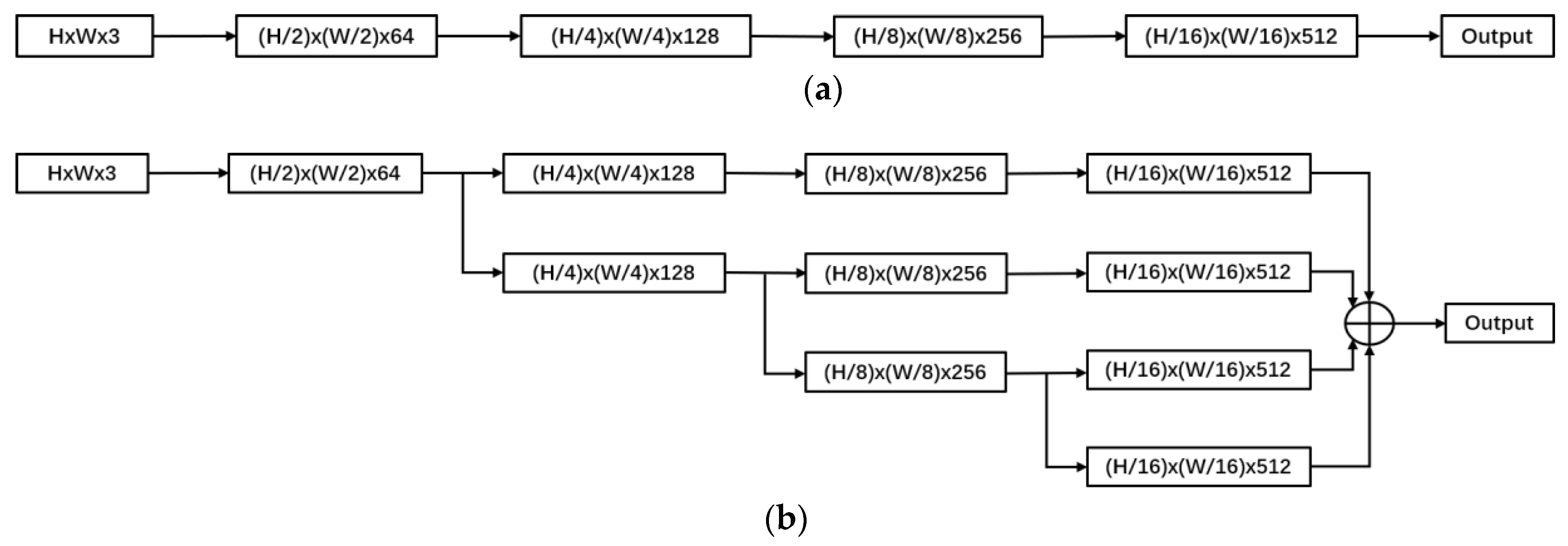
• We design a backbone with a parallel structure, which is called ParallelNet. It aims to improve the robustness of feature representation and detection accuracy.
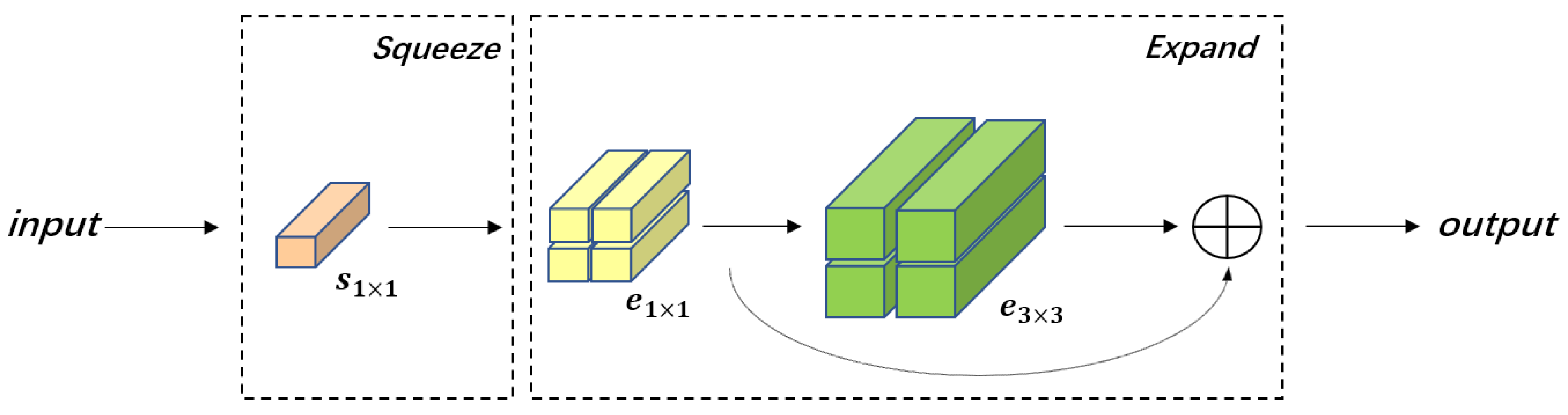
• A large number of Fire modules are employed, aiming to ensure accuracy while reducing the number of model parameters, with subsequent focal loss led into the ParallelNet for end-to-end training.
• We validate ParallelNet on the Caltech–Zhang and KITTI dataset, and compare the results with VGG16, ResNet50, ResNet101, SqueezeNet and SqueezeNet+. An ablation study was designed to verify the feasibility of the ParalleNet. In addition, to prevent the network from overfitting, we adopted data augmentation techniques, including random cropping and horizontal flipping.

The rest of the paper is organized as follows. We first review related works in Section 2. Then, we introduce the architecture of the ParallelNet and the detection head in Section 3. In Section 4, we report our experiments on the Caltech–Zhang and KITTI datasets, including details of experimental procedures and results. We conclude the paper in Section 5.

2. Related Works

2.1. Pedestrian Detection with Hand-Crafted Features

Before the advent of Convolutional Neural Networks (CNNs), a common method for pedestrian detection extracting hand-crafted features within a sliding window in all possible positions and ranges. The most significant methods are the VJ method proposed by Viola and Jones [19], and the HOG feature descriptor proposed by Dalal and Triggs [7]. The VJ method detects two consecutive frames, taking advantage of both pedestrian motion and appearance features, whereas the HOG feature descriptor uses gradient feature information to construct a histogram. Dollar et al. proposed ICF [8], which primarily constructs histograms based on feature information between different channels. Since then, a great number of excellent channel-based methods were proposed one after another [20,21,22,23]. These early works focused more on the design of feature descriptors, and mostly used SVM or Random Forest for classification. However, these methods continue to have limitations in engineering applications and limited generalization performance.

2.2. Pedestrian Detection with CNNs

In recent years, Convolutional Neural Network (CNN) has become the main method in general object detection [24,25,26], as well as pedestrian detection. Some pioneers apply the classic general object detection network to pedestrian detection. Zhang et al. [27] analyzed the reasons why Faster-RCNN did not perform well in pedestrian detection, and proposed to use Region Proposal Network (RPN) to generate candidate regions directly, and then use Boosted Forest for classification. Similarly, Li et al. [28] used two subnetworks to detect pedestrians of different scales on the basis of Faster-RCNN, and used a scale-aware weighting mechanism to reduce the impact of object scale on detection accuracy. Mao et al. [29] referred to the idea of aggregating channel features in the Aggregated Channel Features (ACF) method and improved the detection performance by adding channel feature information to the CNN network model.

Although these methods have made encouraging progress [30], experts continue to explore new ideas and methods. As pedestrian detection plays an increasingly important role in the application of autonomous driving systems, an increasing amount of research is being dedicated to dealing with more complex scenarios. Firstly, focusing on occluded pedestrians, Zhang et al. [31] characterized various occlusion modes by employing an attention mechanism across channels, and used the attention network as an additional component of the Faster-RCNN detector. Secondly, for the crowd, Wang et al. [32] proposed Repulsion loss to improve the robustness of the algorithm in crowd scenarios by reducing the weight of nonobject bounding box nearing the object bounding box. In addition, Shao et al. [33] proposed the crowd-oriented dataset, CrowdHuman. On average, each image contains about 23 pedestrian objects. Moreover, using CrowdHuman pretraining can also improve the performance of the algorithm on other datasets (such as Caltech and CityPersons). The third involves small-scale objects, the detection of which is crucial during the driving scenario as it can assist in giving users more timely warnings [34]. Song et al. [35] combined somatic topological line localization (TLL) and temporal feature aggregation, which works well for small-scale objects far away from the camera. Figure 1 shows the input examples of these three cases.

Ideally, the model will have a high energy efficiency and small size, so that the algorithm may be eventually used in mobile devices. Szegedy et al. [36] proposed replacing one 5 × 5 convolution kernel with two 3 × 3 convolution kernels, which both have the same receptive field; however, by doing so can deepen the network and reduce the calculation parameters. Subsequently, several novel convolution kernel design methods have been proposed in quick succession. Howard et al. [37] proposed Depthwise Separable Convolution, which integrates traditional convolution into two steps, namely depthwise convolution and pointwise convolution, which greatly improves the calculation efficiency [38,39,40]. Zhang et al. [41] introduced group convolution, then followed by an operation of channel shuffling. This method guarantees the exchange of information between different groups, and achieves the goal of improved calculation efficiency while maintaining accuracy. Iandola [42] proposed the Fire module, which consists of a Squeeze module and an Expand module, significantly reducing the number of parameters while improving the detection accuracy [43,44,45]. In this paper, we will adopt this innovative convolution module.

Essentially, all of these networks hope to detect the pedestrians more precisely with a small model size and real-time inference speed. In this research, we also commit to balancing the detection accuracy with model parameters.

2.3. Pedestrian Detection Benchmarks

Over the years, some datasets applied for video surveillance have been widely used, such as Daimler Pedestrian Detection Benchmark (DaimlerDB) [46], INRIA Person Dataset (INRIA) [7], ETH Pedestrian Dataset (ETH) [47], etc. However, in the past several years, for autonomous driving applications, many datasets have been proposed [48], including Caltech [49], KITTI [50], CityPersons [51], etc. These datasets are captured by onboard cameras while navigating through crowded areas and are widely used in various methods, in particular Caltech and KITTI. Zhang et al. [52] corrected the labeling errors in the Caltech dataset and provided a new sanitized version of annotations, which we call it Caltech–Zhang.

3. Architecture

In this section, we elaborate the architecture of ParallelNet and detection head. In Section 3.1, we introduce the strategies to improve the detection accuracy and reduce the model parameters. In Section 3.2, we introduce the detection strategies from localization, category and confidence score, respectively.

3.1. Architecture Design

3.1.1. Strategy 1: Parallel

Inspired by the human brain, experts hope to build a network similar to neural structures, hence the term “neural network”. In this type of network, each neuron is responsible for feature extraction. We obtain the weight of each neuron through suitable optimization methods, so that the output result is closest to the ground truth. Similarly, in a circuit structure, the principal objective is to obtain the ideal output by adjusting the resistance of the components. Analog circuit structures such as AlexNet and VGGNet can be regarded as series structures, where each layer of neurons is only connected to the previous layer of neurons, as shown in Figure 2a. If you increase the depth of the network, you may be able to increase the fitting ability of the network; however, it could also bring about complications such as overfitting, excessive calculation parameters, and vanishing gradient. These challenges are at the heart of the inspiration to design ParallelNet.

As shown in Figure 2b, we draw branches from the middle layer and extract features from the middle layer multiple times. Obviously, with the same network depth, the parallel structure network can extract more discriminative feature representation. This is similar to the principle of increasing network depth. However, it is not difficult for us to find that the more branches we introduce, the more calculation parameters of the network. Therefore, we need to further reduce the model parameters.

3.1.2. Strategy 2: Fire Model

The structure of the SqueezeNet network mentioned above is shown in Figure 3. It uses the Fire module to greatly reduce the number of model parameters while maintaining the detection accuracy. Therefore, we introduce the Fire module when optimizing the network structure. The Fire module is shown in Figure 4. Where we can see, the Fire module consists of two parts, “Squeeze” and “Expand”. The Squeeze part has several 1 × 1 convolutional kernels to reduce the dimensions of input. The Expand part has several 1 × 1 and 3 × 3 convolutional kernels to extract features and increase dimensions, respectively. In Figure 4, $s_{1 \times 1}$, $e_{1 \times 1}$ and $e_{3 \times 3}$ represent the numbers of kernels of each part.

Based on the above strategies, we have designed ParallelNet, whose structure is shown in Figure 5. Meanwhile, we take the Caltech–Zhang dataset as input and give the specific parameter settings of each layer in ParallelNet, as shown in

Table 1. The detailed parameters of each branch. (a) Branch-1; (b) Branch-2.; (c) Branch-3; (d) Branch-4.

(a)
Layer Name	Output Size	Size/Stride	$s_{1\times 1}$	$e_{1 \times 1}$	$e_{3\times 3}$
input	480 × 640 × 3	-	-	-	-
conv	240 × 320 × 64	3 × 3 × 64/2	-	-	-
pool1	120 × 160 × 64	3 × 3/2	-	-	-
fire1/fire2	120 × 160 × 64	-	16	64	64
pool2	60 × 80 × 64	3 × 3/2	-	-	-
fire3/fire4	60 × 80 × 128	-	32	128	128
pool3	30 × 40 × 128	3 × 3/2	-	-	-
fire5/fire6	30 × 40 × 192	-	48	192	192
fire7/fire8	30 × 40 × 256	-	64	256	256
pool4	15 × 20 × 256	3 × 3/2	-	-	-
fire9/fire10	15 × 20 × 384	-	96	384	384
fire11/fire12	15 × 20 × 512	-	128	512	512
feature map1	15 × 20 × 63	3 × 3 × 63/1	-	-	-
(b)
Layer Name	Output Size	Size/Stride	$s_{1\times 1}$	$e_{1\times 1}$	$e_{3\times 3}$
conv	120 × 160 × 128	3 × 3 × 128/2	-	-	-
pool1	60 × 80x128	3 × 3/2	-	-	-
fire1/fire2	60 × 80 × 128	-	32	128	128
pool2	30 × 40 × 128	3 × 3/2	-	-	-
fire3/fire4	30 × 40 × 192	-	48	192	192
fire5/fire6	30 × 40 × 256	-	64	256	256
pool3	15 × 20 × 256	3 × 3/2	-	-	-
fire7/fire8	15 × 20 × 384	-	96	384	384
fire9/fire10	15 × 20 × 512	-	128	512	512
feature map2	15 × 20 × 63	3 × 3 × 63/1	-	-	-
(c)
Layer Name	Output Size	Size/Stride	$s_{1\times 1}$	$e_{1\times 1}$	$e_{3\times 3}$
conv	60 × 80 × 128	3 × 3 × 128/2	-	-	-
pool1	30 × 40 × 128	3 × 3/2	-	-	-
fire1	30 × 40 × 192	-	48	192	192
fire2	30 × 40 × 192	-	48	192	192
fire3	30 × 40 × 256	-	64	256	256
fire4	30 × 40 × 256	-	64	256	256
pool2	15 × 20 × 256	3 × 3/2	-	-	-
fire1/fire2	15 × 20 × 384	-	96	384	384
fire3/fire4	15 × 20 × 512	-	128	512	512
feature map3	15 × 20 × 63	3 × 3 × 63/1	-	-	-
(d)
Layer Name	Output Size	Size/Stride	$s_{1\times 1}$	$e_{1\times 1}$	$e_{3\times 3}$
conv	30 × 40 × 256	3 × 3 × 256/2	-	-	-
pool1	15 × 20 × 256	3 × 3/2	-	-	-
fire1/fire2	15 × 20 × 384	-	96	384	384
fire3/fire4	15 × 20 × 512	-	128	512	512
feature map4	15 × 20 × 63	3 × 3 × 63/1	-	-	-

. It is not difficult to find that ParallelNet has used a large number of Fire modules in each branch, and the output of each branch is a feature map with a size of 15 × 20 × 63.

3.2. Detection Head

As mentioned in the previous section, each branch will output a feature map. We added the corresponding pixels of the four feature maps to get one feature map, and fed it into the detection network. Before explaining the detection process, Figure 6 roughly illustrates the detection process. From Figure 6, we can see that the feature map includes three parts: localization, category and confidence score.

3.2.1. Bounding Box Loss

How do we get the coordinates of the bounding box? Assume that the size of the feature map is $H\times W$. Here, H and W are the height and width, respectively. $K$ is the number of anchors. In the detection stage, we carried out the following steps:

• Sliding the window to get the coordinate of the anchor, denoted as $\left({\widehat{x}}_i,{\widehat{y}}_j,{\widehat{\omega }}_k,{\widehat{h}}_k\right)$. Here, $\mathrm{i}\in \left[1,W\right]$, $j\in \left[1,H\right]$, $k\in \left[1,K\right]$. the ground truth is known, denoted as $\left(x_i^G,y_j^G,{\omega }_k^G,h_k^G\right)$.
• Calculating the offset, denoted as $\left(\delta x_{ijk},\delta y_{ijk},\delta {\omega }_{ijk},\delta h_{ijk}\right)$, by encoding Equation (1). After a period of training and optimization, the offset convergences to the threshold, which means that the predicted bounding box is close to the ground truth.
• Calculating the coordinate of the predicted bounding box, denoted as $\left(x_i^P,y_j^P,{\omega }_k^P,h_k^P\right)$, by decoding Equation (2).

$$\begin{gathered} \delta x_{ijk}^G=\left(x_i^G-{\widehat{x}}_i\right)/{\widehat{\omega }}_k \\ \delta y_{ijk}^G=\left(y_j^G-{\widehat{x}}_j\right)/{\widehat{h}}_k \\ \delta {\omega }_{ijk}^G=\log \left({\omega }_k^G/{\widehat{\omega }}_k\right) \\ \delta h_{ijk}^G=\log \left(h_k^G/{\widehat{h}}_k\right) \end{gathered}$$

(1)

$$\begin{gathered} x_i^P={\widehat{x}}_{\mathrm{i}}+{\widehat{\omega }}_k\delta x_{ijk} \\ {y}_j^P={\widehat{y}}_j+{\widehat{h}}_k\delta y_{ijk} \\ {\omega }_k^P={\widehat{\omega }}_{k}exp\left(\delta {\omega }_{ijk}\right) \\ {h}_k^P={\widehat{h}}_{k}exp\left(\delta h_{ijk}\right) \end{gathered}$$

(2)

Consequently, the loss function of the bounding box is to optimize the offset between predict bounding box and ground truth bounding box, as:

$$l_{bbox}=\frac{{\lambda }_{bbox}}{N_{obj}}{\displaystyle \sum }_{i=1}^W{\displaystyle \sum }_{j=1}^H{\displaystyle \sum }_{k=1}^K{I}_{ijk}[{\left(\delta x_{ijk}-\delta x_{ijk}^G\right)}^2+{\left(\delta y_{ijk}-\delta y_{ijk}^G\right)}^2+{\left(\delta {\omega }_{ijk}-\delta {\omega }_{ijk}^G\right)}^2+[{\left(\delta h_{ijk}-\delta h_{ijk}^G\right)}^2]$$

(3)

where $W,H,K$ are the width, height and number of channels of the feature map, respectively; $N_{obj}$ is the number of objects; for anchor located at $\left(i,j,k\right)$, if it contains object, $I_{ijk}=1$, else $I_{ijk}=0$; ${\lambda }_{bbox}$ is the coefficient.

3.2.2. Classification Loss

In terms of classification, the pedestrian detection problem is a binary classification problem. The most commonly used loss function for binary classification problems is the cross-entropy loss function, as:

$$l_{class}=\frac{{\lambda }_{class}}{N_{obj}}{\displaystyle \sum }_{i=1}^W{\displaystyle \sum }_{j=1}^H{\displaystyle \sum }_{k=1}^K{\displaystyle \sum }_{c=1}^C{I}_{ijk}{l}_c\log \left(p_c\right)$$

(4)

where $C$ is the number of categories; $p_c$ is the output of detection head, which represents the probability that a bounding box contains an object; $l_cϵ\left\{0,1\right\}$, which is the ground truth;${\lambda }_{class}$ is the coefficient.

However, reviewing ParallelNet, we use four branches to extract features separately. Obviously, we can extract more discriminative feature representation but it also means that we may be disturbed by more background information. This is not conducive to the robustness of training. In addition, in the driving scene, the background information is complex, and there is a problem of extreme foreground-background class imbalance. Therefore, we used focal loss [53] as the classification loss function, as:

$$l_{class}=\frac{{\lambda }_{class}}{N_{obj}}{\displaystyle \sum }_{i=1}^W{\displaystyle \sum }_{j=1}^H{\displaystyle \sum }_{k=1}^K{\displaystyle \sum }_{c=1}^C{I}_{ijk}{\alpha }_c{\left(1-p_c\right)}^{\gamma }\left(-\log \left(p_c\right)\right)l_c$$

(5)

where $\gamma$ is the focusing parameter, which smoothly downweight the rate for easy examples. $\alpha$ is the balance parameter, which is used to balance proportions of positive instances and negative instances.

3.2.3. Confidence Score Loss

In terms of confidence score, we define the confidence score as $p_c\times IOU$. The $IOU$ is the intersection-over union between the predicted bounding box and the ground truth bounding box. Similarly, for the loss function of confidence score, we take the negative examples into account, as:

$$l_{conf}={\displaystyle \sum }_{i=1}^W{\displaystyle \sum }_{j=1}^H{\displaystyle \sum }_{k=1}^K(\frac{{\lambda }_{conf}^{+}}{N_{obj}}{I}_{ijk}{\left(IO{U}^{+}\right)}^2+\frac{{\lambda }_{conf}^{-}}{WHK-N_{obj}}\left(1-I_{ijk}\right){\left(IO{U}^{-}\right)}^2$$

(6)

where $IO{U}^{+}$ is the IOU for positive instance and ground truth; $IO{U}^{-}$ is the IOU for negative instance and ground truth; ${\lambda }_{conf}^{+}$, ${\lambda }_{conf}^{-}$ are the coefficients.

4. Experimental Results

In this part, we will specifically introduce our experimental procedures and results to evaluate the method in this paper. First, we will introduce the basic experimental setup and implementation details. Then, the results of the ParalleNet on Caltech and KITTI datasets will be compared with VGG16, ResNet50, ResNet101, SqueezeNet and SqueezeNet+. At the same time, we further verify the feasibility of the parallel network through ablation experiments. Finally, we will explain some of the tricks applied during the experiment and show the detection results.

4.1. Experiment Settings

4.1.1. Datasets

The two datasets used in this paper are Caltech–Zhang and KITTI. Based on the original Caltech pedestrian dataset, Zhang et al. corrected several types of errors in the existing annotations, such as misalignments, missing annotations (false negatives), false annotations (false positives) and the inconsistent use of “ignore” regions. Caltech–Zhang has a total of 5039 images, and the input image size is 480 × 640.

KITTI is a benchmark that is designed with autonomous driving for the tasks of stereo, optical flow, visual odometry/SLAM (Simultaneous Localization and Mapping) and 3D object detection. There are 7481 pictures in total the size of the input image is 1242 × 375, including several kinds of labels, such as car, truck, pedestrian, tram and so on. However, we only detect the pedestrian category.

4.1.2. Training Details

In the experiment, we train the model on NVIDIA 2080Ti GPU, and randomly divide datasets into two equal parts as the training set and the validation set. We set the batch size to 20 and the number of anchors to nine; we used Stochastic Gradient Descent (SGD) with momentum to optimize the loss function during training, where the momentum was set to 0.9; we set the initial learning rate to 0.001, and each after 10,000 steps, it is decayed in half; ${\lambda }_{class}$= 1, ${\lambda }_{conf}^{+}$= 75, ${\lambda }_{conf}^{-}$= 100, ${\lambda }_{bbox}$= 5, ${\alpha }_1$= 0.25, ${\alpha }_0$= 0.75, $\gamma$ = 2; the final stage used Non-Maximum Suppression (NMS to filter the bounding boxes.

4.2. Experiments

4.2.1. Comparative Experiments

We experimented on Caltech–Zhang and KITTI datasets, respectively. In addition to the ParallelNet proposed in this paper, we also conducted experiments with the same settings on the backbones of VGG16, ResNet50, ResNet101, SqueezeNet and SqueezeNet+.Then fed the result into the same detection network, just as described in Section 3.2. The experimental results are shown in

Table 2. Comparison results of ParallelNet with some most commonly used backbone evaluated on Caltech–Zhang and KITTI dataset. AP is the average precise, which is used to measure the detection accuracy; FPS is the number of images processed per second, which represents the detection speed; # Param is the number of model elements, the lower is better; GFLOPs is the FLOPs (floating point of operations) per image, which also the lower is better. (a) On Caltech–Zhang; (b) On KITTI.

(a)
Backbone	AP (%)	FPS	# Param (MB)	GFLOPs
VGG16	51.39	21.11	17.91	75.44
ResNet50	52.54	27.78	9.11	39.63
ResNet101	53.22	24.31	15.48	70.86
SqueezeNet	48.90	43.48	2.02	6.68
SqueezeNet+	53.44	30.30	6.98	50.42
PrallelNet	54.61	35.71	7.54	17.73
(b)
Backbone	AP (%)	FPS	# Param (MB)	GFLOPs
VGG16	72.89	18.65	17.91	117.69
ResNet50	73.05	25.00	9.11	60.97
ResNet101	74.19	22.50	15.48	107.71
SqueezeNet	68.66	37.04	2.02	10.34
SqueezeNet+	73.90	29.41	6.98	77.11
PrallelNet	77.90	32.26	7.54	27.35

. It should be pointed out that SqueezeNet+ deepens the network on the basis of the SqueezeNet, and uses a 7 × 7 convolution kernel to increase the receptive field.

Compared to VGG16, ResNet50 and ResNet101, ParallelNet achieved 35.71 FPS on Caltech–Zhang and 32.26 FPS on KITTI. The good performance on detection speed benefits from the employment of the Fire module. Simultaneously, although the architecture of ParallelNet seems complicated, the Fire module greatly reduces the model parameters and GFLOPs, which can also be seen from the experimental results.

Compared to SqueezeNet and SqueezeNet+, which also employed the Fire module, ParallelNet achieved the best performance on detection accuracy, 54.61% AP on Caltech–Zhang and 77.9% AP on KITTI. Unfortunately, the detection speed of ParallelNet is not as fast as SqueezeNet. This is not difficult to understand, for that ParallelNet constructs branches in parallel to extract more feature representation, which will inevitably increase the GFLOPs. However, from the experimental results, we can also find that the detection speed of ParallelNet is better than that of SqueezeNet+. This shows that the “parallel connection” compared to the "series connection", well balances the detection accuracy and model parameters. This also provides a new idea for the construction of the backbone.

4.2.2. Ablation Study

In the structure of Figure 5, we introduced parallel branches and finally got the output of four equal-sized feature maps. In the next experiment, we increase the number of parallel branches in turn, and compare the results on the Caltech–Zhang dataset, just as shown in

Table 3. In the table, 1-branch means that no parallel branch is introduced, but only one branch; 2-branches means that one parallel branch is introduced, a total of 2 branches; and so on.

Backbone	AP (%)	FPS	# Param (MB)	GFLOPs
1-branch	48.90	43.48	2.02	6.68
2-branches	50.08	43.55	3.65	10.05
3-branches	52.03	37.02	5.41	14.85
4-branches	54.61	35.71	7.54	17.73

.

Judging from the experimental results, the detection results of each additional branch are improved. However, with the improvement of detection accuracy, the detection speed has decreased. It is not to find the reason. As the number of branches increases, the model becomes more complex, which means that we need more time and resources to train the network. This makes it impossible to balance detection accuracy and detection speed, which means we cannot increase the number of parallel branches indefinitely. Therefore, under comprehensive considerations, 4-branches was selected as the final solution.

4.3. Results

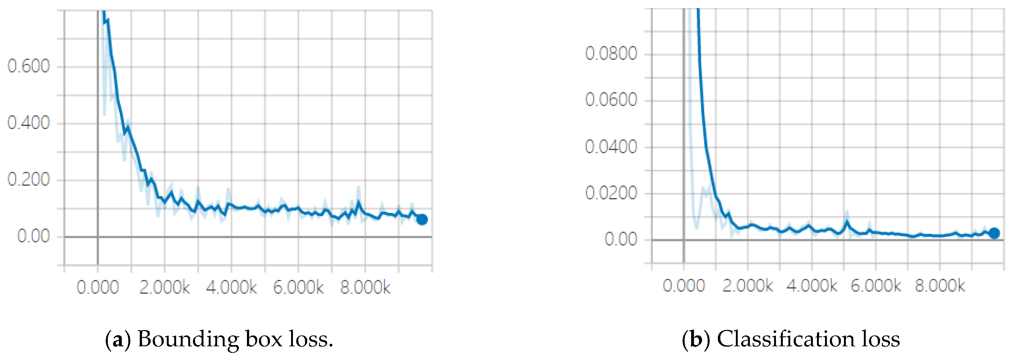
4.3.1. Training Results

In the training stage, we have given a quantization of experimental results. In this part, we will give some intuitive, graphical results. As the settings described in Section 4.1.2, ParallelNet was trained for 9700 steps. Figure 7 shows the loss for the training along with the number of training steps. The loss graphs, including bounding box loss, classification loss and confidence score loss, all converge toward a small value. The total loss converges from 35.2 to about 0.4. It proves that the model has been fully trained.

4.3.2. Testing Results

In the testing stage, some detection results are shown in Figure 8. We have randomly selected some representative instances. Taking Figure 8a as an example, the two pictures in the first column show that the model performs well on the single and small-scaled; the two in the second column show that, no matter from the side or the back of the pedestrian, the model can give correct detection results; and the two in the last column show some more complex situations, such as occluded pedestrian and multiscaled pedestrians. Figure 8b also illustrates a fraction of detection results on the KITTI dataset.

4.3.3. Tricks

Except for the experiment procedures aforementioned, we also introduce several tricks, just as the following:

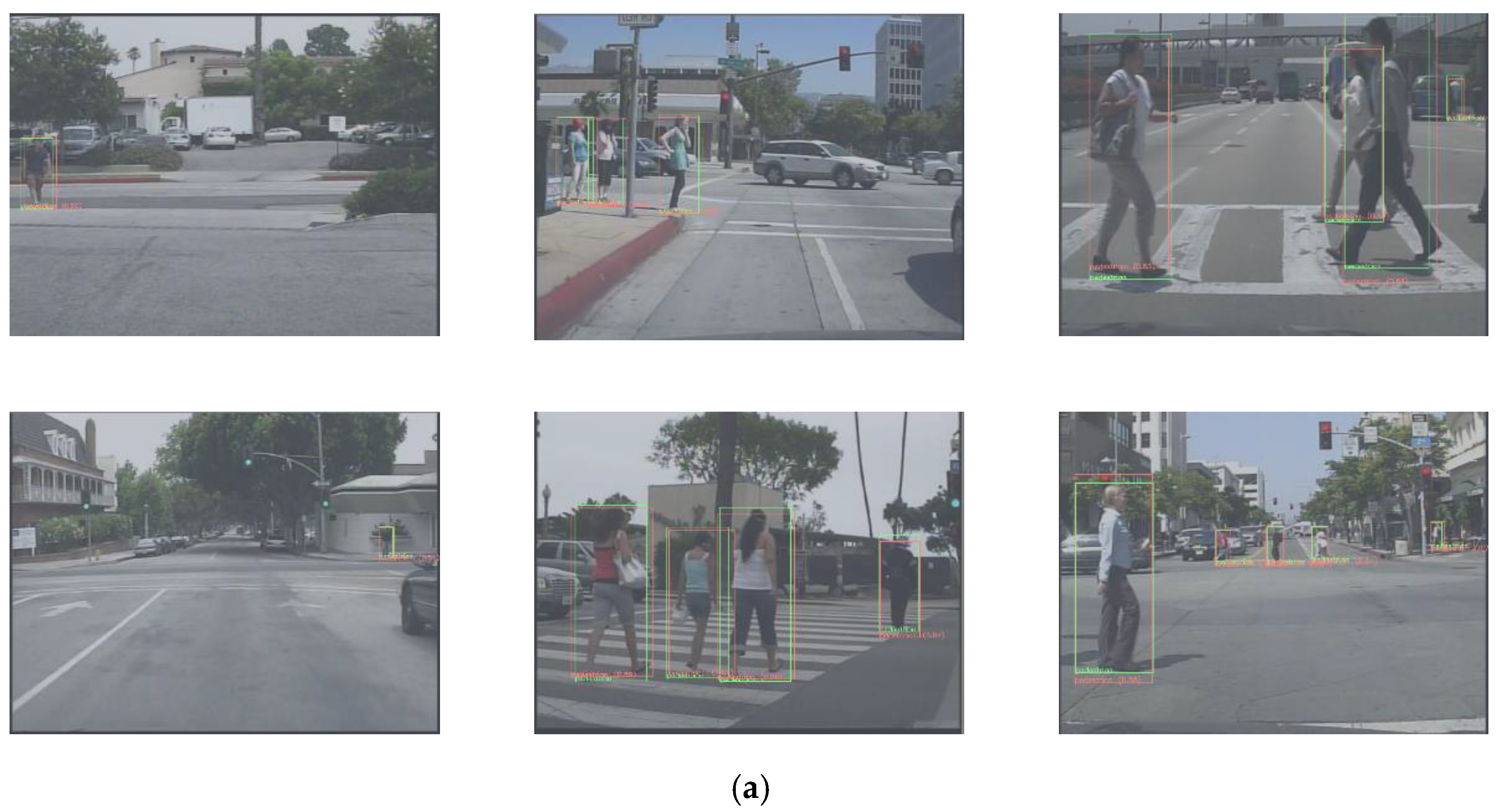
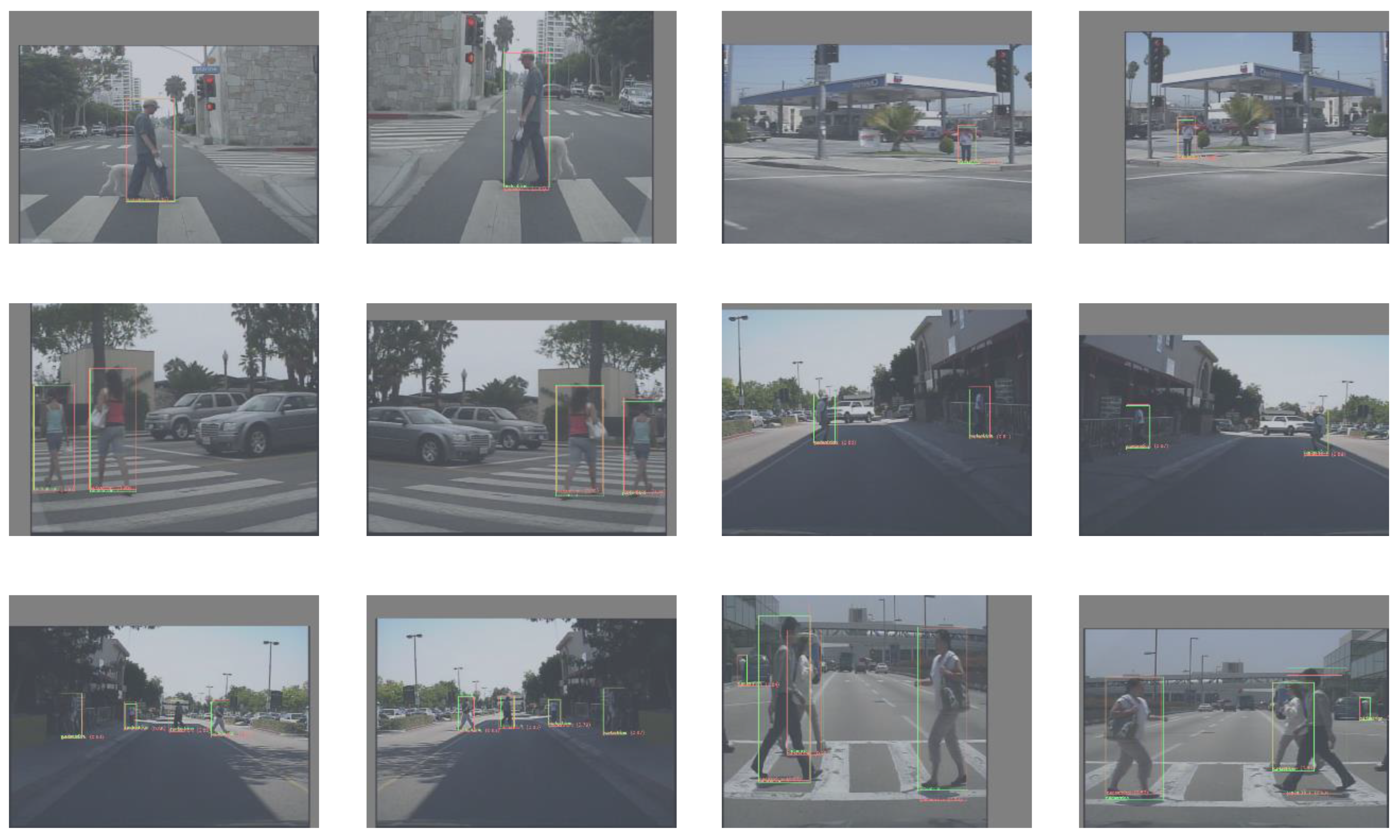
• In order to prevent the network from overfitting, an L2 loss is added to the total loss function. In addition, data augmentation techniques are used, including random cropping and horizontal flipping. Figure 9 shows some detection examples after data augmentation.
• As mentioned above, our ParallelNet will output four feature maps of equal size, which need to be merged into one feature map when inputting the detection head. There are several alternative fusion methods, including concatenating by channel, add by pixel, average by pixel and maximum by pixel. Through experiments, the detection accuracy of several methods is similar, but the calculation of the pixel-by-pixel method is less, so the method of adding by pixel is finally selected.

5. Conclusions

This paper proposed ParallelNet, a backbone composed of four branches in parallel, applied for the pedestrian detection task. To satisfy the requirement of both high accuracy and small model size, we further applied the Fire module in the network. Subsequently, in the detection stage, a convolutional layer is added to generate the detection bounding box, which also reduces the model parameter. Moreover, the focal loss is applied to ameliorate the problem of extreme foreground-background class imbalance. Experimental results on the Caltech–Zhang dataset and KITTI dataset show that, compared with the one-branch network, such as ResNet, SqueezeNet and so on, ParallelNet has improved detection accuracy with fewer model parameters and lower GFLOPs. In addition, compared to the method of increasing the depth of the network, the idea of constructing the network in parallel is better in both improving the detection accuracy and reducing parameter. In the future work, we will apply this idea to other excellent lightweight networks, such as MobileNet, ShuffleNet and MixNet proposed recently.

References

1. Hasan, I.; Liao, S.; Li, J.; Akram, S.U.; Shao, L. Pedestrian Detection: The Elephant In The Room. arXiv 2020, arXiv:2003.08799. [Google Scholar]
2. Lee, J.H.; Choi, J.-S.; Jeon, E.S.; Kim, Y.G.; Le, T.T.; Shin, K.Y.; Lee, H.C.; Park, K.R. Robust pedestrian detection by combining visible and thermal infrared cameras. Sensors 2015, 15, 10580–10615. [Google Scholar] [CrossRef] [PubMed] [Green Version]
3. Martínez, M.A.; Martínez, J.L.; Morales, J. Motion detection from mobile robots with fuzzy threshold selection in consecutive 2D Laser scans. Electronics 2015, 4, 82–93. [Google Scholar] [CrossRef]
4. Liu, K.; Wang, W.; Wang, J. Pedestrian detection with LiDAR point clouds based on single template matching. Electronics 2019, 8, 780. [Google Scholar] [CrossRef] [Green Version]
5. Ball, J.E.; Tang, B. Machine Learning and Embedded Computing in Advanced Driver Assistance Systems (ADAS). Electronics 2019, 8, 748. [Google Scholar] [CrossRef] [Green Version]
6. Barba-Guaman, L.; Eugenio Naranjo, J.; Ortiz, A. Deep Learning Framework for Vehicle and Pedestrian Detection in Rural Roads on an Embedded GPU. Electronics 2020, 9, 589. [Google Scholar] [CrossRef] [Green Version]
7. Dalal, N.; Triggs, B. Histograms of oriented gradients for human detection. In Proceedings of the IEEE Computer Society Conference on Computer Vision and Pattern Recognition, San Diego, CA, USA, 20–25 June 2005; pp. 886–893. [Google Scholar]
8. Dollár, P.; Tu, Z.; Perona, P.; Belongie, S. Integral channel features. In Proceedings of the British Machine Vision Conference, London, UK, 7–10 September 2009. [Google Scholar]
9. Felzenszwalb, P.; McAllester, D.; Ramanan, D. A discriminatively trained, multiscale, deformable part model. In Proceedings of the IEEE Conference on Computer Vision and Pattern Recognition, Anchorage, AK, USA, 23–28 June 2008; pp. 1–8. [Google Scholar]
10. Sun, T.; Fang, W.; Chen, W.; Yao, Y.; Bi, F.; Wu, B. High-Resolution Image Inpainting Based on Multi-Scale Neural Network. Electronics 2019, 8, 1370. [Google Scholar] [CrossRef] [Green Version]
11. Wang, X.; Hua, X.; Xiao, F.; Li, Y.; Hu, X.; Sun, P. Multi-object detection in traffic scenes based on improved SSD. Electronics 2018, 7, 302. [Google Scholar] [CrossRef] [Green Version]
12. Xu, D.; Wu, Y. Improved YOLO-V3 with DenseNet for Multi-Scale Remote Sensing Target Detection. Sensors 2020, 20, 4276. [Google Scholar] [CrossRef]
13. Zhao, L.; Li, S. Object Detection Algorithm Based on Improved YOLOv3. Electronics 2020, 9, 537. [Google Scholar] [CrossRef] [Green Version]
14. Wei, H.; Kehtarnavaz, N. Semi-supervised faster RCNN-based person detection and load classification for far field video surveillance. Mach. Learn. Knowl. Extr. 2019, 1, 756–767. [Google Scholar] [CrossRef] [Green Version]
15. Nguyen, K.; Huynh, N.T.; Nguyen, P.C.; Nguyen, K.-D.; Vo, N.D.; Nguyen, T.V. Detecting Objects from Space: An Evaluation of Deep-Learning Modern Approaches. Electronics 2020, 9, 583. [Google Scholar] [CrossRef] [Green Version]
16. Liu, W.; Liao, S.; Ren, W.; Hu, W.; Yu, Y. High-level semantic feature detection: A new perspective for pedestrian detection. In Proceedings of the IEEE Conference on Computer Vision and Pattern Recognition, Long Beach, CA, USA, 16–20 June 2019; pp. 5187–5196. [Google Scholar]
17. Tian, Z.; Shen, C.; Chen, H.; He, T. Fcos: Fully convolutional one-stage object detection. In Proceedings of the IEEE International Conference on Computer Vision, Seoul, Korea, 27–28 October 2019; pp. 9627–9636. [Google Scholar]
18. Zhu, C.; He, Y.; Savvides, M. Feature selective anchor-free module for single-shot object detection. In Proceedings of the IEEE Conference on Computer Vision and Pattern Recognition, Long Beach, CA, USA, 16–20 June 2019; pp. 840–849. [Google Scholar]
19. Viola, P.; Jones, M.J.; Snow, D. Detecting pedestrians using patterns of motion and appearance. Int. J. Comput. Vis. 2005, 63, 153–161. [Google Scholar] [CrossRef]
20. Dollár, P.; Appel, R.; Belongie, S.; Perona, P. Fast feature pyramids for object detection. IEEE Trans. Pattern Anal. Mach. Intell. 2014, 36, 1532–1545. [Google Scholar] [CrossRef] [PubMed] [Green Version]
21. Zhang, S.; Benenson, R.; Schiele, B. Filtered channel features for pedestrian detection. In Proceedings of the IEEE Conference on Computer Vision and Pattern Recognition, Boston, MA, USA, 7–12 June 2015; p. 4. [Google Scholar]
22. Kwon, S.; Park, T. Channel-Based Network for Fast Object Detection of 3D LiDAR. Electronics 2020, 9, 1122. [Google Scholar] [CrossRef]
23. Yang, B.; Yan, J.; Lei, Z.; Li, S.Z. Aggregate channel features for multi-view face detection. In Proceedings of the IEEE International Joint Conference on Biometrics, Clearwater, FL, USA, 29 September–2 October 2014; pp. 1–8. [Google Scholar]
24. Liu, W.; Anguelov, D.; Erhan, D.; Szegedy, C.; Reed, S.; Fu, C.-Y.; Berg, A.C. Ssd: Single shot multibox detector. In Proceedings of the European Conference on Computer Vision, Amsterdam, The Netherlands, 10–16 October 2016; pp. 21–37. [Google Scholar]
25. Redmon, J.; Divvala, S.; Girshick, R.; Farhadi, A. You only look once: Unified, real-time object detection. In Proceedings of the IEEE Conference on Computer Vision and Pattern Recognition, Seattle, WA, USA, 27–30 June 2016; pp. 779–788. [Google Scholar]
26. Ren, S.; He, K.; Girshick, R.; Sun, J. Faster R-CNN: Towards Real-Time Object Detection with Region Proposal Networks. IEEE Trans. Pattern Anal. Mach. Intell. 2017, 1137–1149. [Google Scholar] [CrossRef] [PubMed] [Green Version]
27. Zhang, L.; Lin, L.; Liang, X.; He, K. Is faster R-CNN doing well for pedestrian detection? In Proceedings of the European Conference on Computer Vision, Amsterdam, The Netherlands, 8–16 October 2016; pp. 443–457. [Google Scholar]
28. Li, J.; Liang, X.; Shen, S.; Xu, T.; Feng, J.; Yan, S. Scale-aware fast R-CNN for pedestrian detection. IEEE Trans. Multimed. 2017, 20, 985–996. [Google Scholar] [CrossRef] [Green Version]
29. Mao, J.; Xiao, T.; Jiang, Y.; Cao, Z. What can help pedestrian detection? In Proceedings of the IEEE Conference on Computer Vision and Pattern Recognition, Honolulu, HI, USA, 21–26 October 2017; pp. 3127–3136. [Google Scholar]
30. Zhang, S.; Benenson, R.; Omran, M.; Hosang, J.; Schiele, B. Towards reaching human performance in pedestrian detection. IEEE Trans. Pattern Anal. Mach. Intell. 2017, 40, 973–986. [Google Scholar] [CrossRef]
31. Zhang, S.; Yang, J.; Schiele, B. Occluded pedestrian detection through guided attention in cnns. In Proceedings of the IEEE Conference on Computer Vision and Pattern Recognition, Salt Lake City, UT, USA, 18–23 June 2018; pp. 6995–7003. [Google Scholar]
32. Wang, X.; Xiao, T.; Jiang, Y.; Shao, S.; Sun, J.; Shen, C. Repulsion loss: Detecting pedestrians in a crowd. In Proceedings of the IEEE Conference on Computer Vision and Pattern Recognition, Salt Lake City, UT, USA, 18–23 June 2018; pp. 7774–7783. [Google Scholar]
33. Shao, S.; Zhao, Z.; Li, B.; Xiao, T.; Yu, G.; Zhang, X.; Sun, J. Crowdhuman: A benchmark for detecting human in a crowd. arXiv 2018, arXiv:1805.00123. [Google Scholar]
34. Zhang, X.; Cheng, L.; Li, B.; Hu, H.-M. Too far to see? Not really!—Pedestrian detection with scale-aware localization policy. IEEE Trans. Image Process. 2018, 27, 3703–3715. [Google Scholar] [CrossRef] [Green Version]
35. Song, T.; Sun, L.; Xie, D.; Sun, H.; Pu, S. Small-scale pedestrian detection based on topological line localization and temporal feature aggregation. In Proceedings of the European Conference on Computer Vision, Munich, Bavaria, Germany, 8–14 September 2018; pp. 536–551. [Google Scholar]
36. Szegedy, C.; Liu, W.; Jia, Y.; Sermanet, P.; Reed, S.; Anguelov, D.; Erhan, D.; Vanhoucke, V.; Rabinovich, A. Going deeper with convolutions. In Proceedings of the IEEE Conference on Computer Vision and Pattern Recognition, Columbus, OH, USA, 24–27 June 2014; pp. 1–9. [Google Scholar]
37. Howard, A.G.; Zhu, M.; Chen, B.; Kalenichenko, D.; Wang, W.; Weyand, T.; Andreetto, M.; Adam, H. Mobilenets: Efficient convolutional neural networks for mobile vision applications. arXiv 2017, arXiv:1704.04861. [Google Scholar]
38. Kim, W.; Jung, W.-S.; Choi, H.K. Lightweight driver monitoring system based on multi-task mobilenets. Sensors 2019, 19, 3200. [Google Scholar] [CrossRef] [PubMed] [Green Version]
39. Lee, D.-H. Fully Convolutional Single-Crop Siamese Networks for Real-Time Visual Object Tracking. Electronics 2019, 8, 1084. [Google Scholar] [CrossRef] [Green Version]
40. Liu, B.; Zou, D.; Feng, L.; Feng, S.; Fu, P.; Li, J. An fpga-based cnn accelerator integrating depthwise separable convolution. Electronics 2019, 8, 281. [Google Scholar] [CrossRef] [Green Version]
41. Zhang, X.; Zhou, X.; Lin, M.; Sun, J. Shufflenet: An extremely efficient convolutional neural network for mobile devices. In Proceedings of the IEEE Conference on Computer Vision and Pattern Recognition, Salt Lake City, UT, USA, 18–23 June 2018; pp. 6848–6856. [Google Scholar]
42. Iandola, F.N.; Han, S.; Moskewicz, M.W.; Ashraf, K.; Dally, W.J.; Keutzer, K. SqueezeNet: AlexNet-level accuracy with 50x fewer parameters and < 0.5 MB model size. arXiv 2016, arXiv:1602.07360. [Google Scholar]
43. Wu, B.; Iandola, F.; Jin, P.H.; Keutzer, K. Squeezedet: Unified, small, low power fully convolutional neural networks for real-time object detection for autonomous driving. In Proceedings of the IEEE Conference on Computer Vision and Pattern Recognition Workshops, Honolulu, HI, USA, 21–26 July 2017; pp. 129–137. [Google Scholar]
44. Li, C.; Wei, X.; Yu, H.; Guo, J.; Tang, X.; Zhang, Y. An Enhanced SqueezeNet Based Network for Real-Time Road-Object Segmentation. In Proceedings of the 2019 IEEE Symposium Series on Computational Intelligence (SSCI), Xiamen, China, 6–9 December 2019; pp. 1214–1218. [Google Scholar]
45. Sun, W.; Zhang, Z.; Huang, J. RobNet: Real-time road-object 3D point cloud segmentation based on SqueezeNet and cyclic CRF. Soft Comput. 2019, 24, 5805–5818. [Google Scholar] [CrossRef]
46. Flohr, F.; Gavrila, D. Daimler Pedestrian Segmentation Benchmark Dataset. In Proceedings of the British Machine Vision Conference, Bristol, UK, 9–13 September 2013. [Google Scholar]
47. Ess, A.; Leibe, B.; Van Gool, L. Depth and appearance for mobile scene analysis. In Proceedings of the IEEE International Conference on Computer Vision, Minneapolis, MN, USA, 17–22 June 2007; pp. 1–8. [Google Scholar]
48. Dominguez-Sanchez, A.; Cazorla, M.; Orts-Escolano, S. A new dataset and performance evaluation of a region-based cnn for urban object detection. Electronics 2018, 7, 301. [Google Scholar] [CrossRef] [Green Version]
49. Dollár, P.; Wojek, C.; Schiele, B.; Perona, P. Pedestrian detection: A benchmark. In Proceedings of the IEEE Conference on Computer Vision and Pattern Recognition, Miami Beach, FL, USA, 20–25 June 2009; pp. 304–311. [Google Scholar]
50. Geiger, A.; Lenz, P.; Urtasun, R. Are we ready for autonomous driving. In Proceedings of the IEEE Computer Vision and Pattern Recognition, Providence, RI, USA, 16–21 June 2012; pp. 3354–3361. [Google Scholar]
51. Zhang, S.; Benenson, R.; Schiele, B. Citypersons: A diverse dataset for pedestrian detection. In Proceedings of the IEEE Conference on Computer Vision and Pattern Recognition, Honolulu, HI, USA, 21–26 July 2017; pp. 3213–3221. [Google Scholar]
52. Zhang, S.; Benenson, R.; Omran, M.; Hosang, J.; Schiele, B. How far are we from solving pedestrian detection? In Proceedings of the IEEE Conference on Computer Vision and Pattern Recognition, Seattle, WA, USA, 27–30 June 2016; pp. 1259–1267. [Google Scholar]
53. Lin, T.-Y.; Goyal, P.; Girshick, R.; He, K.; Dollár, P. Focal loss for dense object detection. In Proceedings of the IEEE International Conference on Computer Vision, Venice, Italy, 22–29 October 2017; pp. 2980–2988. [Google Scholar]
Figure 1. (a) is a case where the pedestrian is partially occluded. (b) is a case where there are many pedestrians in a frame of image. (c) is a case where the pedestrian has a quite small size or long distance. These images and ground truth bounding boxes are from the Caltech–Zhang pedestrian dataset.
Electronics 09 01478 g001
Figure 2. The size of the input image is H × W × 3, where H is the height, W is the width, and 3 is the number of channels. Here, the form of a circuit is used to represent the network structure, where (a) represents a neural network with a series structure, and (b) represents a neural network with a parallel structure.
Electronics 09 01478 g002
Figure 3. The structure of SqueezeNet. The last 2 layers are to fine-tune the model, which do not appear in the initial training. So, we use a dotted box to represent the last 2 layers.
Electronics 09 01478 g003
Figure 4. The structure of the Fire module from input to output.
Electronics 09 01478 g004
Figure 5. The structure of ParallelNet. It consists of 4 branches in parallel, and each branch generates a feature map of equal size. In the follow-up process, the 4 feature maps will be fused into one feature map.
Electronics 09 01478 g005
Figure 6. If the number of anchors in the experiment is assumed to be K , the dimension of the prediction tensor will be K ( 2 + 1 + 4 ) . Among them, 2 represents the number of categories, that is, pedestrian/not pedestrian, 1 represents confidence score, and 4 represents the coordinates of the bounding box.
Electronics 09 01478 g006
Figure 7. Loss graphs of the training stage, taking the experiment on the Caltech–Zhang as an example. Where, (a) is the bounding box loss; (b) is the classification loss; (c) is the confidence score loss; (d) is the total loss, which is the sum of previous three loss functions.
Electronics 09 01478 g007aElectronics 09 01478 g007b
Figure 8. The detection results of images randomly selected for several situations. The green bounding box is the true value, and the red is the detection box. (a) Caltech–Zhang; (b) KITTI.
Electronics 09 01478 g008aElectronics 09 01478 g008b
Figure 9. Take the results on Caltech–Zhang as an example, two adjacent pictures are the detection output of the same input after data augmentation.
Electronics 09 01478 g009