1. Introduction
In recent years, algorithmic trading has drawn more and more attention in the field of reinforcement learning and finance. There are many classical reinforcement learning algorithms being used in the financial sector. Jeong & Kim use deep Q-learning to improve financial trading decisions [
1]. They use a deep neural network to predict the number of shares to trade and propose a transfer learning algorithm to prevent overfitting. Deep deterministic policy gradient (DDPG) is explored to find the best trading strategies in complex dynamic stock markets [
2]. Optimistic and pessimistic reinforcement learning is applied for stock portfolio allocation. Reference [
3] using asynchronous advantage actor-aritic (A3C) and deep Q-network (DQN) with stacked denoising autoencoders (SDAEs) gets better results than Buy & Hold strategy and original algorithms. Zhipeng Liang et al. implement policy gradient (PG), PPO, and DDPG in portfolio management [
4]. In their experiments, PG is more desirable than PPO and DDPG, although both of them are more advanced.
In addition to different algorithms, research objects are many and various. Kai Lei et al. combine gated recurrent unit (GRU) and attention mechanism with reinforcement learning to improve single stock trading decision making [
5]. A constrained portfolio trading system is set up using a particle swarm algorithm and recurrent reinforcement learning [
6]. The system yields a better efficient frontier than mean-variance based portfolios. Reinforcement learning agents are also used for trading financial indices [
7]. David W. Lu uses recurrent reinforcement learning and long short term memory (LSTM) to trade foreign exchange [
8]. From the above, we can see reinforcement learning can be applied to many financial assets.
However, most of the work in this field does not pay much attention to the training data set. It is well known that deep learning needs plenty of data to train to get a satisfactory result. And reinforcement learning requires even more data to achieve an acceptable result. Reference [
8] uses over ten million frames to train the DQN model to reach and even exceed human level across 57 Atari games. In the financial field, the daily-candle data is not sufficient to train a reinforcement learning model. The amount of minute-candle data is enormous, but high-frequency trading like trading once per minute is not suitable for the great majority of the individual investors. And intraday trading is not allowed for common stocks in the A-share market. Therefore, we propose a data augmentation method to address the problem. Minute-candle data is used to train the model, and then the model can be applied to daily assets trading, which is similar to transfer learning. Training set and test set have similar characteristics and different categories.
This study not only has research significance and application meaning in financial algorithmic trading but also provides a novel data augmentation method in reinforcement learning training of daily financial assets trading. The main contributions of this paper can be summarized as follows:
We propose an original data augmentation approach that can enlarge the scale of the training dataset a hundred times as before by using minute-candle data to replace daily data. By this means, adequate data is available for training reinforcement learning model, leading to a satisfactory result.
The data augmentation method mentioned above is not suitable for all financial assets. We provide an access mechanism based on skewness and kurtosis to select proper stocks that can be traded using the proposed algorithm.
The experiments show that the proposed model using the data augmentation method can get decent returns compared with Buy & Hold strategy in the dataset the model has not seen before. This indicates our model learns some useful law from minute-candle data and then applies it to daily stock trading.
The remaining parts of this paper are organized as follows.
Section 2 describes the preliminaries and reviews the background on reinforcement learning as well as data augmentation.
Section 3 describes the data augmentation based reinforcement learning (DARL) framework and details the concrete algorithms.
Section 4 provides experimental settings, results, and evaluation.
Section 5 concludes this paper and points out some promising future extensions.
2. Preliminaries and Background
In this section, we first present the introduction to algorithmic trading. Thereafter, reinforcement learning (RL), policy-based reinforcement learning, and Q-Learning are introduced. Finally, we discuss data augmentation and two important statistics.
2.1. Algorithmic Trading
Algorithmic trading is a process for executing orders utilizing automated and pre-programmed trading instructions to account for variables such as price, timing, and volume. An algorithm is a set of directions for solving a problem. Computer algorithms send small portions of the full order to the market over time.
Algorithmic trading uses complex formulas, combined with mathematical models and human oversight, to make decisions to buy or sell financial securities on an exchange. Algorithmic trading can be used in various situations, including order execution, arbitrage, and trend trading strategies. Reinforcement learning is suitable for continuous decision-making in the algorithmic trading scenario and can be easily extended into an online learning version.
2.2. Reinforcement Learning
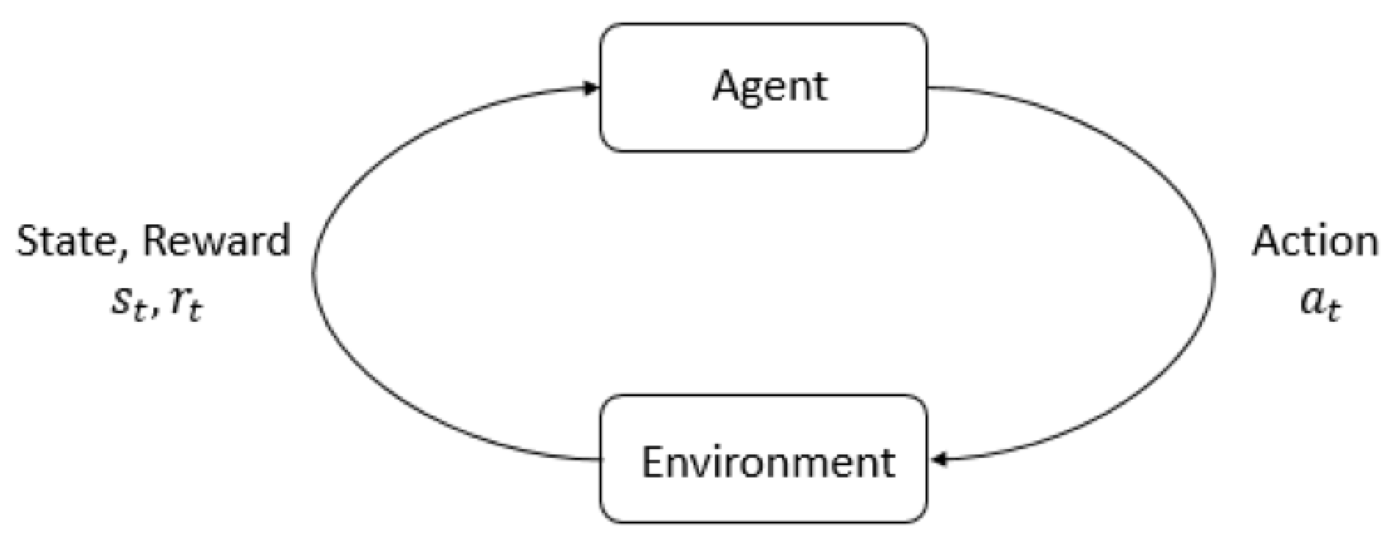
The main characters of reinforcement learning are the agent and the environment. The environment is the world that the agent lives in and interacts with. It changes when the agent acts on it, but may also change on its own. At every step of interaction, the agent sees an observation of the state of the world and then decides on an action to take. It also perceives a reward signal from the environment, a number that tells it how good or bad the current world state is. The goal of the agent is to maximize its cumulative reward, called return. Reinforcement learning enables the agent to learn behaviors to achieve its goal.
Figure 1 demonstrates the interaction loop between agent and environment.
A policy is a rule used by an agent to decide what actions to take. It can be deterministic, and denoted by
:
or it may be stochastic, and denoted by
:
A trajectory
is a sequence of states and actions in the world,
The reward function
R is critically important in reinforcement learning. It depends on the current state of the world, the action just taken, and the next state of the world:
2.3. Policy Optimization and Q-Learning
There are two main approaches to representing and training agents with model-free RL: policy optimization and Q-Learning.
Policy Optimization. Methods in this family represent a policy explicitly as . They optimize the parameters either directly by gradient ascent on the performance objective , or indirectly, by maximizing local approximations of . This optimization is almost always performed on-policy, which means that each update only uses data collected while acting according to the most recent version of the policy.
A couple of examples of policy optimization methods are:
A2C/A3C [
9], which performs gradient ascent to maximize performance directly,
and PPO [
10], whose updates indirectly maximize performance, by instead maximizing a surrogate objective function which gives a conservative estimate for how much
will change as a result of the update.
Q-Learning. Methods in this family learn an approximator
for the optimal action-value function,
. Typically they use an objective function based on the Bellman equation. This optimization is almost always performed off-policy, which means that each update can use data collected at any point during training, regardless of how the agent was chosen to explore the environment when the data was obtained. The corresponding policy is obtained via the connection between
and
: the actions taken by the Q-learning agent are given by
Examples of Q-learning methods include
DQN [
11], a classic which substantially launched the field of deep RL,
and C51 [
12], a variant that learns a distribution over return whose expectation is
.
The primary strength of policy optimization methods is that they are principled in the sense that you directly optimize for the thing you want. This tends to make them stable and reliable. By contrast, Q-learning methods only indirectly optimize agent performance by training to satisfy a self-consistency equation. It is less stable. But, Q-learning methods gain the advantage of being substantially more sample efficient when they work, because they can reuse data more effectively than policy optimization techniques.
Policy optimization and Q-learning are not incompatible (and under some circumstances, it turns out equivalent [
13]), and there exist a range of algorithms that live in between the two extremes. Algorithms that live on this spectrum can carefully trade-off between the strengths and weaknesses of either side.
DDPG [
14] is an algorithm that concurrently learns a deterministic policy and a Q-function by using each to improve the other.
SAC [
15] is a variant that uses stochastic policies, entropy regularization, and a few other tricks to stabilize learning and score higher than DDPG on standard benchmarks.
2.4. Data Augmentation
Data augmentation is a data-space solution to the problem of limited data. It encompasses a suite of techniques that enhance the size and quality of training dataset such that a better deep learning model can be built using them [
16]. There are lots of augmentation algorithms in image datasets, such as geometric transformation, color space augmentations, kernel filters, mixing images, random erasing, etc. Some algorithms can also be used in reinforcement learning, like adversarial training, generative adversarial networks (GAN), neural style transfer, and meta-learning.
Model-free RL can suffer from limited data if the environment cannot provide infinite training data, such as in the financial field. To address the shortcoming, model-based RL can synthesize a model of the world from experience [
17]. Using an internal model to reason about the future, the agent can seek positive outcomes while avoiding the adverse consequences of trial-and-error in the real environment. Pengqian Yu et al. take advantage of GAN to generate synthetic market data [
18]. They train a recurrent GAN using historical asset data to produce realistic multi-dimensional time series.
Data augmentation method is based on fractal theory. Almost all fractals are at least partially self-similar. This means that a part of the fractal is identical to the entire fractal itself except smaller. The stock data also has such a fractal nature. We can think of stock data as a continuous timing chart, and minute-candle data is part of the overall timing chart. Any keen observer of the market would be aware that the patterns seen on the intra-day charts of 1-min, 5- min, 10-min intervals and so on are very similar to the patterns seen on the daily, weekly, monthly, or even quarterly charts. Distributional self-similarity is found in the financial time series [
19]. Therefore, the minute-candle data maintains the distribution properties of the daily-candle data. It is reasonable to expand the daily-candle data with the minute-candle data.
2.5. Skewness and Kurtosis
Skewness is usually described as a measure of a dataset’s symmetry. A perfectly symmetrical data set will have a skewness of 0. The normal distribution has a skewness of 0. Skewness is defined as:
where
n is the sample size,
is the
ith
X value,
is the average and
s is the sample standard deviation. The skewness is referred to as the third standardized central moment for the probability model.
Kurtosis measures the tail-heaviness of the distribution. Kurtosis is defined as:
Kurtosis is referred to as the fourth standardized central moment for the probability model.
3. The Proposed DARL
In this section, the proposed data augmentation reinforcement learning model is demonstrated. Firstly, we present the financial asset environment in our model. It contains observation of the reinforcement learning algorithm and feedback of specific state and action. Secondly, we introduce the PPO and SAC used by our model. They can represent state-of-the-art policy-based algorithms and actor-critic algorithms, respectively. Finally, we describe the data augmentation method used in our model.
3.1. Financial Asset Environment
A standard reinforcement learning environment usually contains state, action, reward, and done or not. For financial assets, our state (namely, the algorithm observation) includes time, open, high, low, and close [
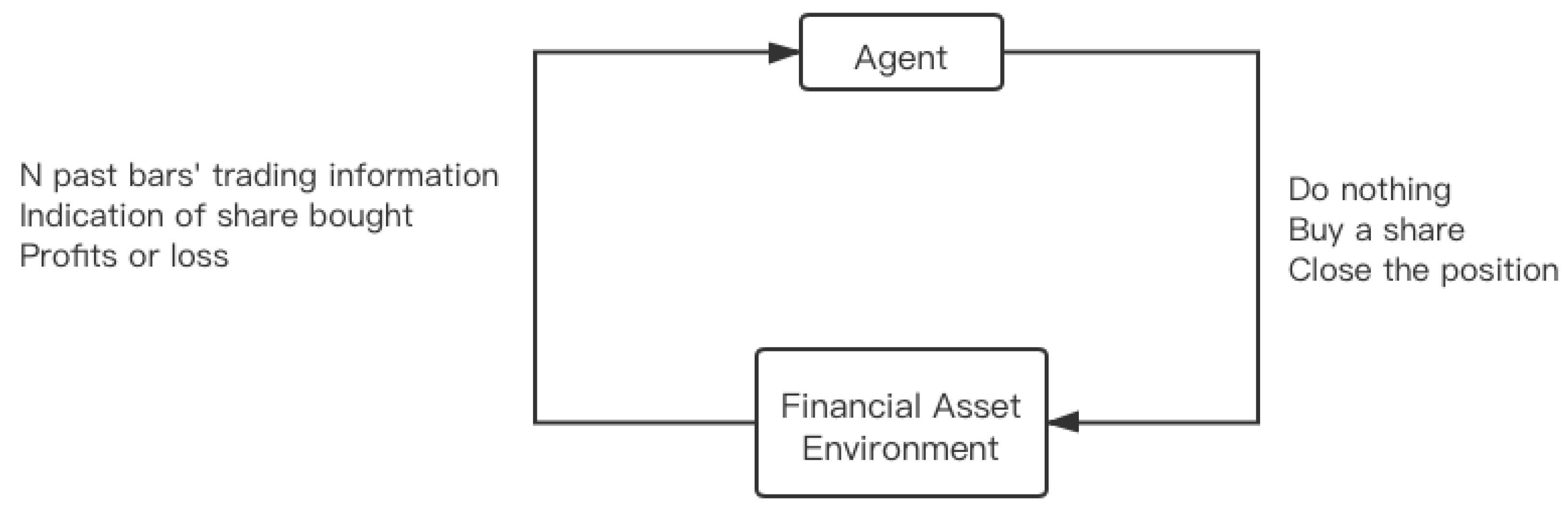
20]. The open price is the price at the beginning of the minute or day, high is the maximum price during the interval, low is the minimum price, and the close price is the last price of the time interval. Every time interval is called a bar and allows us to have an idea of price movement within the interval. In our model, the algorithm observation includes three parts:
N past bars, where each has open, high, low, and close prices
An indication that the share was bought some time ago (only one share at a time will be possible)
Profits or loss that we currently have from our current position (the share bought)
At every step, the agent can take one of the following actions:
Do nothing: skip the bar without taking an action
Buy a share: if the agent has already got the share, nothing will be bought; otherwise, we will pay the commission (0.1% by default)
Close the position: if we do not have a previously purchased share, nothing will happen; otherwise, we will pay the commission of the trade
According to the definition, the agent looks N past bars’ trading information from the environment. Our model is like a higher-order Markov chain model [
21]. Higher-order Markov chain models remember more than one-step historical information. Additional history can have predictive value.
The reward that the agent receives can be split into multiple steps during the ownership of the share. In that case, the reward on every step will be equal to the last bar’s movement. On the other hand, the agent will receive the reward only after the close action and receive the full reward at once. At first sight, both variants should have the same final result, but maybe with different convergence speeds. However, we find that the latter approach gets a more stable training result and is more likely to gain high reward. Therefore, we use the second approach in the final model.
Figure 2 shows the interaction between our agent and the financial asset environment.
3.2. Primary Algorithm Introduction
PPO and SAC are two state-of-the-art reinforcement learning algorithms. They are used to verify the effectiveness of the data augmentation method. Details of the two algorithms are as follows:
3.2.1. Proximal Policy Optimization
PPO is motivated by the same question of trust region policy optimization (TRPO) [
22]. How can we take the biggest possible improvement step on a policy using the data we currently have, without stepping so far that we accidentally cause performance collapse? TRPO tries to solve this problem with a complicated second-order method. PPO is a family of first-order methods that use a few other tricks to keep new policies close to old.
PPO updates policies via
typically taking multiple steps of (usually minibatch) SGD to maximize the objective. Here
L is given by
in which
is a (small) hyperparameter which roughly says how far away the new policy is allowed to go from the old.
There is another simplified version of this objective:
where
Clipping serves as a regularizer by removing incentives for the policy to change dramatically. The hyperparameter corresponds to how far away the new policy can go from the old while still profiting the objective.
3.2.2. Soft Actor-Critic
SAC is an algorithm that optimizes a stochastic policy in an off-policy way. A central feature of SAC is entropy regularization. The policy is trained to maximize a trade-off between expected return and entropy, a randomness measure in the policy. Increasing entropy results in more exploration, which can accelerate learning later on. It can also prevent the policy from prematurely converging to a bad local optimum.
Entropy is a quantity which says how random a random variable is. Let
x be a random variable with probability mass
P. The entropy
H of
x is computed from its distribution
P according to
In entropy-regularized reinforcement learning, the agent gets bonus reward at each timestep. This changes the RL problem to:
where
is the trade-off coefficient. The policy of SAC should, in each state, act to maximize the expected future return plus expected future entropy.
Original SAC is for continuous action settings and not applicable to discrete action settings. To deal with discrete action settings of our financial asset, we use an alternative version of the SAC algorithm that is suitable for discrete actions. It is competitive with other model-free state-of-the-art RL algorithms [
23].
3.3. Data Augmentation Method
Data augmentation techniques enlarge the original dataset to improve results and avoid overfitting. It is often used in deep learning, especially in image datasets. We now present our proposed method: We use minute-candle data instead of the daily-candle data to train the reinforcement learning model. Minute-candle data and daily-candle data are both composed of four tuples, including open, high, low, and close prices. One trading day contains hundreds of minutes of trading. The training dataset is augmented vastly. And the characteristics of minute-candle data and daily-candle data are similar. In DARL, we use the model trained on minute-candle data to guide the daily stock trading. DARL provides a paradigm for using minute-candle data set to train the agent that guides daily trading.
However, the minute-candle dataset is not the same as daily trading data, which results in that not all financial assets are suitable for this kind of trading. To resolve the problem, we propose an access mechanism based on skewness and kurtosis to select stocks that can be traded in this way. The detail of the access mechanism is discussed in
Section 4.
4. Experiments and Results
In this section, we describe our experiments and results in three aspects. Firstly, the dataset and trading environments are introduced. Secondly, our model and trading agents are presented in detail. At last, we analyze the experimental results and discuss other relevant aspects of the framework.
4.1. Dataset and Trading Environments
As mentioned in
Section 3, our training dataset is in units of a minute. We choose Yandex company stock for 2016 as a training dataset. There are 130k lines in the form of
Table 1.
In the training and testing process, transaction costs are set as 0.1% (buy and sell are the same). For testing assets, we select two kinds of stocks from the A-share market. For rising stocks, our model can get higher returns. For declining stocks, our model can make less loss, or even create some profit. We have applied DARL to thirty different financial assets. Eleven of them meet the requirements of the access mechanism based on skewness and kurtosis. The eleven assets all get satisfactory results using our agents. And for the rest of the assets that can not satisfy the two requirements simultaneously, most of them perform poorly in our experiments. From the eleven assets, we choose three typical stocks. They are YZGF (603886.SH), KLY (002821.SZ), NDSD (300750.SZ) from the Tushare database [
24]. The stocks from IPO (Initial Public Offering) to 12 June 2020 are dealt with in our experiment. Owing to different starting times, we can test our agents in diverse a time period to verify their robustness. The period we choose is after 2016 to avoid overlapping with the training dataset.
We only use the minute-candle data as training set and use target stock’s daily data as testing set without using target stock data for training, which is like zero-shot meta learning.
4.2. Trading Agents
The reinforcement learning framework we use is SLM-Lab [
25], a software framework for reproducible RL research. It enables easy development of RL algorithms using modular components and file-based configuration. In our experiments, we use DQN, PPO, and SAC to train the trading agents. Their setting details are introduced as follows.
4.2.1. Deep Q-Learning
Our DQN agent is initialized with four normalized inputs (open, high, low, close price), two hidden fully-connected layers (512-512), and three outputs (buy, hold, sell). We use 6 million steps to train DQN and use 0.1 million steps as max replay buffer size. By using SLM-Lab, one experiment is a trial in the framework. And it contains four concurrent sessions. Each session includes the same algorithm structure and different initialized random parameters. They are run independently, thus getting different experimental results.
Figure 3 shows the DQN trial graph that is a collection of 4 sessions. The trial graph takes the mean of sessions and plots an error envelop using standard deviation. It helps visualize the averaged performance of different sessions that have multiple random seeds. From
Figure 3, we can see a rising trend of average returns during 6 million training steps. The difference between the four sessions is not very huge.
4.2.2. Proximal Policy Optimization
Our PPO agent has the same inputs, outputs, and network structure as the DQN agent. We use 10 million steps to train the PPO agent.
Figure 4 demonstrates that the PPO agent in 4 sessions gets stable and substantial return increase during 10 million steps. It seems like an ideal agent to guide daily stock trading in our experiment.
4.2.3. Soft Actor-Critic
Our SAC agent’s inputs, outputs, and network structure are identical to the PPO agent. 2 million steps are used to train the SAC agent, and its max replay buffer size is 1 million steps.
Figure 5 suggests that the SAC agent’s four sessions vary considerably, based on its target to maximize entropy. On average, the SAC agent obtains satisfactory returns. Therefore, we can choose the best session model to guide another stock trading.
4.3. Results and Discussions
The annualized return (AR) and the sharp ratio (SR) are used as evaluation metrics. Annualized return can put different periods into the same scale, which is benefit to compare various stock returns using different agents. Sharp ratio is a kind of risk-adjusted return. It is computed as
, where
is the return,
is the risk-free rate, and
is the standard deviation of excess return.
Table 2 shows the AR and SR for each selected asset. Three reinforcement learning algorithms are evaluated: DQN, PPO, and SAC. The baseline of trading strategy is buy and hold (B&H). To compare with B&H, we set the risk-free rate to 0. Sharp ratio is a relative metric, which is applied to compare risk-adjusted returns of different trading strategies.
4.3.1. General Evaluations
From
Table 2, we can see that PPO is more stable than the other two agents because its AR and SR outperform the B&H strategy consistently. On the contrary to training results, DQN and SAC often surpass the B&H strategy in AR and always exceed the B&H strategy in SR. Besides, DQN or SAC sometimes gets the highest SR among all strategies, which means the largest risk-adjusted return. It is worth noting that the stock and period of our training dataset is entirely different from that of the testing dataset. Therefore, we can conclude that the excess return of agents can be attributed to the inherent market law found by the agents. And the law does not change with stock and period. In conclusion, PPO is a stable algorithm in our experiment; on the other hand, DQN and SAC can get higher AR and SR at times.
4.3.2. Algorithm Comparison
Figure 6 illustrates the details of the profit curves of Stock YZGF and NDSD.
Figure 6a shows all three agents can make profit even in a declining trend, although we have not allowed short operation in trading due to the unique characteristics of the A-share market. From
Figure 6, we can see that PPO and SAC trace the B&H trend on the whole. And DQN has its own strategy, which sometimes leads to lower returns but always gets higher risk-adjusted returns. Furthermore, SAC sometimes gets higher returns than PPO due to its high intrinsic entropy. As a consequence of high entropy, the SAC agent can take some novel actions and decrease overfitting to the training dataset. In general, using minute-candle data as training data does contribute to better algorithmic trading even in different stocks and periods.
4.3.3. Access Mechanism
The agents trained on the minute-candle data in our experiment can work well on some daily stocks, but not on all. Therefore, an access mechanism is used to select stocks suitable for our agents. The mechanism is based on two numerical characteristics, skewness and kurtosis. Skewness is the degree of distortion from the symmetrical bell curve or the normal distribution. It measures the lack of symmetry in the data distribution. Kurtosis is all about the tails of the distribution. It is used to describe the extreme values in one versus the other tail. Skewness and kurtosis of eight stocks or ETFs (Exchange Traded Funds) are shown in
Table 3. Besides the three stocks discussed above, the five assets are ZGHL (513050.SH), HSZS (159920.SZ), TGYY (300347.SZ), AEYK (300015.SZ) and HLSN (600585.SH). Close prices of the eight assets from 2017 are used to calculate skewness and kurtosis. We find that when
and
, our agents perform well. Positive skewness means the tail on the right side of the distribution is longer or fatter, and positive kurtosis means distribution is longer or tails are fatter. In other words, prices are made up of more low prices close to the mean and less high prices far from the mean. Besides, more extreme prices exist in the distribution compared with the normal distribution. There are more chances for our agents buying stocks at lower prices and selling stocks at extremely high prices.
5. Conclusions and Future Work
In this study, a data augmentation based reinforcement learning (DARL) framework is proposed to address the deficiency of training data in financial deep reinforcement learning. Financial minute-candle data is used to train the agents, and then the agents can guide daily financial assets trading. To select suitable financial assets, an access mechanism based on skewness and kurtosis is put forward. RL algorithms, such as DQN, PPO, and SAC, are utilized to verify the framework’s effectiveness. The experimental results show that the PPO agent can outperform B&H strategy consistently in AR and SR. DQN and SAC agents surpass B&H strategy in SR. Thus, it can be seen that our framework works on daily stock trading even in different stocks and periods from the training dataset.
While the proposed framework has been verified effectively, there are still some directions worth studying in the future. We put forward a new paradigm to address the training data sparseness problem. Based on this, historical data of investment targets or stock data with similar market capitalization and volatility can be combined with transfer learning to get higher performance in future research.
Author Contributions
Conceptualization, Y.Y. and J.Y.; methodology, W.W. and Y.Y.; software W.W.; writing—original draft preparation, W.W., Y.Y. and J.Y.; writing—review and editing, W.W. and J.Y. All authors have read and agreed to the published version of the manuscript.
Funding
This work is supported by the National Natural Science Foundation of China (No.91118002).
Conflicts of Interest
The authors declare no conflict of interest.
References
- Jeong, G.; Kim, H.Y. Improving financial trading decisions using deep Q-learning: Predicting the number of shares, action strategies, and transfer learning. Expert Syst. Appl. 2019, 117, 125–138. [Google Scholar] [CrossRef]
- Li, X.; Li, Y.; Zhan, Y.; Liu, X.-Y. Optimistic bull or pessimistic bear: Adaptive deep reinforcement learning for stock portfolio allocation. arXiv 2019, arXiv:1907.01503. [Google Scholar]
- Li, Y.; Zheng, W.; Zheng, Z. Deep robust reinforcement learning for practical algorithmic trading. IEEE Access 2019, 7, 108014–108022. [Google Scholar] [CrossRef]
- Liang, Z.; Chen, H.; Zhu, J.; Jiang, K.; Li, Y. Adversarial deep reinforcement learning in portfolio management. arXiv 2018, arXiv:1808.09940. [Google Scholar]
- Lei, K.; Zhang, B.; Li, Y.; Yang, M.; Shen, Y. Time-driven feature-aware jointly deep reinforcement learning for financial signal representation and algorithmic trading. Expert Syst. Appl. 2020, 140, 112872. [Google Scholar] [CrossRef]
- Almahdi, S.; Yang, S.Y. A constrained portfolio trading system using particle swarm algorithm and recurrent reinforcement learning. Expert Syst. Appl. 2019, 130, 145–156. [Google Scholar] [CrossRef]
- Pendharkar, P.C.; Cusatis, P. Trading financial indices with reinforcement learning agents. Expert Syst. Appl. 2018, 103, 1–13. [Google Scholar] [CrossRef]
- Hessel, M.; Modayil, J.; Van Hasselt, H.; Schaul, T.; Ostrovski, G.; Dabney, W.; Horgan, D.; Piot, B.; Azar, M.; Silver, D. Rainbow: Combining improvements in deep reinforcement learning. In Proceedings of the Thirty-Second AAAI Conference on Artificial Intelligence, New Orleans, LO, USA, 2–7 February 2018. [Google Scholar]
- Mnih, V.; Badia, A.P.; Mirza, M.; Graves, A.; Lillicrap, T.; Harley, T.; Silver, D.; Kavukcuoglu, K. Asynchronous methods for deep reinforcement learning. In Proceedings of the International Conference on Machine Learning, New York, NY, USA, 19–24 June 2016; pp. 1928–1937. [Google Scholar]
- Schulman, J.; Wolski, F.; Dhariwal, P.; Radford, A.; Klimov, O. Proximal policy optimization algorithms. arXiv 2017, arXiv:1707.0634. [Google Scholar]
- Mnih, V.; Kavukcuoglu, K.; Silver, D.; Graves, A.; Antonoglou, I.; Wierstra, D.; Riedmiller, M. Playing atari with deep reinforcement learning. arXiv 2013, arXiv:1312.5602. [Google Scholar]
- Bellemare, M.G.; Dabney, W.; Munos, R. A distributional perspective on reinforcement learning. arXiv 2017, arXiv:1707.06887. [Google Scholar]
- Schulman, J.; Chen, X.; Abbeel, P. Equivalence between policy gradients and soft q-learning. arXiv 2017, arXiv:1704.06440. [Google Scholar]
- Lillicrap, T.P.; Hunt, J.J.; Pritzel, A.; Heess, N.; Erez, T.; Tassa, Y.; Silver, D.; Wierstra, D. Continuous control with deep reinforcement learning. arXiv 2015, arXiv:1509.02971. [Google Scholar]
- Haarnoja, T.; Zhou, A.; Abbeel, P.; Levine, S. Soft actor-critic: Off-policy maximum entropy deep reinforcement learning with a stochastic actor. arXiv 2018, arXiv:1801.01290. [Google Scholar]
- Shorten, C.; Khoshgoftaar, T.M. A survey on image data augmentation for deep learning. J. Big Data 2019, 6, 60. [Google Scholar] [CrossRef]
- Weber, T.; Racanière, S.; Reichert, D.P.; Buesing, L.; Guez, A.; Rezende, D.J.; Badia, A.P.; Vinyals, O.; Heess, N.; Li, Y.; et al. Imagination-augmented agents for deep reinforcement learning. arXiv 2017, arXiv:1707.06203. [Google Scholar]
- Yu, P.; Lee, J.S.; Kulyatin, I.; Shi, Z.; Dasgupta, S. Model-based deep reinforcement learning for dynamic portfolio optimization. arXiv 2019, arXiv:1901.08740. [Google Scholar]
- Evertsz, C.J.G. Fractal geometry of financial time series. Fractals 1995, 3, 609–616. [Google Scholar] [CrossRef]
- Lapan, M. Deep Reinforcement Learning Hands-On: Apply Modern RL Methods, with Deep Q-Networks, Value Iteration, Policy Gradients, TRPO, AlphaGo Zero and More; Packt Publishing Ltd.: Birmingham, UK, 2018. [Google Scholar]
- Ching, W.K.; Fung, E.S.; Ng, M.K. Higher-order Markov chain models for categorical data sequences. NRL 2004, 51, 557–574. [Google Scholar] [CrossRef]
- Schulman, J.; Levine, S.; Abbeel, P.; Jordan, M.; Moritz, P. Trust region policy optimization. In Proceedings of the International Conference on Machine Learning, Lille, France, 6–11 July 2015; pp. 1889–1897. [Google Scholar]
- Christodoulou, P. Soft actor-critic for discrete action settings. arXiv 2019, arXiv:1910.07207. [Google Scholar]
- Available online: https://tushare.pro (accessed on 11 July 2020).
- kengz. SLM-Lab. Available online: https://github.com/kengz/SLM-Lab (accessed on 11 July 2020).
© 2020 by the authors. Licensee MDPI, Basel, Switzerland. This article is an open access article distributed under the terms and conditions of the Creative Commons Attribution (CC BY) license (http://creativecommons.org/licenses/by/4.0/).


