Output Feedback Control via Linear Extended State Observer for an Uncertain Manipulator with Output Constraints and Input Dead-Zone

Abstract

This paper proposes an output feedback controller with a linear extended state observer (LESO) for an n-degree-of-freedom (n-DOF) manipulator under the presence of external disturbance, an input dead-zone, and time-varying output constraints. First, these issues are derived in mathematical equations accompanying an n-DOF manipulator. The proposed control is designed based on the backstepping technique with the barrier Lyapunov function (BLF) and a LESO. The LESO is used for estimating both the unmeasured states and the lumped uncertainties including the unknown frictions, external disturbances, and input dead-zone, in order to enhance the accuracy of the robotic manipulator. Additionally, the BLF helps to avoid violation of the output constraints. The stability and the output constraint satisfaction of the controlled manipulator are theoretically analyzed and proven by the Lyapunov theorem with a barrier Lyapunov function. Some comparative simulations are carried out on a 3-DOF planar manipulator. The simulation results prove the significant performance improvement of the proposed control over the previous methods.

1. Introduction

In recent years, robots have attracted the interest of many researchers in institutes, universities, and technology companies around the world [1]. Challenges such as highly nonlinear dynamics, modeling error, and external disturbances can degrade the control performance of the robotic manipulator. In order to improve the accuracy and reliability of the robotic manipulator, researchers have developed controller approaches to handle these problems. Some well-known robotic controllers such as computed torque control [2], backstepping control [3,4,5], and sliding mode control [3,5,6,7,8], etc. have been widely applied in robotic applications.

Backstepping control is one of the most useful techniques for controlling nonlinear systems [9], regardless of the mismatched and matched uncertainties. In order to improve the effectiveness of the backstepping control, some advanced approximators, such as fuzzy logic systems (FLSs) [10,11,12], neural networks [13,14,15,16], and extended state observers [17,18], were applied to the backstepping control to compensate for the uncertainties. In Reference [10], an FLS was used in an advanced backstepping control to approximate the unknown nonlinearities of a manipulator. In Reference [19], Wang et al. designed an adaptive fuzzy backstepping control for an underwater vehicle manipulator system; the FLS was used to estimate the system parameters. The results in these papers proved the effectiveness of the FLS. However, it is difficult to analyze the stability of an FLS to control the whole system [20] in which it is embedded because of the complexity in selecting the membership functions and fuzzy rules of the fuzzy system. In Reference [13], neural network estimators were provided to approximate the unknown disturbance and unknown dead-zone in a robotic manipulator. Although the results demonstrated its advantages in approximating the unknown nonlinear functions, the selecting neural network structure required the expert’s experience. It is hard to implement the neural network without the results of the expert’s experiments. In the 1990s, Jingquing Han firstly proposed a linear extended state observer (LESO) for estimating the uncertainties and unmeasured states. The observer is well-known as a simple structure observer and it can work well under the inaccuracy of mathematical models and strong nonlinearities to approximate the uncertainties [21]. The LESOs and backstepping technique were applied together in many systems such as hydraulic systems [17,22,23], spacecraft [24], inertia wheel pendulum [25] and mass-spring mechanical systems [26].

In addition to the above uncertainties, the constraints from inputs, outputs, and state variables are other challenges encountered in practice. They arise in the application of robots when the robot and human co-operate or collaborate in manufacturing processes and daily life. Transgression of the constraints may produce not only decay of the system performance [27], but also unsafe operation for both the robot and the human. By designing the advanced controllers with a BLF whose output is infinite at corresponding limits, these approaches guarantee that the barriers will not be broken [28,29]. Consequently, the constraints are ensured to be valid all the time. In Reference [30], an adaptive neural network control was proposed for a robotic manipulator under the presence of an input dead-zone and output constraint. While the input dead-zone and modeling error were approximated by a neural network, the output constraint was overcome by the BLF. In Reference [31], a BLF was combined with an adaptive neural network to design an advanced control for a two-DOF hydraulic robot with output constraints. The neural network (NN) was provided to estimate the unknown model of the robot. In Reference [32], a fuzzy logic system was employed with the BLF to approximate unknown nonlinear functions and to tackle the output constraint in a class of a nonstrict-feedback system. In Reference [33], an adaptive fuzzy backstepping surface control was designed based on a time-varying BLF for uncertain strict-feedback nonlinear systems. The fuzzy logic system approximated the unknown nonlinear functions and the BLF helped to overcome the asymmetric time-varying output constraints.

From the aforementioned above, this paper proposes an advanced output feedback control via a linear extended state observer for an n-DOF manipulator, regardless of the uncertainties and the time-varying output constraint. The uncertainties such as unknown frictions, external disturbances, and input dead-zone are taken into account in this study. In order to handle these issues, they are firstly described with n-DOF manipulator dynamics. The proposed control is designed based on the backstepping technique with an LESO and BLF. While the LESO approximates the uncertainties and estimates the unmeasured states, the BLF helps to guarantee the satisfaction of the output responses with the constraints. Compared with a neural network and a fuzzy logic system, the LESO possesses a simple structure and does not require the experience of the designer. The stability and the constrained satisfaction are analyzed by the Lyapunov approach with the barrier Lyapunov function. Comparative simulations are implemented on a 3-DOF planar manipulator, and the simulation results prove that the proposed method significantly improves the performance over previous approaches.

The rest of this paper is organized as follows: We provide the robotic manipulator dynamics and problem formulations in Section 2. Section 3 describes the control design, which includes the linear extended state observer design, the proposed control design, and the proof of stability. The effectiveness of the proposed control is exhibited by some simulation results in Section 4. Finally, some conclusions are presented in Section 5.

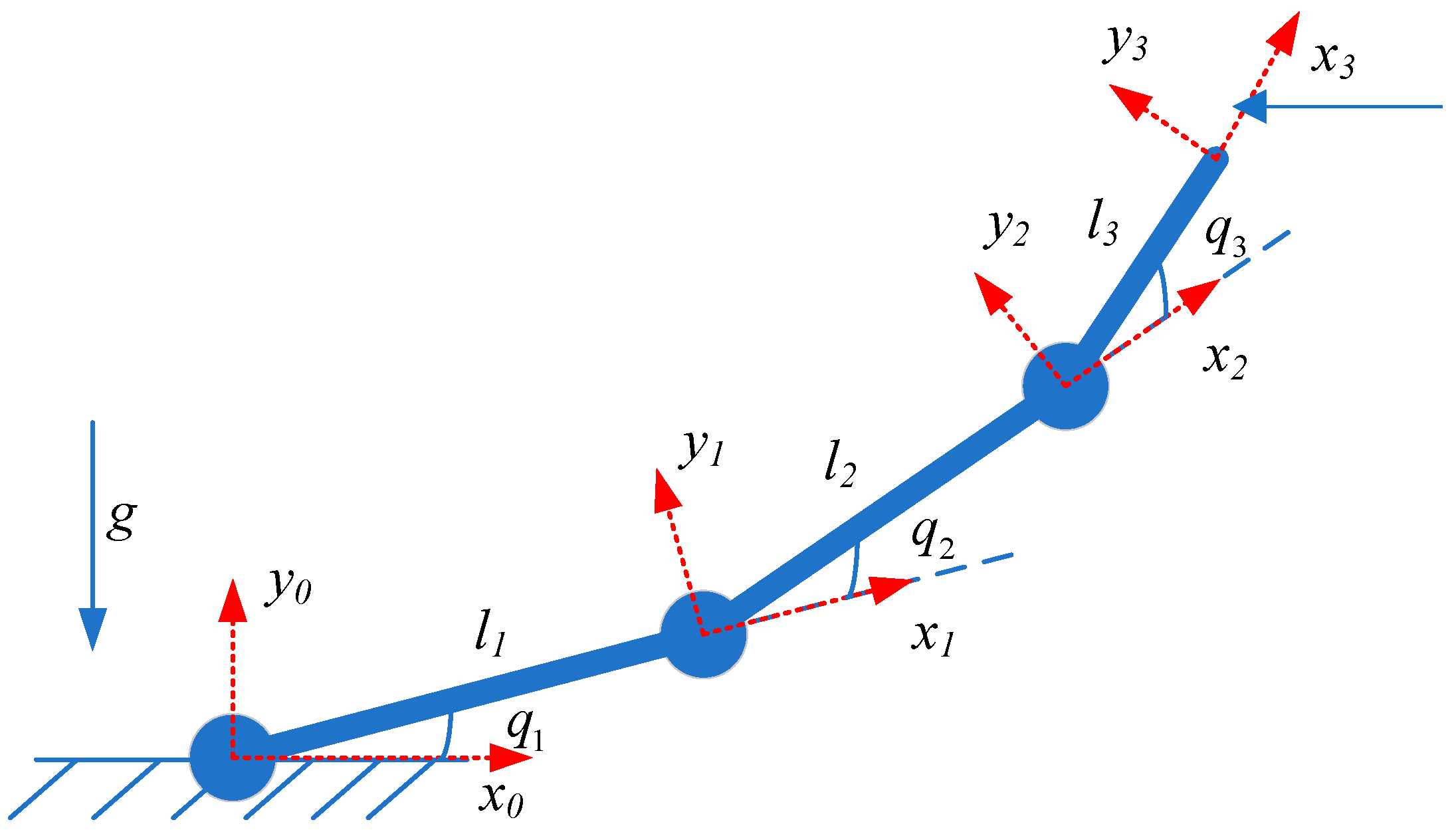
2. Robotic Manipulator Dynamics

In this paper, we consider an n-DOF manipulator under the presence of unknown friction, input dead-zone, and external disturbance. Its dynamics in the joint space are expressed by [2]

$$M(q)\ddot{q}+C(q,\dot{q})\dot{q}+G(q)+J^T\left(q\right)f_{ext}+{\mathsf{\tau }}_{fric}=H\left(\mathsf{\tau }\right),$$

(1)

where $q,\dot{q},\ddot{q}\in R^{n\times 1}$ present angular position, velocity, and acceleration vectors in the joint space of the manipulator, respectively; $M(q)\in R^{n\times n}$ presents the inertia matrix; $C(q,\dot{q})\in R^{n\times n}$ expresses the Coriolis and centrifugal term matrix; $G(q)\in R^{n\times 1}$ derives the gravity vector; $J\left(q\right)$ is a nonsingular Jacobian matrix; $f_{ext}$ presents the external disturbance vector; ${\mathsf{\tau }}_{fric}$ is the unknown friction vector; and $H\left(\mathsf{\tau }\right)$ is the torque vector acting on joints within the dead-zone.

The friction model, ${\mathsf{\tau }}_{fric}$, is exhibited as

$${\mathsf{\tau }}_{fric}=b\dot{q}+ctanh\left(\frac{\dot{q}}{\psi }\right),$$

(2)

where $b\in R^{n\times n}$ and $c\in R^{n\times n}$ are positive diagonal matrices; $\psi$ is a positive constant; and $tanh\left(\frac{\dot{q}}{\psi }\right)={\left[\tanh \left(\frac{{\dot{q}}_1}{\psi }\right),\dots ,\tanh \left(\frac{{\dot{q}}_n}{\psi }\right)\right]}^T\in R^{n\times 1}$.

Property 1 

[34].$M\left(q\right)$is a positive definite symmetric matrix and the condition$0<{\lambda }_{\min }\left(M\left(q\right)\right)\le \Vert M\left(q\right)\Vert \le {\lambda }_{\max }\left(M\left(q\right)\right)\le {\sigma }_0$holds where${\sigma }_0$is a positive constant, and${\lambda }_{\min }\left(M\right)$and${\lambda }_{\max }\left(M\right)$are the minimum and maximum eigenvalues of a matrix$M$.

Property 2 

[2].$\dot{M}\left(q\right)-2C\left(q,\dot{q}\right)$is a skew-symmetric matrix, that is provided as$x^T\left[\dot{M}\left(q\right)-2C\left(q,\dot{q}\right)\right]x=0$.

Assumption 1

[13].The input dead-zone nonlinearity presented in Figure 1 can be derived as follows:

$$H\left(\tau \right)=\{\begin{array}{cc}{h}_r\left(\tau -{\tau }_r\right)& \tau \ge {\tau }_r\\ 0& {\tau }_l<\tau <{\tau }_r\\ h_l\left(\tau -{\tau }_l\right)& \tau \le {\tau }_l\end{array},$$

(3)

where${\tau }_r$and${\tau }_l$are unknown constants for which:${\tau }_r>0$, ${\tau }_l<0$, and$H\left(\tau \right)={[H\left({\tau }_1\right),\dots ,H\left({\tau }_n\right)]}^T$.

Assumption 2.

The dead-zone nonlinear functions are smooth functions and their derivatives are bounded by unknown positive constants such that

$$\begin{array}{l}0<H_{r1}<{\dot{h}}_r\left(\tau -{\tau }_r\right)<H_{r2},\left[{\tau }_r,+\infty \right)\\ 0<H_{l1}<{\dot{h}}_l\left(\tau -{\tau }_l\right)<H_{l2},\left(-\infty ,{\tau }_l\right]\end{array}.$$

(4)

Based on Equations (3) and (4), the dead-zone functions can be represented as follows:

$$H\left(\tau \right)=\tau +\xi \left(t\right),$$

(5)

where $\xi \left(t\right)$ is an unknown vector whose elements are smooth functions. Additionally, their derivatives are bounded.

Let $x_1=q\in R^n$ and $x_2\in \dot{q}\in R^n$; then the robotic dynamics (1) can be rewritten as follows:

$$\begin{array}{c}{\dot{x}}_1=x_2\hfill \\ {\dot{x}}_2=M^{-1}\left(x_1\right)(u-C\left(x_1,x_2\right)x_2-G(x_1)-\Delta )\hfill \end{array},$$

(6)

where $x_i={[x_{i1},x_{i2},\dots ,x_{in}]}^T,(i=1,2)$; $\Delta =J^T(q)f_{ext}+{\mathsf{\tau }}_{fric}+\xi (t)$ derives a lumped disturbance including the unknown friction, external disturbance, and an unknown vector of the input dead-zone, and $u$ depicts the torque control signal.

In this paper, we design an advanced control to guarantee that the output responses track a reference $x_d={[x_{d1},x_{d2},\dots ,x_{dn}]}^T$ and satisfy the condition, ${\underset{\_}{k}}_{ci}(t)<x_{1i}(t)<{\overline{k}}_{ci}(t)$, where ${\underset{\_}{\mathbf{k}}}_c(t)={[{\underset{\_}{k}}_{c1}(t),\dots ,{\underset{\_}{k}}_{cn}(t)]}^T$ and ${\overline{k}}_c(t)={[{\overline{k}}_{c1}(t),\dots ,{\overline{k}}_{cn}(t)]}^T$ are time-varying functions.

Assumption 3.

In this study, we suppose that the manipulator operates in a bounded workspace. It means that the reference signals,$x_{di},i=1,2,\dots ,n$, are bounded and known, $|x_{di}|\le {\overline{X}}_{d0}$, and${\overline{X}}_{d0}$is a positive constant.

3. Control Design

Before we design the LESO to estimate the lumped disturbance and the unmeasured states in the manipulator, an extra state $x_3\in R^{n\times 1}$ is added in the manipulator dynamics (6) to present the lumped disturbance, $M^{-1}(x_1)\Delta$. The system state is presented as $x={[x_1^T,x_2^T,x_3^T]}^T\in R^{3n\times 1}$. Note that the extra state $x_3$ is continuously differentiable and bounded as in [35,36].

Assumption 4.

The difference of the state$x_3(t)$is assumed to be bounded, i.e.,${\Vert \mathsf{\delta }\left(t\right)\Vert }_{\infty }\le \overline{\delta }$, where$\overline{\delta }$is a positive constant.

The manipulator dynamics (6) is represented as follows:

$$\begin{array}{l}{\dot{x}}_1=x_2\\ {\dot{x}}_2=F\left(x_1,x_2\right)+H\left(x_1\right)u+x_3\\ {\dot{x}}_3=\mathsf{\delta }\left(t\right)\end{array},$$

(7)

where $\mathsf{\delta }(t)$ presents the derivative of the state $x_3(t)$; $x_3$ defines $-M^{-1}(x_1)\Delta$; $H(x_1)$ derives $M^{-1}(x_1)$; and $F(x_1,x_2)$ describes $-M^{-1}(x_1)(C(x_1,x_2)x_2+G(x_1))$.

Assumption 5.

We suppose that the functions$F(x_1,x_2)$are locally Lipschitz for$x_2$in its practical range.

3.1. Linear Extended State Observer Design

The LESO is designed to not only approximate the lumped disturbance, $x_3$, but also estimate the unmeasured system state vector, $x_2$. Let $\widehat{x}$ express the estimated system state of $x$ and let $\tilde{x}$ present the estimation error, $(\tilde{x}=x-\widehat{x})$. Now, we represent the robotic dynamics (7) as follows:

$$\begin{array}{l}\dot{x}=A_{n}x+B_{n}u+\varphi \left(x\right)+D\left(x\right)\\ y=x_1\end{array},$$

(8)

where $A_n=\left[\begin{array}{lll}{0}_{n\times n}\hfill & I_{n\times n}\hfill & 0_{n\times n}\hfill \\ 0_{n\times n}\hfill & 0_{n\times n}\hfill & I_{n\times n}\hfill \\ 0_{n\times n}\hfill & 0_{n\times n}\hfill & 0_{n\times n}\hfill \end{array}\right]\in R^{3n\times 3n}$; $B_n=\left[\begin{array}{l}{0}_{n\times n}\\ H\left(x_1\right)\\ 0_{n\times n}\end{array}\right]\in R^{3n\times n}$; $\varphi \left(x\right)=\left[\begin{array}{l}{0}_{n\times 1}\\ F\left(x\right)\\ 0_{n\times 1}\end{array}\right]\in R^{3n\times 1}$; and $D\left(x\right)=\left[\begin{array}{l}{0}_{n\times 1}\\ 0_{n\times 1}\\ \mathsf{\delta }\end{array}\right]\in R^{3n\times 1}$.

The extended state observer is presented as follows:

$$\dot{\widehat{x}}=A_n\widehat{x}+B_{n}u+\varphi \left(\widehat{x}\right)+\mathsf{\kappa }\left(x_1-{\widehat{x}}_1\right),$$

(9)

where $\varphi (\widehat{x})={[\begin{array}{lll}{0}_{n\times n}\hfill & F\left(x_1,{\widehat{x}}_2\right)\hfill & 0_{n\times n}\hfill \end{array}]}^T$, $\mathsf{\kappa }={[\begin{array}{lll}3{\kappa }_0{I}_{n\times n}\hfill & 3{\kappa }_0^2{I}_{n\times n}\hfill & {\kappa }_0^3{I}_{n\times n}\hfill \end{array}]}^T\in R^{3n\times n}$ presents the observer gain matrix; and ${\kappa }_0>0$ is adjusted to enhance the observer performance.

From Equations (8) and (9), the estimation error dynamics is computed as

$$\dot{\tilde{x}}=A_n\tilde{x}+\varphi \left(x\right)-\varphi \left(\widehat{x}\right)-\mathsf{\kappa }{\tilde{x}}_1+D\left(x\right),$$

(10)

where $D\left(x\right)={[\begin{array}{ccc}{0}_{n\times n}& 0_{n\times n}& \mathsf{\delta }\left(t\right)\end{array}]}^T$. Now, we define ${\zeta }_i=\frac{{\tilde{x}}_i}{{\kappa }_0{}^{i-1}}\in R^{n\times 1}\left(i=1,2,3\right)$, $\tilde{\varphi }\stackrel{\Delta }{=}\varphi \left(x\right)-\varphi \left(\widehat{x}\right)$, and then the LESO (10) is represented as

$$\dot{\zeta }={\kappa }_0{A}_{n1}\zeta +\frac{\tilde{\varphi }}{{\kappa }_0}+\frac{D\left(x\right)}{{\kappa }_0^2},$$

(11)

where $A_{n1}=\left[\begin{array}{lll}-3I_{n\times n}\hfill & I_{n\times n}\hfill & 0_{n\times n}\hfill \\ -3I_{n\times n}\hfill & 0_{n\times n}\hfill & I_{n\times n}\hfill \\ -I_{n\times n}\hfill & 0_{n\times n}\hfill & 0_{n\times n}\hfill \end{array}\right]\in R^{3n\times 3n}$ is a Hurwitz matrix.

From Assumption 5, the below inequality can be obtained:

$$|\tilde{\varphi }|=|\varphi \left(x_2\right)-\varphi \left({\widehat{x}}_2\right)|\le c|{\zeta }_2|.$$

(12)

Theorem 1. 

When the LESO (9) is used to estimate the lumped disturbance of the unmeasured states, and the inequality (12) is guaranteed, then the estimation errors are bounded with the appropriate constant.

Proof of Theorem 1.

A Lyapunov function is taken into account as follows:

$$V_0=\frac{1}{2}{\zeta }^{T}P\zeta ,$$

(13)

where $P$ derives a positive definite matrix. It is chosen as a solution of the following Lyapunov equation:

$$A_{n1}^{T}P+P{A}_{n1}=-2I_{3n\times 3n}.$$

(14)

From (11), the differential Lyapunov function is presented as

$$\begin{array}{cc}{\dot{V}}_0& =\frac{1}{2}{\kappa }_0{\zeta }^T\left(A_{n1}^{T}P+P{A}_{n1}\right)\zeta +\frac{1}{2}{\left(\frac{\tilde{\varphi }}{{\kappa }_0}+\frac{D\left(x\right)}{{\kappa }_0^2}\right)}^{T}P\zeta +\frac{1}{2}{\zeta }^{T}P\left(\frac{\tilde{\varphi }}{{\kappa }_0}+\frac{D\left(x\right)}{{\kappa }_0^2}\right)\hfill \\ & =-{\kappa }_0{\zeta }^T\zeta +{\left(\frac{\tilde{\varphi }}{{\kappa }_0}+\frac{D\left(x\right)}{{\kappa }_0^2}\right)}^{T}P\zeta \le -\left({\kappa }_0-\frac{c}{{\kappa }_0}\right){\Vert \zeta \Vert }_2^2+\frac{\overline{\delta }}{{\kappa }_0^2}{\lambda }_{\max }\left(P\right){\Vert \zeta \Vert }_2\hfill \\ & =\left(-\left({\kappa }_0-\frac{c}{{\kappa }_0}\right){\Vert \zeta \Vert }_2+\frac{\overline{\delta }}{{\kappa }_0^2}{\lambda }_{\max }\left(P\right)\right){\Vert \zeta \Vert }_2\hfill \end{array}.$$

(15)

The differential Lyapunov Function (15) is negative when $-\left({\kappa }_0-\frac{c}{{\kappa }_0}\right){\Vert \zeta \Vert }_2+\frac{\overline{\delta }}{{\kappa }_0^2}{\lambda }_{\max }\left(P\right)\le 0$; that implies ${\Vert \zeta \Vert }_2\ge \frac{\overline{\delta }}{{\kappa }_0\left({\kappa }_0^2-c\right)}{\lambda }_{\max }\left(P\right)$. The estimation errors in LESO are reducing and the stability of the ESO is guaranteed [37] when the bandwidth, ${\kappa }_0$, increases. □

3.2. Proposed Control Design

Figure 2 presents the structure of the proposed control with an n-DOF manipulator under the presence of unknown external disturbance, friction, input dead-zone, and output constraints. The proposed control consists of a full state feedback control based on the BLF, and a linear extended state observer. The backstepping control is designed with the barrier Lyapunov function to avoid the violation of the output constraint. Because all states, such as position and velocity, of the manipulator are used to design the backstepping control, this control is named as a full state feedback control-based barrier Lyapunov function. The extended state observer was employed to approximate the lumped disturbance in the manipulator dynamics and unmeasured variable, ${\widehat{x}}_2$.

The tracking errors, $e_i,\left(i=1,2\right)$, are defined as

$$\begin{array}{l}{e}_1=x_1-x_d\in R^{n\times 1}\\ e_2=x_2-{\mathsf{\alpha }}_1\in R^{n\times 1}\end{array},$$

(16)

where $x_d\in R^{n\times 1}$ is the reference signal.

The time-varying upper and lower boundary errors of $e_1$ are computed as:

$$\begin{array}{l}{k}_{ai}\left(t\right)={\overline{k}}_{ci}\left(t\right)-x_{di}\left(t\right)\\ k_{bi}\left(t\right)={\underset{\_}{k}}_{ci}\left(t\right)-x_{di}\left(t\right)\end{array},$$

(17)

where ${\underset{\_}{k}}_{ci}(t)\le x_{1i}(t)\le {\overline{k}}_{ci}(t)$, $k_{ai}$ is the time-varying upper boundary error, and $k_{bi}$ is the time-varying lower boundary error.

The virtual control, ${\mathsf{\alpha }}_1$ is computed as

$${\mathsf{\alpha }}_1=-K_1{e}_1-{\lambda }_1{e}_1+{\dot{x}}_d,$$

(18)

where ${\lambda }_1\in R^{n\times n}$ is a positive diagonal matrix; ${\lambda }_1=diag\left(\left[{\lambda }_{11},\dots ,{\lambda }_{1n}\right]\right)\in R^{n\times n}$ expresses a positive diagonal matrix. The elements in the matrix ${\lambda }_1$ are stated as

$${\lambda }_{1i}=\sqrt{{\left(\frac{{\dot{k}}_{ai}\left(t\right)}{k_{ai}\left(t\right)}\right)}^2+{\left(\frac{{\dot{k}}_{bi}\left(t\right)}{k_{bi}\left(t\right)}\right)}^2}.$$

(19)

The control input is calculated as follows:

$$u=-{\mathsf{\kappa }}_{\xi }-K_2{e}_2-M\left(x_1\right){\widehat{x}}_3+C\left(x_1,{\widehat{x}}_2\right){\mathsf{\alpha }}_1+G\left(x_1\right)+M\left(x_1\right){\dot{\mathsf{\alpha }}}_1,$$

(20)

where ${\mathsf{\kappa }}_{\xi }=\left[\left(\frac{h\left(e_{11}\right)}{k_{a1}^2-e_{11}^2}+\frac{1-h\left(e_{11}\right)}{k_{b1}^2-e_{11}^2}\right)e_{11},\dots ,\left(\frac{h\left(e_{1n}\right)}{k_{an}^2-e_{1n}^2}+\frac{1-h\left(e_{1n}\right)}{k_{bn}^2-e_{1n}^2}\right)e_{1n}\right]\in R^{n\times 1}$, $h\left(e_{1i}\right)$ is derived as follows

$$h\left(e_{1i}\right)=\{\begin{array}{l}0, e_{1i}\le 0\\ 1, otherwise\end{array},i=1,\dots ,n,$$

(21)

and $K_2\in R^{n\times n}$ is a positive diagonal matrix.

3.3. Stability Analysis

Lemma 1 

[22].The following inequality holds for any positive constant$k\in \mathrm{R}$and$x\in \mathrm{R}$so that$|x|<k$:

$$\log \frac{k^2}{k^2-x^2}\le \frac{x^2}{k^2-x^2}.$$

(22)

Theorem 2.

The control law in (18) and (20), which utilizes the estimation value of the unmeasurable state, and the lumped disturbance from the ESO in (9) guarantee the ultimately uniformly bounded tracking performance and satisfaction of the output constraint in (17) of the manipulator described by (1), under unknown friction, external disturbance, and an unknown vector of the input dead-zone.

Proof of Theorem 2.

Step 1. We take the time derivative of the position error $e_1$ shown as

$${\dot{e}}_1=x_2-{\dot{x}}_d=e_2+{\mathsf{\alpha }}_1-{\dot{x}}_d.$$

(23)

From (18), substituting the virtual control signal, ${\mathsf{\alpha }}_1$, into (23), the result is represented as

$${\dot{e}}_1=e_2-K_1{e}_1-{\lambda }_1{e}_1.$$

(24)

Based on Yu et al. [38], to guarantee the constrained performance of the joint angles, we can select a barrier Lyapunov function as follows:

$$V_1=\frac{1}{2}{\displaystyle \sum _{i=1}^n\left(h\left(e_{1i}\right)\log \left(\frac{k_{ai}^2}{k_{ai}^2-e_{1i}^2}\right)+\left(1-h\left(e_{1i}\right)\right)\log \left(\frac{k_{bi}^2}{k_{bi}^2-e_{1i}^2}\right)\right)}.$$

(25)

In order to simplify the BLF (25), we state variables by

$${\xi }_{ai}=\frac{e_{1i}}{k_{ai}},{\xi }_{bi}=\frac{e_{1i}}{k_{bi}},{\xi }_i=h\left(e_{1i}\right){\xi }_{ai}+\left(1-h\left(e_{1i}\right){\xi }_{bi}\right).$$

(26)

As a result, the Lyapunov Function (25) is rewritten as follows:

$$V_1={\displaystyle \sum _{i=1}^n\frac{1}{2}\log \frac{1}{1-{\xi }_i^2}}.$$

(27)

The differential barrier Lyapunov function is calculated by

$${\dot{V}}_1={\displaystyle \sum _{i=1}^n\left(\frac{h\left(e_{1i}\right){\xi }_{ai}}{\left(1-{\xi }_{ai}^2\right)k_{ai}}\left({\dot{e}}_{1i}+\frac{{\dot{k}}_{a1}}{k_{ai}}{e}_{1i}\right)+\frac{\left(1-h\left(e_{1i}\right)\right){\xi }_{bi}}{\left(1-{\xi }_{bi}^2\right)k_{bi}}\left({\dot{e}}_{1i}+\frac{{\dot{k}}_{b1}}{k_{bi}}{e}_{1i}\right)\right)}.$$

(28)

Substituting (24) into (28), the result presents as

$$\begin{array}{cc}{\dot{V}}_1& ={\displaystyle \sum _{i=1}^n\left(\frac{h\left(e_{1i}\right){\xi }_{ai}}{\left(1-{\xi }_{ai}^2\right)k_{ai}}\left(e_{2i}-\left(k_{ai}+{\overline{k}}_{1i}+\frac{{\dot{k}}_{a1}}{k_{ai}}\right)e_{1i}\right)+\frac{\left(1-h\left(e_{1i}\right)\right){\xi }_{bi}}{\left(1-{\xi }_{bi}^2\right)k_{bi}}\left({\dot{e}}_{1i}-\left(k_{bi}+{\overline{k}}_{1i}+\frac{{\dot{k}}_{b1}}{k_{bi}}\right)e_{1i}\right)\right)}\hfill \\ & \le -{\displaystyle \sum _{i=1}^n{k}_{1i}\frac{{\xi }^2}{1-{\xi }^2}}+{\mathsf{\kappa }}_{\xi }{e}_2\hfill \end{array}.$$

(29)

Step 2. Based on (6), the time derivative of error, $e_2$ is expressed as follows

$${\dot{e}}_2={\dot{x}}_2-{\dot{\mathsf{\alpha }}}_1=M{\left(x_1\right)}^{-1}\left[u-C\left(x_1,x_2\right)x_2-G\left(x_1\right)-\Delta \left(t\right)\right]-{\dot{\mathsf{\alpha }}}_1.$$

(30)

From (30) and (20), the time derivative of error, ${\dot{e}}_2$ is represented as

$$\begin{array}{cc}{\dot{e}}_2& =M{\left(x_1\right)}^{-1}[-C\left(x_1,x_2\right)x_2-G\left(x_1\right)-\Delta \left(t\right)\hfill \\ & -{\mathsf{\kappa }}_{\xi }-K_2{\widehat{e}}_2-M\left(x_1\right){\widehat{x}}_3+C\left(x_1,{\widehat{x}}_2\right){\mathsf{\alpha }}_1+G\left(x_1\right)+M\left(x_1\right){\dot{\mathsf{\alpha }}}_1]-{\dot{\mathsf{\alpha }}}_1\hfill \\ & =M{\left(x_1\right)}^{-1}\left[-{\mathsf{\kappa }}_{\xi }-K_2\left(e_2-{\tilde{x}}_2\right)-\Delta \left(t\right)-M\left(x_1\right){\widehat{x}}_3-C\left(x_1,x_2\right)e_2+\Delta C\left(x_1,{\tilde{x}}_2\right){\mathsf{\alpha }}_1\right]\hfill \end{array}.$$

(31)

To consider the stability of the dynamics system (1), including not only the position tracking performance at Step 1, but also the speed tracking performance (31), the following Lyapunov function is investigated as

$$V_2=V_1+\frac{1}{2}{e}_2^{T}M\left(x_1\right)e_2.$$

(32)

Next, the time derivative of the Lyapunov function (32) is calculated as

$${\dot{V}}_2={\dot{V}}_1+e_2^{T}M\left(x_1\right){\dot{e}}_2+\frac{1}{2}{e}_2^T\dot{M}\left(x_1\right)e_2.$$

(33)

Replacing (29) and (31) into (33) with property 2, the result is expressed by

$$\begin{array}{cc}{\dot{V}}_2=& -{\displaystyle \sum _{i=1}^n{k}_{1i}\frac{{\xi }^2}{1-{\xi }^2}}-e_2^T{K}_2{e}_2+e_2^T{c}_0|{\zeta }_2|-e_2^T\left(\Delta \left(t\right)+M\left(x_1\right){\widehat{x}}_3\right)\hfill \\ & +e_2^T{K}_2{\tilde{x}}_2+\Delta C\left(x_1,{\tilde{x}}_2\right){\mathsf{\alpha }}_1\hfill \end{array}.$$

(34)

In order to demonstrate the stability of the entire closed-loop system, including the estimation performance of the ESO, we choose a Lyapunov function via (15) and (32) as follows:

$$V=V_0+V_2=\frac{1}{2}{\zeta }^{T}P\zeta +\frac{1}{2}{\displaystyle \sum _{i=1}^n\log \frac{1}{1-{\xi }_i^2}}+\frac{1}{2}{e}_2^{T}M\left(x_1\right)e_2.$$

(35)

The time derivative of the Lyapunov Function (35) is computed as

$$\begin{array}{cc}\dot{V}& =-{\displaystyle \sum _{i=1}^n{k}_{1i}\frac{{\xi }^2}{1-{\xi }^2}}-\left({\kappa }_0-\frac{c}{{\kappa }_0}\right){\Vert \zeta \Vert }_2^2+\frac{\overline{\delta }}{{\kappa }_0^2}{\lambda }_{\max }\left(P\right){\Vert \zeta \Vert }_2-e_2^T{K}_2{e}_2\hfill \\ & -e_2^T\left(\Delta \left(t\right)-M\left(x_1\right){\widehat{x}}_3\right)+e_2^T{K}_2{\tilde{x}}_2+\Delta C\left(x_1,{\tilde{x}}_2\right){\mathsf{\alpha }}_1\hfill \end{array}.$$

(36)

We define $\epsilon \stackrel{\Delta }{=}\Delta \left(t\right)-M\left(x_1\right){\widehat{x}}_3\in R^{n\times 1}$ as the disturbance estimation error. These inequalities hold: $-e_2^T\mathsf{\epsilon }\le \frac{1}{2}{e}_2^T{e}_2+\frac{1}{2}{\mathsf{\epsilon }}^T\mathsf{\epsilon }$ and $e_2^T{K}_2{\tilde{x}}_2\le \frac{1}{2}{e}_2^T{K}_2{e}_2+\frac{1}{2}{\tilde{x}}_2^T{K}_2{\tilde{x}}_2$. Thus, when Lemma 1 is investigated, Equation (36) is rewritten as below:

$$\begin{array}{l}\dot{V}\le -\left({\kappa }_0-\frac{c}{{\kappa }_0}\right){\Vert \zeta \Vert }_2^2-K_1{\displaystyle \sum _{i=1}^n\log \frac{1}{1-{\xi }_i^2}}-\frac{1}{2}{e}_2^T\left(K_2-I_{n\times n}\right)e_2\\ +\frac{1}{2}{\mathsf{\epsilon }}^T\mathsf{\epsilon }+\frac{\overline{\delta }}{{\kappa }_0^2}{\lambda }_{\max }\left(P\right){\Vert \zeta \Vert }_2+\frac{1}{2}{\tilde{x}}_2^T{K}_2{\tilde{x}}_2+\Delta C\left(x_1,{\tilde{x}}_2\right){\mathsf{\alpha }}_1\le -c_{o}V+D_2\end{array},$$

(37)

where $c_0=\min \left({\lambda }_{\min }\left(\left({\kappa }_0-\frac{c}{{\kappa }_0}\right)P^{-1}\right),2{\lambda }_{\min }\left(K_1\right),{\lambda }_{\min }\left(\left(K_2-I\right)M^{-1}\right)\right)$ and $D=\Vert \frac{1}{2}{\mathsf{\epsilon }}^T\mathsf{\epsilon }+\frac{\overline{\delta }}{{\kappa }_0^2}{\lambda }_{\max }\left(P\right){\Vert \zeta \Vert }_2$ ${+\frac{1}{2}{\tilde{x}}_2^T{K}_2{\tilde{x}}_2+\Delta C\left(x_1,{\tilde{x}}_2\right){\mathsf{\alpha }}_1\Vert }_{\infty }$.

From Reference [39], we can state that when the system is controlled by the proposed control, it is ultimately uniformly bounded under the presence of unknown frictions, external disturbances, and input dead-zone. From (37), we can find the inequation as follows:

$$0\le V\left(t\right)\le \mu +\left(V\left(0\right)-\mu \right)e^{-c_{0}t}\le \mu +V\left(0\right),$$

(38)

where $\mu =\frac{D_2}{c_0}$.

From (25), (26), (35) and (38), we achieve the results as

$$\frac{1}{2}\log \frac{1}{1-{\xi }_i^2}\le \mu +V\left(0\right),$$

(39)

$$\{\begin{array}{cc}\frac{1}{2}\log \left(\frac{k_{ai}^2}{k_{ai}^2-e_{1i}^2}\right)\le \mu +V\left(0\right)& ,e_{1i}>0\\ \frac{1}{2}\log \left(\frac{k_{bi}^2}{k_{bi}^2-e_{1i}^2}\right)\le \mu +V\left(0\right)& ,e_{1i}\le 0\end{array}.$$

(40)

After we take the exponentials on both sides of (40), the results are given as

$$\{\begin{array}{cc}\frac{k_{ai}^2}{k_{ai}^2-e_{1i}^2}\le e^{2\left(\mu +V\left(0\right)\right)}& ,e_{1i}>0\\ \frac{k_{bi}^2}{k_{bi}^2-e_{1i}^2}\le e^{2\left(\mu +V\left(0\right)\right)}& ,e_{1i}\le 0\end{array}.$$

(41)

The following inequality can then be achieved:

$$\{\begin{array}{cc}{e}_{1i}\le k_{ai}\sqrt{1-e^{-2\left(\mu +V\left(0\right)\right)}}& ,e_{1i}>0\\ e_{1i}\ge -k_{bi}\sqrt{1-e^{-2\left(\mu +V\left(0\right)\right)}}& ,e_{1i}\le 0\end{array}.$$

(42)

As a result, we can conclude that the output constraints are guaranteed. The proof is complete. □

4. Numerical Simulations

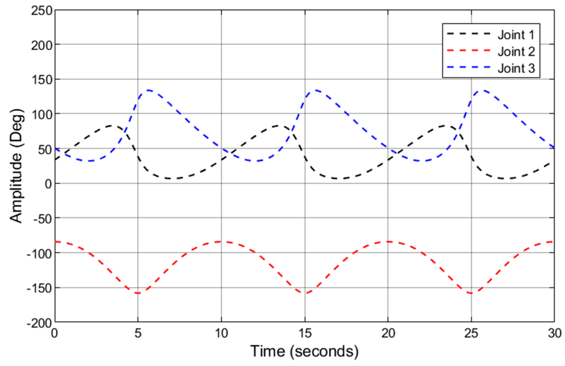
4.1. Simulation Descriptions

Some simulations were conducted on MATLAB Simulink with a 3-DOF planar manipulator to illustrate the superiorities of the proposed control. The MATLAB Simulink was configured with a sampling time of 0.001 s; the solver type was ODE3. Additionally, the simulation time was 30 s.

The 3-DOF planar manipulator presented in Figure 3 is a planar robot with 3 rotary actuators. The parameters of the manipulator are presented in

Table 1. Parameters of the 3-DOF planar manipulator.

Symbol	Description	Symbol	Description
l1 = 0.35 m	Length of 1st link	m1 = 0.23 kg	Mass of 1st link
l2 = 0.3 m	Length of 2nd link	m2 = 0.2 kg	Mass of 2nd link
l3 = 0.15 m	Length of 3rd link	m3 = 0.1 kg	Mass of 3rd link
g = 9.81 ms−2	Gravity constant	-	-

. Additionally, all mass exists as a point mass at the distal end of each link, and the center of mass in each link is presented by ${}^i{P}_C=l_i{X}_i{,}_{\left(i=1,2,3\right)}$. By using the Newton iteration method in [2], the dynamics of the manipulator are presented in the Appendix A.

The friction model vector includes the viscous and coulomb frictions, which is presented as follows:

$${\mathsf{\tau }}_{fric}=b\dot{q}+c tanh\left(\frac{\dot{q}}{\psi }\right)\in R^3,$$

(43)

where $b=0.5diag([1,1,1])(\mathrm{Nms}/\mathrm{rad})$, $c=0.2diag([1,1,1])(\mathrm{Nm})$, and $\psi =10$. The dead-zone functions are defined as $h_r(\tau -{\tau }_r)=(\tau -{\tau }_r);h_r(\tau -{\tau }_l)=1.2(\tau -{\tau }_l)$, where ${\tau }_r=0.2$ and ${\tau }_l=-0.2$. During the simulation period, an external disturbance along the x-axis of the original coordinate system is applied after the 20th second, as $f=-40(\mathrm{N})$. The trajectory signals, $x_d$ and $z_d$, in the Cartesian coordinate, are sine waves, $x_d=0.4+0.2\cos (2\pi f_{fre}t)(\mathrm{m})$, $y_d=0(\mathrm{m})$, and $z_d=0.2\sin (2\pi f_{fre}t)(\mathrm{m})$, where $f_{fre}$ is the frequency of the trajectory. Additionally, the rotary angle around the z-axis is zero.

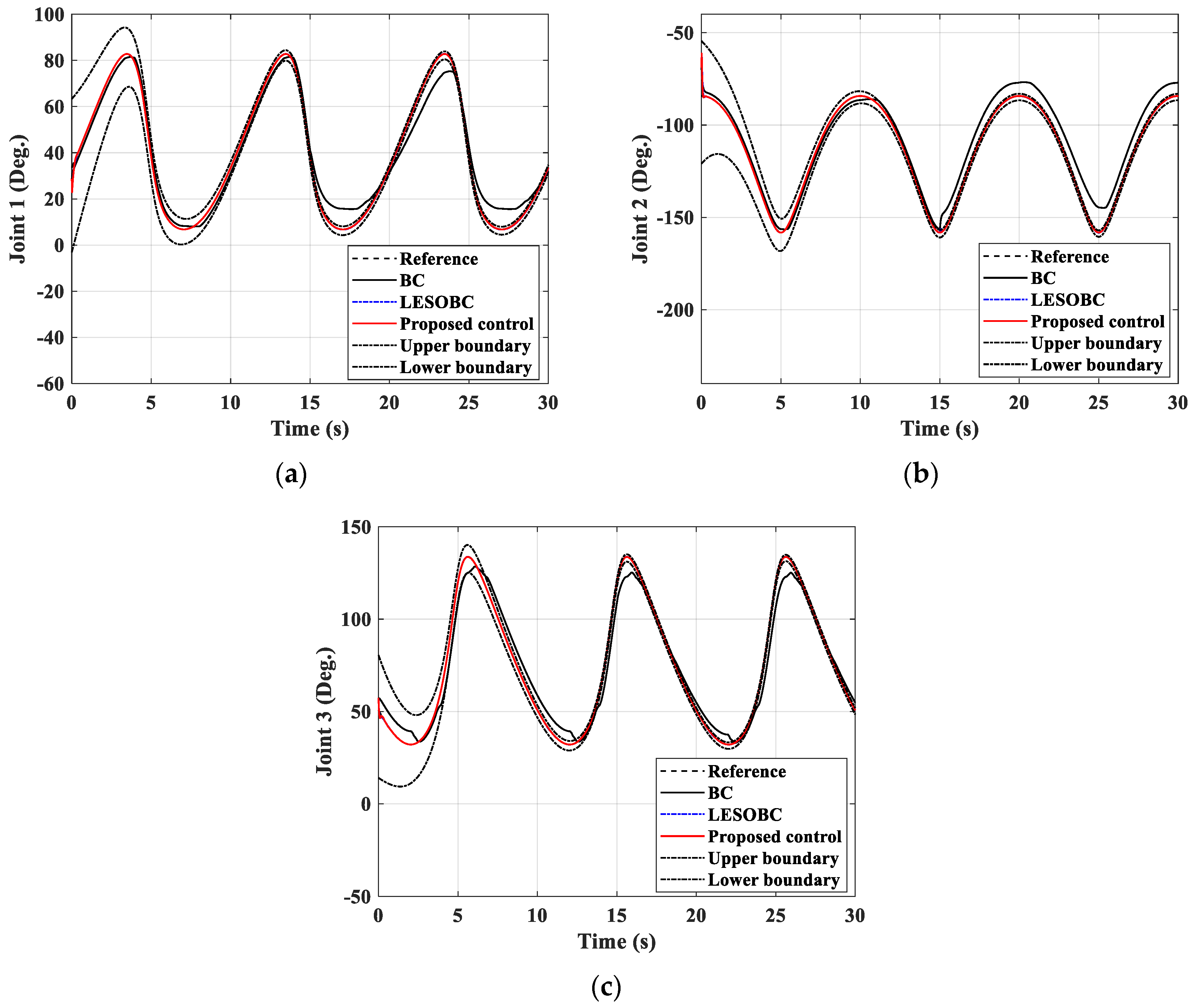
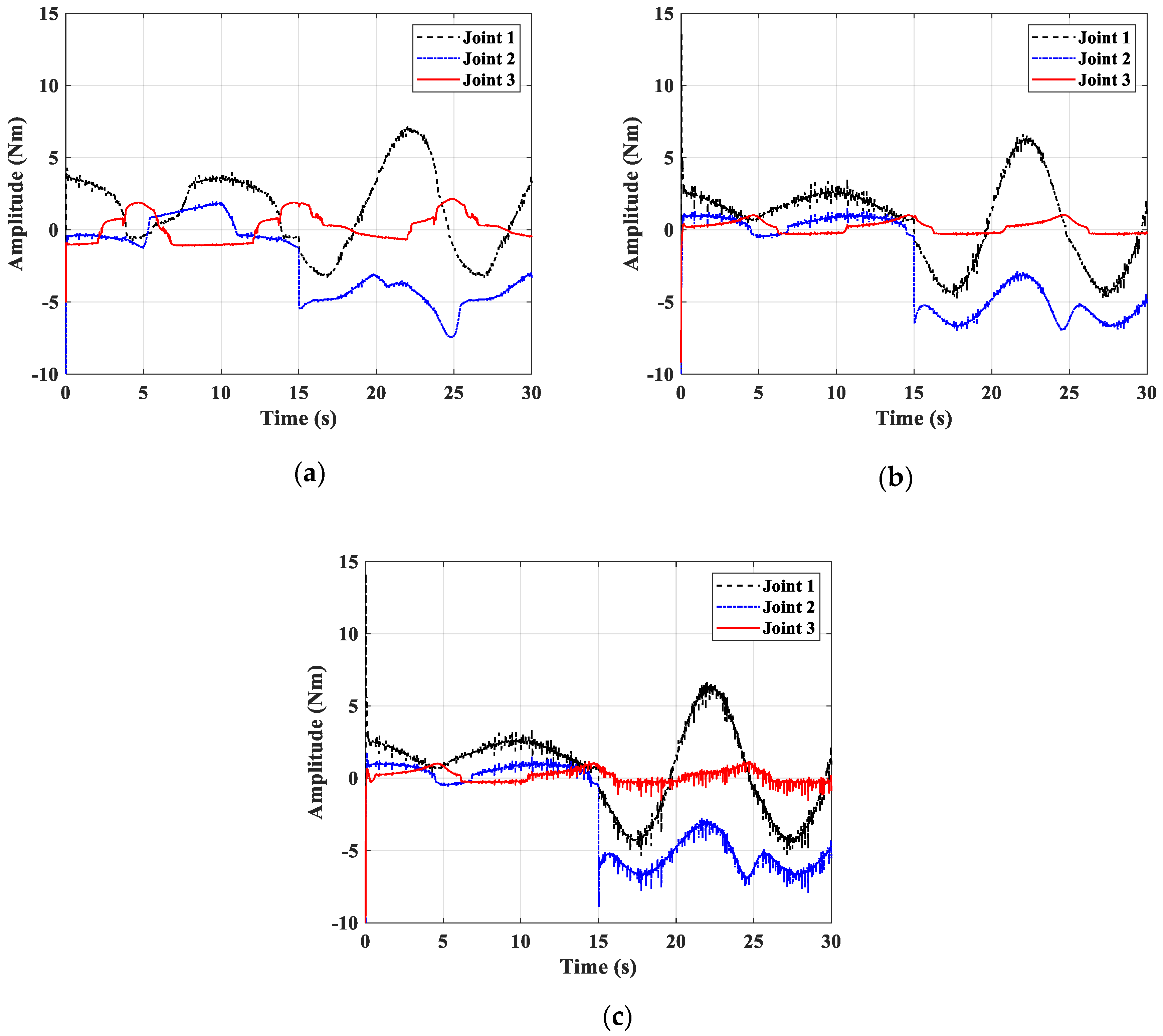
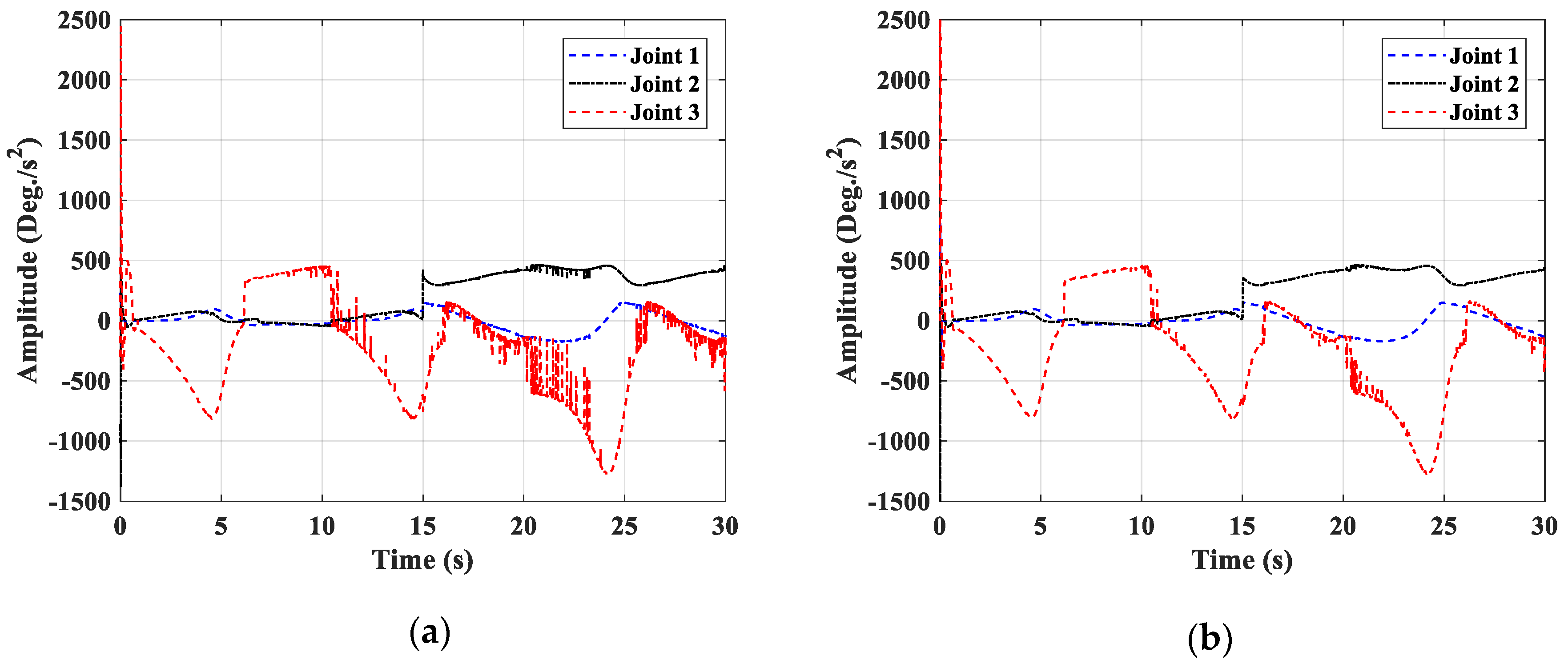
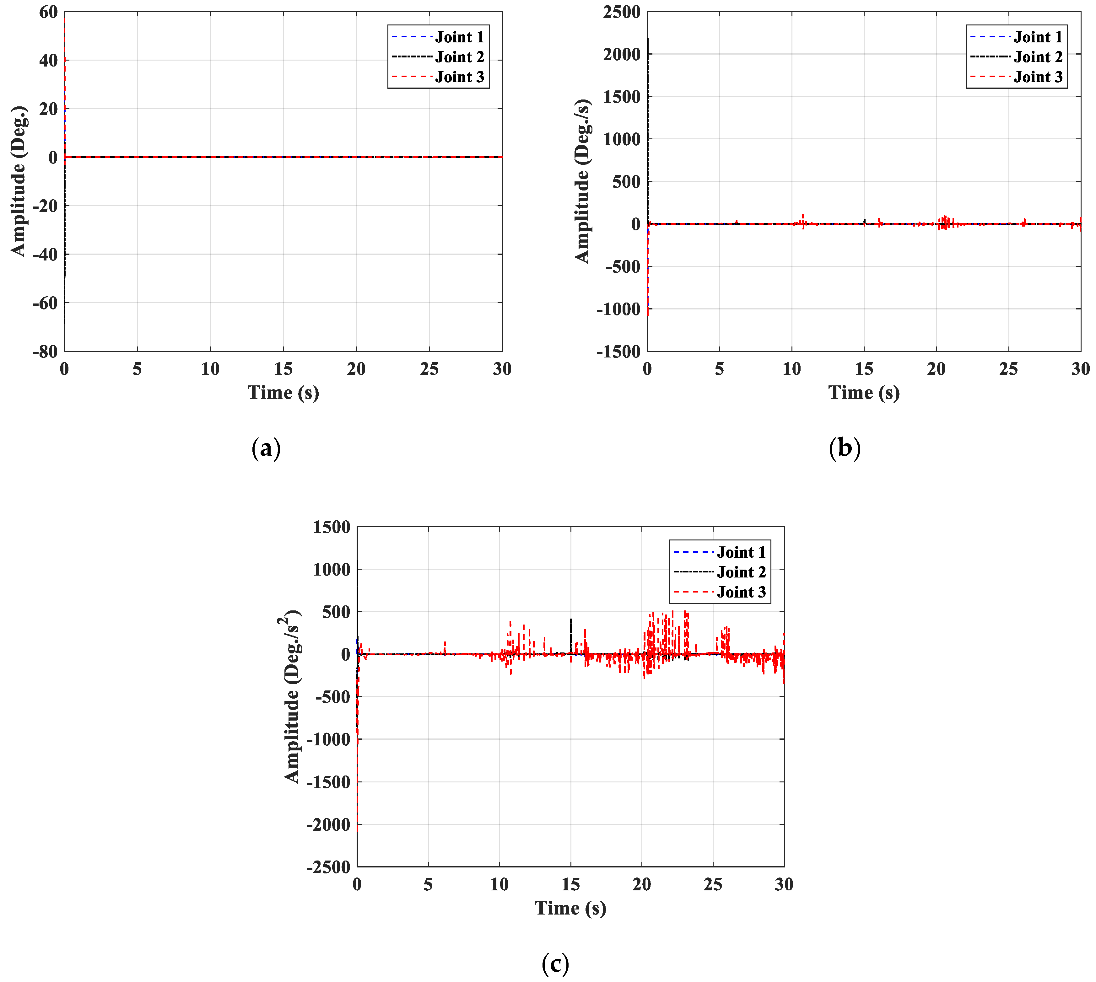
4.2. Simulation Results

The merits of the proposed controller are illustrated through comparisons with two other controllers:

• The backstepping control (BC):

  $$u=-K_2{e}_2+C\left(x_1,x_2\right){\mathsf{\alpha }}_1\left(t\right)+G\left(x_1\right)+M\left(x_1\right){\dot{\mathsf{\alpha }}}_1\left(t\right)-e_1$$

  (44)

  $${\mathsf{\alpha }}_1=x_{2d}-K_1{e}_1$$

  (45)
• The linear extended state observer via backstepping control (LESOBC):

  $$u=-K_2{e}_2+C\left(x_1,{\widehat{x}}_2\right){\mathsf{\alpha }}_1\left(t\right)+G\left(x_1\right)+M\left(x_1\right){\dot{\mathsf{\alpha }}}_1\left(t\right)-e_1-M\left(x_1\right){\widehat{x}}_3,$$

  (46)

  $${\mathsf{\alpha }}_1=x_{2d}-K_1{e}_1$$

  (47)

  where ${\widehat{x}}_3$ is the estimated lumped disturbance. This estimated lumped disturbance is approximated by the LESO in (9).

The parameters of these controllers are exhibited in

Table 2. Parameters of the three controllers.

Controllers	Parameters
Backstepping control	$K_1=10diag\left(\left[2,2,1.5\right]\right)$, $K_2=30diag\left(\left[1.5,1.5,0.5\right]\right)$;
LESOBC	$K_1=10diag\left(\left[2,2,1.5\right]\right)$, $K_2=30diag\left(\left[1.5,1.5,0.5\right]\right)$; ${\kappa }_0=200$
Proposed control	$K_1=10diag\left(\left[2,2,1.5\right]\right)$, $K_2=30diag\left(\left[1.5,1.5,0.5\right]\right)$; ${\kappa }_0=200$, $k_{a1}\left(t\right)=\left(0.5e^{-0.6t}+0.02\right){\left[\begin{array}{lll}1\hfill & 1\hfill & 1\hfill \end{array}\right]}^T$, $k_{b1}\left(t\right)=-\left(0.6e^{-0.6t}+0.04\right){\left[\begin{array}{lll}1\hfill & 1\hfill & 1\hfill \end{array}\right]}^T$

. In order to ensure equality in comparisons between the controllers, parameters of the backstepping are firstly selected. Next, some parameters of the LESOBC are inherited from the BC, and others, the observer gains, are adjusted. Finally, the proposed control copies the parameters in the LESOBC and uses the upper and lower boundaries.

The simulations are divided into two cases. In the first case, we conduct simulations with the low-frequency references which are set to 0.1 Hz. In the second case, the frequency of the reference is increased to 0.5 Hz.

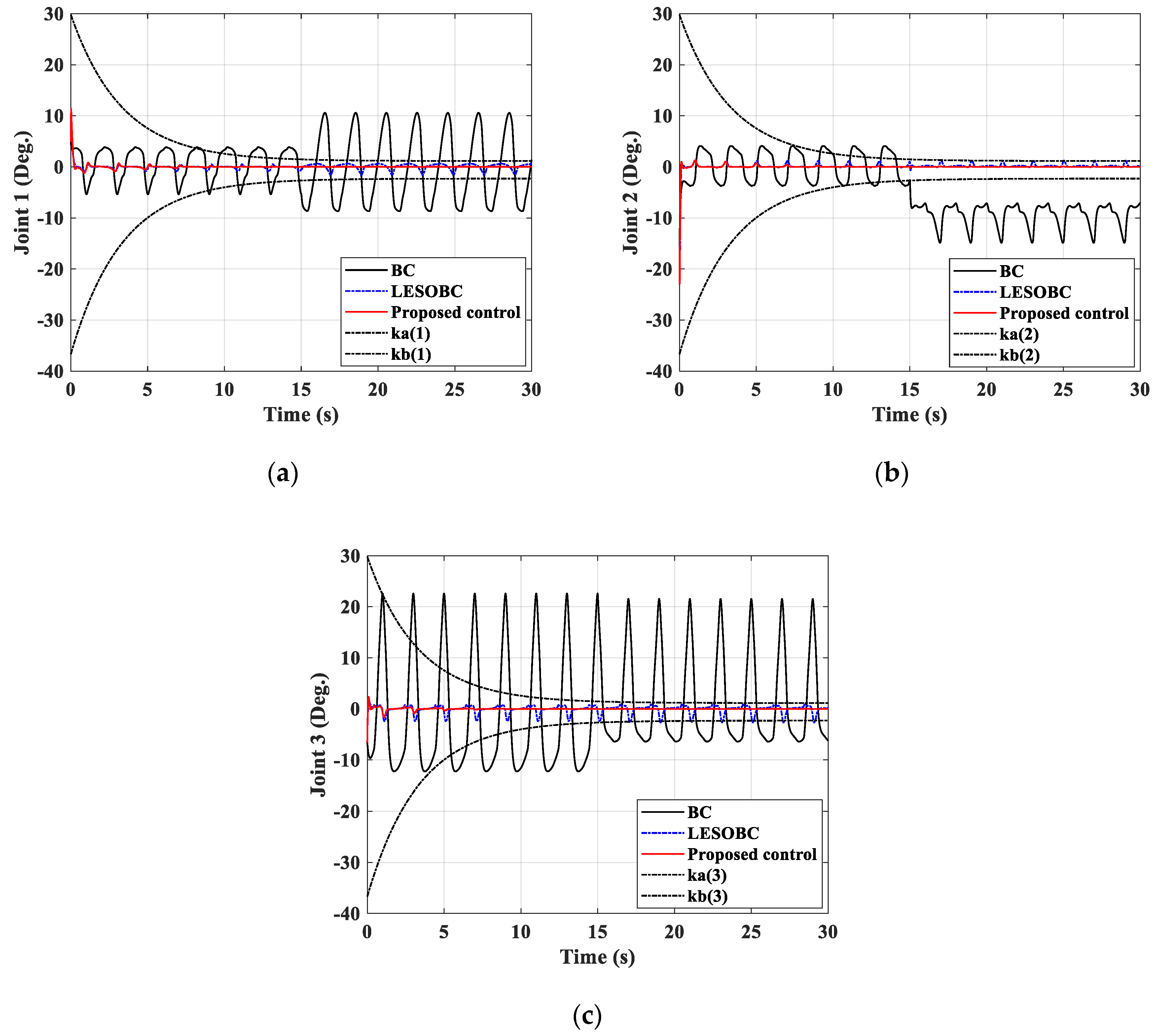
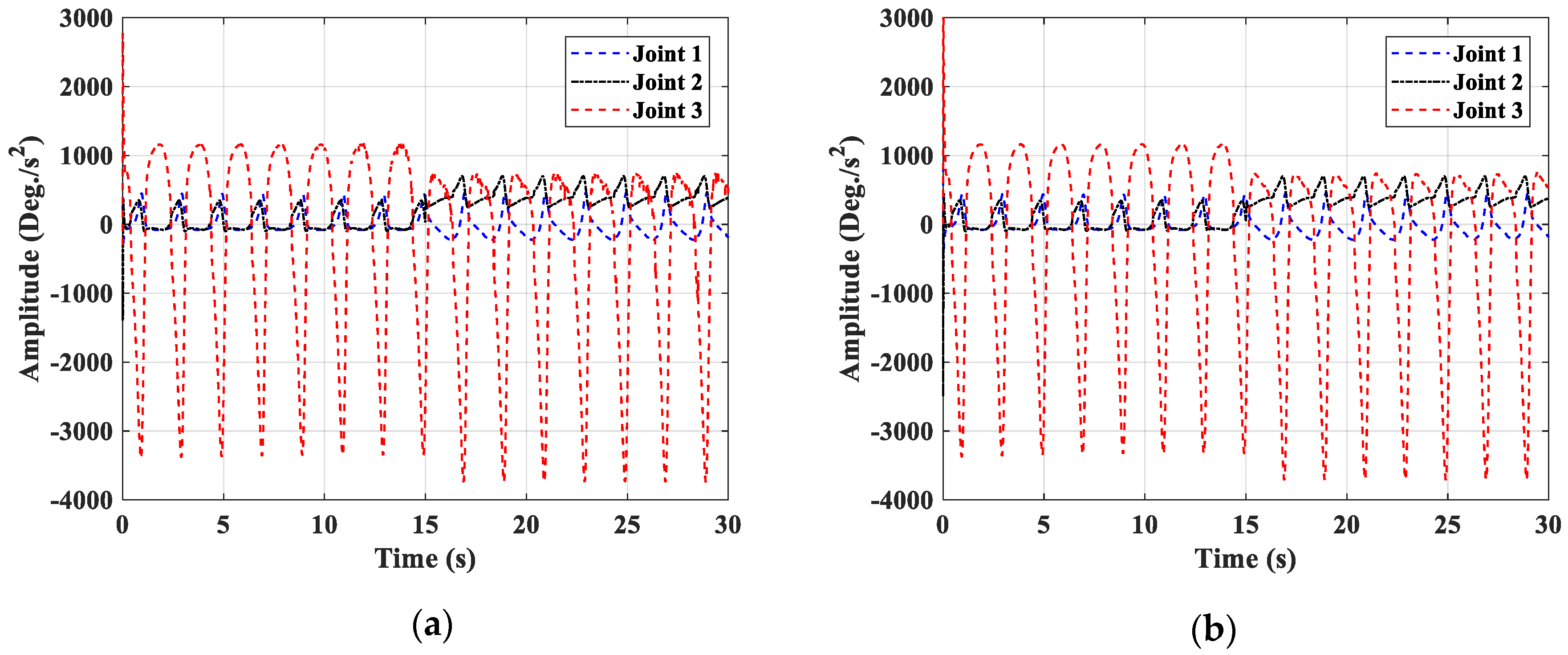
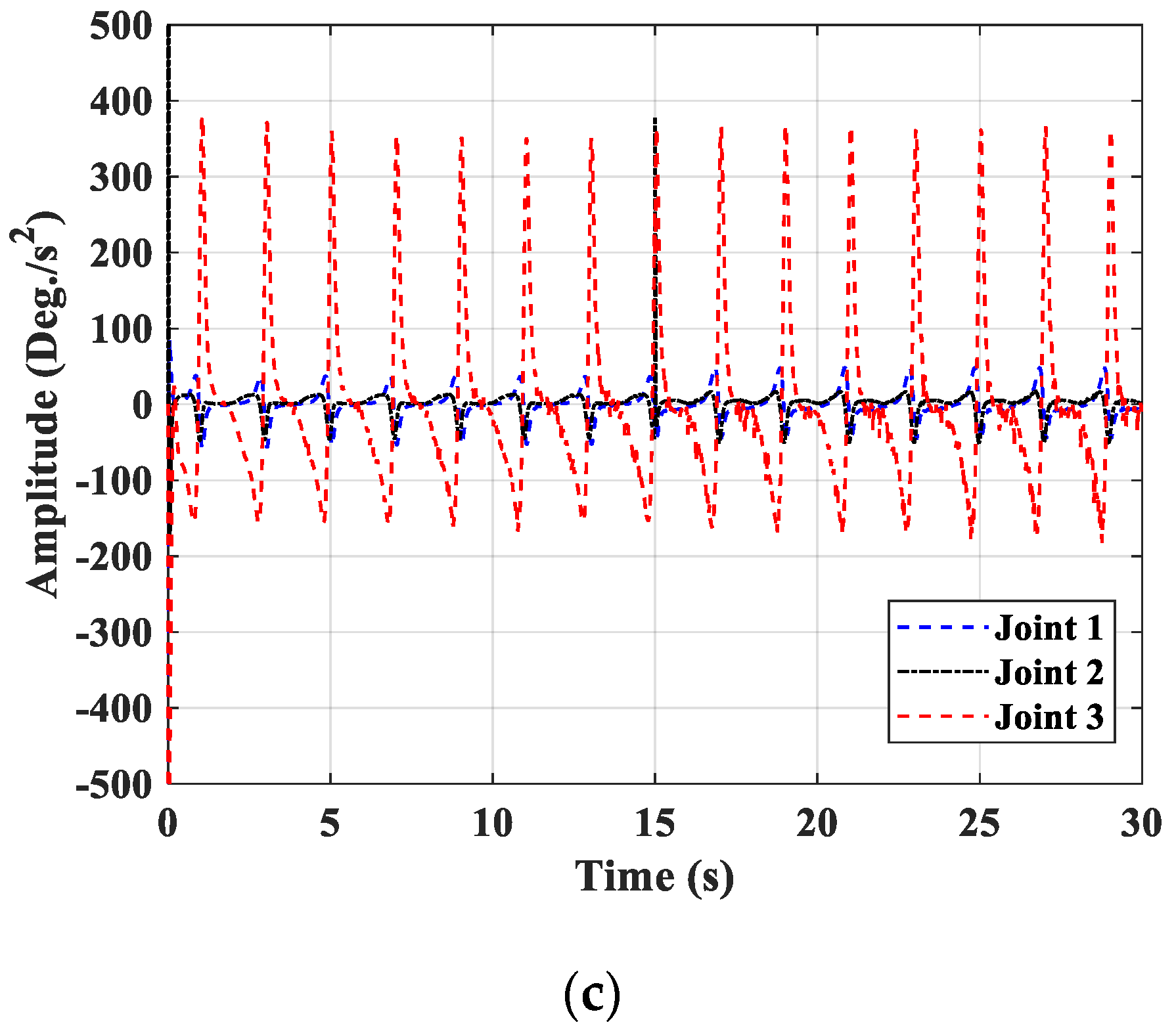
4.2.1. The First Simulation Case

Trajectories in the Cartesian coordinate with frequency at 0.1 Hz are generated for the 3-DOF planar manipulator. These references in the joint space are computed through the inverse-kinematic equations of the manipulator, which are presented in Figure 4. The references of joint 1, joint 2, and joint 3 are exhibited by a dashed black line, a dashed red line, and a dashed blue line, respectively. Figure 5 presents the output responses of the planar robot at the joint spaces. The results of the reference, backstepping control, LESOBC, and the proposed control are exhibited by dashed black lines, black lines, dashed dot black lines, and red lines, respectively. The boundaries of the output responses are presented by dashed dot black lines. From these results, we easily realize that the output responses of the backstepping control transgressed the output constraints. In order to exhibit the effectiveness of the proposed method, the differences between the references and output responses are presented in Figure 6. These results prove that the LESOBC and proposed control guarantee the satisfaction of the output responses with the output constraints under the presence of an unknown friction and external disturbance which arises at the 15th second.

The responses of the lumped uncertainties, $x_3$, at three joints are illustrated in Figure 7a with a dashed blue line, dashed dot black line, and dashed red line for joint 1, joint 2, and joint 3, respectively. In the first 15 s, the lumped uncertainties are unknown frictions at the joint space. In the last 15 s, an external force is applied at the end-effector along the x-axis. As a result, the uncertainties in each joint include not only the unknown friction but also the external disturbance. Therefore, they increased significantly and reduced the accuracy of the backstepping control. Figure 7b presents the estimated lumped disturbance, ${\widehat{x}}_3$, which is the result of the LESO. Comparing to the lumped disturbance in Figure 7a, the results of the estimated lumped disturbance in Figure 7b proved that the LESO has a limited bandwidth, which means it cannot approximate the disturbance at high frequency. The accuracy of the LESOBC and proposed control is improved significantly by using LESO to estimate the lumped disturbance. The estimated results of the LESO are presented in Figure 8. The estimated errors in position, velocity, and lumped disturbance are bounded.

Figure 9 respectively presents the torque responses of the BC, LESOBC, and the proposed control. The control responses of the BC are presented in Figure 9a when the input dead-zones are not compensated in the BC. In the LESOBC and proposed control, the torque responses are different from the BC because the input dead-zones in two controllers are compensated by the LESO. Finally, in order to evaluate the effectiveness of the proposed control in detail, the root mean square error (RMSE) is used for evaluating the responses of the three controllers. The results are shown in

Table 3. The root mean square error (RMSE) for the tracking errors of the manipulator at 0.1 Hz.

Controllers	1st Joint (Deg)	2nd Joint (Deg)	3rd Joint (Deg)
Backstepping control	24.5205	47.3142	43.4415
LESOBC	0.0055	0.008	0.0038
Proposed control	0.0001	0.0001	0.0001

.

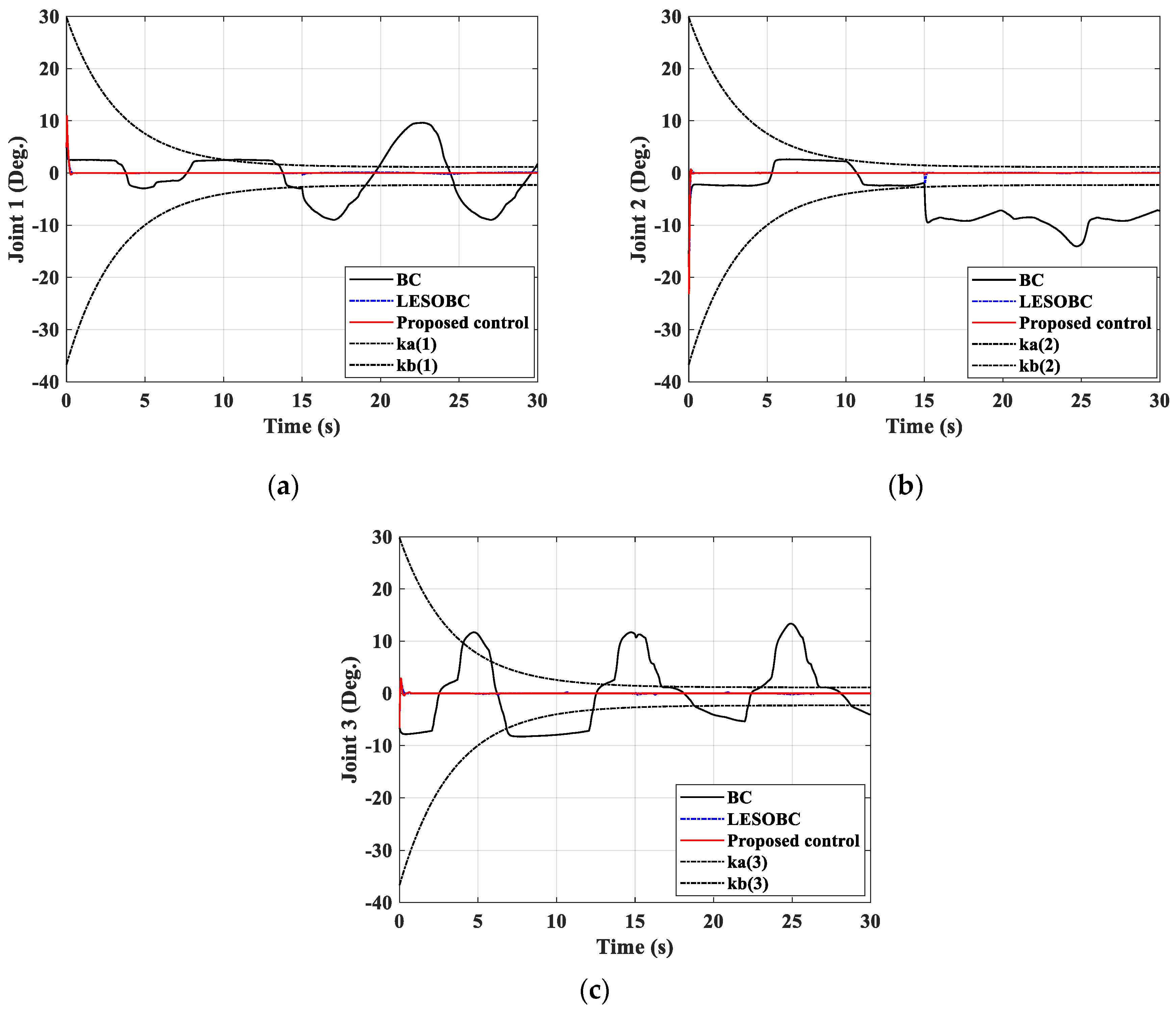
4.2.2. The Second Simulation Case

The trajectories in Cartesian coordinate with frequency at 0.5 Hz are applied for the 3-DOF planar manipulator. Similarly, compared to the previous simulation, the trajectories in the joint space of the manipulator are calculated by using the inverse-kinematic equations. Figure 10 presents the output error responses of three controllers at three joints. The output error responses of the backstepping control, LESOBC, and proposed control are respectively presented by black lines, dashed dot blue lines, and red lines. Additionally, the upper and lower error boundaries are plotted by the dashed dot black lines. The results in this figure show that the backstepping control still transgresses the constraints and the LESOBC begins breaking the output constraints because the accuracy of the LESOBC is improved by the LESO and it does not depend on the output boundaries. The proposed control is developed by integrating the output constraints into the control design. Therefore, its output responses are still guaranteed, although the working frequency increases. With this simulation, we see the effectiveness of the BLF in tackling the output constraints. The lumped uncertainties, in this case, are the unknown frictions in the first 15 s and a combination of the unknown frictions and external disturbances in the last 15 s.

The lumped disturbance responses, $x_3$, are presented in Figure 11a. Because the frequency of the trajectory is increased from 0.1 Hz to 0.5 Hz and the lumped uncertainties concern the velocity, the amplitude of the lumped disturbances increased if we compare it with the previous simulation. Figure 11b derives the estimated lumped disturbance, ${\widehat{x}}_3$, of the LESO.

The effectiveness of the LESO is presented in Figure 12, with the estimated error responses of the position, the velocity, and the lumped disturbance. The torque signals of the BC, LESOBC, and proposed control are exhibited in Figure 13. In the LESOBC and the proposed control, the control responses are also different from the BC because the input dead-zones are overcome by the LESO. Finally, in order to evaluate the effectiveness of the proposed control in detail, the root mean square error (RMSE) is used for evaluating the responses of the three controllers. The results are shown in

Table 4. RMSE for the tracking errors of the manipulator at 0.5 Hz.

Controllers	1st Joint (Deg)	2nd Joint (Deg)	3rd Joint (Deg)
Backstepping control	30.4138	52.7901	115.0904
ESOBC	0.2315	0.1260	0.6836
Proposed control	0.0159	0.0179	0.0197

.

In summary, the proposed controller that integrates the BLF-backstepping control and ESO is effective to control the manipulator at different motion frequencies (0.1 Hz and 0.5 Hz) under a bunch of problems as unknown friction, external disturbance, and unknown input dead-zone. The proposed controller outperforms the ESOBC and BC in terms of the RMSE as mentioned in Table 3 and Table 4, and especially entirely dominates the ESOBC at low frequency (0.1 Hz) and the BC at both low and high frequency, with respect to the prescribed-constraint performance as shown in Figure 6 and Figure 10.

5. Conclusions

This paper proposed an output feedback control via an extended state observer for an n-DOF robotic manipulator under the presence of unknown friction, external disturbances, input dead-zone, and the time-varying output constraints. These challenges are presented with n-DOF manipulator dynamics in mathematical equations. The proposed controller was developed from the LESO and the barrier Lyapunov function with the backstepping framework. The LESO estimated both the lumped disturbance and the unmeasured states in the robotic manipulator. Additionally, the BLF guaranteed that the output responses avoid violation of the constraints. Next, the Lyapunov approach was theoretically conducted to analyze the stability and robustness of the proposed control of the manipulator. Some simulations were conducted on the 3-DOF planar manipulator. The comparative results between the proposed control and the other controllers, such as backstepping control and the LESOBC, prove the superiority of the proposed control in improving accuracy against the lumped disturbances.

In future works, some advanced control can be developed from this algorithm to deal with other challenges such as finite-time convergence, the chattering effect, and input constraints, besides the output constraints. Some adaptive approximations can be investigated in this algorithm when the LESO is used as a fault detector or a force estimator for the manipulator.

References

1. Baek, J.; Kwon, W.; Kim, B.; Han, S. A Widely adaptive time-delayed control and its application to robot manipulators. IEEE Trans. Ind. Electron. 2018, 66, 5332–5342. [Google Scholar] [CrossRef]
2. Craig, J.J. Introduction to Robotics: Mechanics and Control; Pearson Prentice Hall: Upper Saddle River, NJ, USA, 2005; Volume 3. [Google Scholar]
3. Tran, D.T.; Truong, H.V.A.; Ahn, K.K. Adaptive backstepping sliding mode control based rbfnn for a hydraulic manipulator including actuator dynamics. Appl. Sci. 2019, 9, 1265. [Google Scholar] [CrossRef] [Green Version]
4. Truong, H.V.A.; Tran, D.T.; To, X.D.; Ahn, K.K.; Jin, M. Adaptive fuzzy backstepping sliding mode control for a 3-DOF hydraulic manipulator with nonlinear disturbance observer for large payload variation. Appl. Sci. 2019, 9, 3290. [Google Scholar] [CrossRef] [Green Version]
5. Tran, D.T.; Ba, D.X.; Ahn, K.K.; Thien, T.D. Adaptive backstepping sliding mode control for equilibrium position tracking of an electrohydraulic elastic manipulator. IEEE Trans. Ind. Electron. 2020, 67, 3860–3869. [Google Scholar] [CrossRef]
6. Duc-Thien, T. Adaptive sliding mode control with backstepping technique for hydraulic manipulator. In Proceedings of the 33rd Institute of Control Robotics and Systems, Buan, Korea, 17 May 2018. [Google Scholar]
7. Jung, S. Improvement of tracking control of a sliding mode controller for robot manipulators by a neural network. Int. J. Control. Autom. Syst. 2018, 16, 937–943. [Google Scholar] [CrossRef]
8. Chen, K.Y. Robust Optimal Adaptive Sliding Mode Control with the Disturbance Observer for a Manipulator Robot System. Int. J. Control. Autom. Syst. 2018, 16, 1701–1715. [Google Scholar] [CrossRef]
9. Nikdel, N.; Badamchizadeh, M.; Azimirad, V.; Nazari, M. Adaptive backstepping control for an n-degree of freedom robotic manipulator based on combined state augmentation. Robot. Comput. Manuf. 2017, 44, 129–143. [Google Scholar] [CrossRef]
10. Chang, W.; Li, Y.; Tong, S. Adaptive fuzzy backstepping tracking control for flexible robotic manipulator. IEEE/CAA J. Autom. Sin. 2018, 1–9. [Google Scholar] [CrossRef] [Green Version]
11. Park, S.; Lee, H.; Han, S.; Lee, J. Adaptive Fuzzy Super-twisting Backstepping Control Design for MIMO Nonlinear Strict Feedback Systems. Int. J. Control. Autom. Syst. 2018, 16, 1165–1178. [Google Scholar] [CrossRef]
12. Lv, W.; Wang, F.; Zhang, L. Adaptive fuzzy finite-time control for uncertain nonlinear systems with dead-zone input. Int. J. Control. Autom. Syst. 2018, 16, 2549–2558. [Google Scholar] [CrossRef]
13. He, W.; Huang, B.; Dong, Y.; Li, Z.; Su, C.Y. Adaptive neural network control for robotic manipulators with unknown deadzone. IEEE Trans. Cybern. 2017, 48, 2670–2682. [Google Scholar] [CrossRef] [PubMed]
14. Lin, C.H. Nonlinear backstepping control design of LSM drive system using adaptive modified recurrent laguerre orthogonal polynomial neural network. Int. J. Control. Autom. Syst. 2017, 42, 494–917. [Google Scholar] [CrossRef]
15. Lin, C.H.; Ting, J.C. Novel nonlinear backstepping control of synchronous reluctance motor drive system for position tracking of periodic reference inputs with torque ripple consideration. Int. J. Control. Autom. Syst. 2019, 17, 1–17. [Google Scholar] [CrossRef]
16. Yi, G.; Mao, J.; Wang, Y.; Guo, S.; Miao, Z. Adaptive tracking control of nonholonomic mobile manipulators using recurrent neural networks. Int. J. Control. Autom. Syst. 2018, 16, 1390–1403. [Google Scholar] [CrossRef]
17. Yao, J.; Jiao, Z.; Ma, D. Extended-state-observer-based output feedback nonlinear robust control of hydraulic systems with backstepping. IEEE Trans. Ind. Electron. 2014, 61, 6285–6293. [Google Scholar] [CrossRef]
18. Liu, J.; Gai, W.; Zhang, J.; Li, Y. Nonlinear adaptive backstepping with ESO for the quadrotor trajectory tracking control in the multiple disturbances. Int. J. Control. Autom. Syst. 2019, 17, 2754–2768. [Google Scholar] [CrossRef]
19. Wang, J.; Hung, J.Y. Adaptive Backstepping Control for an Underwater Vehicle Manipulator System Using Fuzzy Logic. In Proceedings of the IECON 2018—44th Annual Conference of the IEEE Industrial Electronics Society, Washington, DC, USA, 21–23 October 2018. [Google Scholar]
20. Wu, Y.; Huang, R.; Li, X.; Liu, S. Adaptive neural network control of uncertain robotic manipulators with external disturbance and time-varying output constraints. Neurocomputing 2019, 323, 108–116. [Google Scholar] [CrossRef]
21. Han, J. From PID to active disturbance rejection control. IEEE Trans. Ind. Electron. 2009, 56, 900–906. [Google Scholar] [CrossRef]
22. Tran, D.T.; Do, T.C.; Ahn, K.K. Extended high gain observer-based sliding mode control for an electro-hydraulic system with a variant payload. Int. J. Precis. Eng. Manuf. 2019, 20, 2089–2100. [Google Scholar] [CrossRef]
23. Jun, G.H.; Ahn, K.K. Extended-state-observer-based nonlinear servo control of an electro-hydrostatic actuator. J. Drive Control 2017, 14, 61–70. [Google Scholar]
24. Chen, H.T.; Song, S.M.; Zhu, Z.B. Robust Finite-time Attitude Tracking Control of Rigid Spacecraft Under Actuator Saturation. Int. J. Control. Autom. Syst. 2018, 16, 1–15. [Google Scholar] [CrossRef]
25. Mario, R.N.; Hebertt, S.R.; Rubén, G.M.; Alberto, L.J. Active Disturbance Rejection Control of the Inertia Wheel Pendulum through a Tangent Linearization Approach. Int. J. Control. Autom. Syst. 2019, 17, 18–28. [Google Scholar] [CrossRef]
26. Zhao, Y.; Yu, J.; Tian, J. Robust output tracking control for a class of uncertain nonlinear systems using extended state observer. Int. J. Control. Autom. Syst. 2017, 15, 1227–1235. [Google Scholar] [CrossRef]
27. Ren, B.; Ge, S.S.; Tee, K.P.; Lee, T.H. Adaptive neural control for output feedback nonlinear systems using a barrier lyapunov function. IEEE Trans. Neural Netw. 2010, 21, 1339–1345. [Google Scholar] [CrossRef]
28. Li, Y.; Yang, C.G.; Yan, W.; Cui, R.; Annamalai, A. Admittance-based adaptive cooperative control for multiple manipulators with output constraints. IEEE Trans. Neural Netw. Learn. Syst. 2019, 30, 3621–3632. [Google Scholar] [CrossRef] [Green Version]
29. Wang, C.; Wu, Y.; Yu, J. Barrier Lyapunov functions-based adaptive control for nonlinear pure-feedback systems with time-varying full state constraints. Int. J. Control. Autom. Syst. 2017, 15, 2714–2722. [Google Scholar] [CrossRef]
30. He, W.; David, A.O.; Yin, Z.; Sun, C. Neural network control of a robotic manipulator with input deadzone and output constraint. IEEE Trans. Syst. Man Cybern. Syst. 2016, 46, 759–770. [Google Scholar] [CrossRef]
31. Guo, Q.; Liu, Y.; Wang, Q.; Jiang, D. Adaptive neural network control of Two-DOF robotic arm driven by electro-hydraulic actuator with output constraint. In Proceedings of the IET Conference, Guiyang, China, 19–22 June 2018; p. 7. [Google Scholar]
32. Zhou, Q.; Wang, L.; Wu, C.; Li, H.; Du, H. Adaptive fuzzy control for nonstrict-feedback systems with input saturation and output constraint. IEEE Trans. Syst. Man Cybern. Syst. 2017, 47, 1–12. [Google Scholar] [CrossRef]
33. Edalati, L.; Sedigh, A.K.; Shooredeli, M.A.; Moarefianpour, A. Adaptive fuzzy dynamic surface control of nonlinear systems with input saturation and time-varying output constraints. Mech. Syst. Signal. Process. 2018, 100, 311–329. [Google Scholar] [CrossRef]
34. Mien, V.; Mavrovouniotis, M.; Ge, S.S. An adaptive backstepping nonsingular fast terminal sliding mode control for robust fault tolerant control of robot manipulators. IEEE Trans. Syst. Man Cybern. Syst. 2018, 49, 1448–1458. [Google Scholar] [CrossRef] [Green Version]
35. Yang, H.; Sun, J.; Xia, Y.; Zhao, L. Position control for magnetic rodless cylinders with strong static friction. IEEE Trans. Ind. Electron. 2018, 65, 5806–5815. [Google Scholar] [CrossRef]
36. Tran, D.T.; Jin, M.; Ahn, K.K. Nonlinear extended state observer based on output feedback control for a manipulator with time-varying output constraints and external disturbance. IEEE Access 2019, 7, 156860–156870. [Google Scholar] [CrossRef]
37. Guo, Q.; Zhang, Y.; Celler, B.G.; Su, S. Backstepping control of electro-hydraulic system based on extended-state-observer with plant dynamics largely unknown. IEEE Trans. Ind. Electron. 2016, 63, 6909–6920. [Google Scholar] [CrossRef]
38. Yu, J.; Zhao, L.; Yu, H.; Lin, C. Barrier Lyapunov functions-based command filtered output feedback control for full-state constrained nonlinear systems. Automatica 2019, 105, 71–79. [Google Scholar] [CrossRef]
39. Huang, A.C.; Chien, M.C. Adaptive Control of Robot Manipulators: A Unified Regressor-Free Approach; World Scientific: Singapore, 2010. [Google Scholar]
Figure 1. Dead-zone model.
Electronics 09 01355 g001
Figure 2. Structure of the proposed control. BLF = barrier Lyapunov function; n-DOF = n-degree-of-freedom.
Electronics 09 01355 g002
Figure 3. Structure of the 3-DOF manipulator.
Electronics 09 01355 g003
Figure 4. References of the 3-DOF planar manipulator in joint space at 0.1 Hz.
Electronics 09 01355 g004
Figure 5. Output responses of the three controllers in (a) joint 1; (b) joint 2; and (c) joint 3 at 0.1 Hz.
Electronics 09 01355 g005
Figure 6. Error responses of the three controllers in (a) joint 1; (b) joint 2; and (c) joint 3 at 0.1 Hz.
Electronics 09 01355 g006
Figure 7. Lumped disturbance response of the planar manipulator at 0.1 Hz: (a) lumped disturbance and (b) estimated lumped disturbance.
Electronics 09 01355 g007
Figure 8. Estimated error results of the extended state observer at 0.1 Hz: (a) position error, (b) velocity error, and (c) lumped uncertainties errors.
Electronics 09 01355 g008
Figure 9. Control signals of the proposed control at 0.1 Hz: (a) backstepping control; (b) LESOBC; and (c) proposed control.
Electronics 09 01355 g009
Figure 10. Error responses of three controllers in: (a) joint 1; (b) joint 2; and (c) joint 3 at 0.5 Hz.
Electronics 09 01355 g010
Figure 11. Lumped disturbance response of the planar manipulator at 0.5 Hz: (a) lumped disturbance and (b) estimated lumped disturbance.
Electronics 09 01355 g011
Figure 12. Estimated error results of the extended state observer at 0.5 Hz: (a) position error, (b) velocity error, and (c) lumped uncertainties errors.
Electronics 09 01355 g012aElectronics 09 01355 g012b
Figure 13. Control signals of the proposed control at 0.5 Hz: (a) backstepping control; (b) LESOBC; and (c) proposed control.
Electronics 09 01355 g013