Abstract
We address a class of authentication protocols called “HB” ones and the man-in-the-middle (MIM) attack, reported at the ASIACRYPT conference, called OOV-MIM (Ouafi-Overbeck-Vaudenay MIM). Analysis of the considered attack and its systematic experimental evaluation are given. It is shown that the main component of OOV-MIM, the algorithm for measuring the Hamming weight of noise vectors, outputs incorrect results as a consequence of the employed approximation of the probability distributions. The analysis reveals that, practically, the only scenario in which the OOV-MIM attack is effective is the one in which two incorrect estimations produced by the algorithm for measuring the Hamming weight, when coupled, give the correct result. This paper provides additional insights into the OOV-MIM and corrected claims about the performance/complexity showing that the performances of the considered attack have been overestimated, i.e., that the complexity of the attack has been underestimated. Particularly, the analysis points out the reasons for the incorrect claims and to the components of the attack that do not work as expected.
1. Introduction
RFID (radio frequency identification) is a technology that uses electromagnetic fields to detect, identify, and track objects. It has found its application in various fields, such as supply chain management, toll collection, access control, animal identification, and more. The necessity to provide some level of security and privacy in RFID systems, on one hand, and inherent constraints of the RFID devices, on the other, have made RFID authentication a very active and challenging research subject [1,2,3,4]. As a solution, a number of lightweight authentication protocols have been proposed, and one of the significant families of protocols among these is the HB family. The HB family of authentication protocols has received a great deal of attention as a cryptographic technique for authentication. One of the reasons is that its security is based on the hardness of the so-called learning parity with noise (LPN) problem, which is shown to be NP-complete (see [5]). This security means that if the adversary can break the protocol (in a certain scenario), the adversary is also capable of solving a hard problem (employing appropriate reduction technique). The fact that the LPN problem could be easily implemented in hardware since it uses XOR and AND operations only, makes it particularly suitable for applications in lightweight cryptography.
The HB family of authentication protocols originates from the HB protocol [6], proven to be secure against passive attacks where the adversary is capable of eavesdropping the communication sessions between the tag and the reader. However, the HB protocol appears to be vulnerable against an active adversary who can also interrogate the tag by impersonating the reader. To prevent this kind of attack, another protocol, HB+ has been proposed (see [7,8]) secure against the considered attack. Later on, it was found that the HB+ protocol could be broken by a stronger adversary who can modify the messages sent by the reader (called GRS-MIM attack) [9]. After that, a number of variants of the HB+ protocol were proposed in order to hinder the GRS-MIM attack (e.g., HB++ [10], HB-MP [11]), but all of them appeared to be vulnerable, until the HB# and Random-HB# protocols [12] were introduced and proven to be secure against the GRS-MIM attack. A follow-up was that Ouafi et al. [13] have introduced a more general MIM attack which can break HB# and Random-HB#. This attack has been referred to as the OOV attack, and it presupposes an adversary that can modify the messages exchanged in both directions between the tag and the reader. An improvement of Random-HB#, known as HB-MAC [14], was later proposed. In parallel, improved successors of HB-MP were introduced: HB-MP+ [15], HB-MP++ [16], HB-MP* [17]. The HB family also includes Trusted-HB [18], NLHB [19], HBN [20], and GHB# [21], as well as HB+PUF [22], PUF-HB [23], and Tree-LSHB [24,25]. Avoine et al. [1] emphasize that the OOV attack remains one of the keystones in the analysis of any new HB-like authentication scheme.
Tomović et al. [26] proposed the NHB# protocol, a modification of HB#, which uses randomized selection of secret matrices, in order to impede this kind of attack. Later, it was shown that the NHB# protocol, as well, can be broken by an adversary who employs the OOV attack as its component [27], but the complexity of such an attack on NHB# is significantly higher than the one for HB#. The security analysis of the NHB# protocol presented by Tomović et al. [27], does not go into a detailed evaluation of the OOV attack and its correctness, but rather observes the OOV attack in a “black-box” manner and refers to the results about its efficiency given in [13] (see Figure 1). By examining the papers citing the OOV attack [13], it can be found they take the same “black-box” approach, i.e., the do not attempt a replication study nor reconsider the claims about the complexity of the OOV attack.
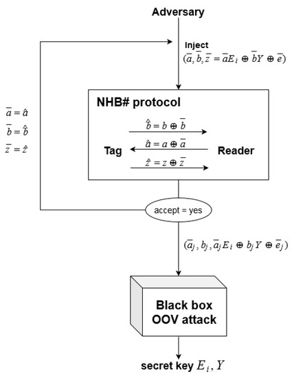
Figure 1.
The OOV-MIM attack is used as a “black box” component of the attack on the NHB# protocol.
Motivation for the Work. The MIM attack is recognized as a very important one for security evaluation considerations of authentication protocols. The OOV-MIM attack reported in [13] is an important instantiation of MIM attacks and it has received significant research attention. We have implemented the OOV-MIM attack for practical security evaluation of the NHB# authentication scheme and the performed experiments have shown a discrepancy between the expectations based on the performance claimed in [13] and the results obtained in the experiments. Consequently, it has appeared as an interesting issue to perform a systematic experimental evaluation of the attack proposed in [13] and to provide more insights about the considered OOV-MIM attack approach. It should be noted that not only the feasibility of an attack, but also its performances, appear as very important in security evaluation scenarios. In particular, the OOV-MIM requires a certain (large) number of modifications, i.e., interruptions of authentication sessions to be executed, and from a practical point, this number determines the complexity of the attack and strongly implies its practical impact. In some scenarios requirement for 50% larger sample could be a significant limitation. To the best of our knowledge, there have been no reports on experimental re-evaluation of the theoretical analysis and the claimed complexity of the OOV-MIM attack given in [13].
Summary of the Results. The paper provides significant novel insights into the OOV-MIM attack through in-depth analysis that includes: (i) the analysis of the employed technical elements, (ii) simulation of the entire algorithm, and (iii) its performance re-evaluation. We show that the core component of the OOV-MIM attack (Algorithm 1, which measures the Hamming weight of a noise vector) has the high probability of an incorrect output. Nevertheless, an interesting finding is that coupling of two incorrect outputs can result in an unplanned neutralization of the errors, yielding a correct outcome. Furthermore, the analysis shows that, practically, the only scenario in which the OOV-MIM attack is effective is the one in which the errors mutually neutralize each other. The results justify that the claimed performances of the OOV-MIM attack are overestimated, i.e., the complexity of the attack execution is significantly higher in comparison with the claimed complexity which could imply significant impact in certain practical applications of the attack.
Organization of the Paper.Section 2 provides the background elements. An overview of the performed analysis is given in Section 3. Experimental evaluation of the OOV-MIM attack and a detailed analysis of the result are given in Section 4 and Section 5. Finally, some concluding remarks are given in Section 6.
2. Background
Here, we briefly review the HB# and Random-HB# protocols from [12], and the mechanism of the MIM attack against them, which has been introduced in [13]. The following notation is used throughout the remainder of the paper:
| Notation | Description |
| The set of all -dimensional binary vectors | |
| The set of all -dimensional binary matrices | |
| The operation of sampling a value from the uniform distribution on the finite set | |
| i-th bit of vector x | |
| The Bernoulli distribution with parameter | |
| The bit follows the Bernoulli distribution , i.e., and | |
| The operation of randomly choosing vector among all the vectors of length , such that , for | |
| The bitwise exclusive OR (XOR) operation of vectors | |
| The Hamming weight of binary vector , which is the number of non-zero bits | |
| The probability of an event | |
| Normal distribution with mean and standard deviation | |
| The standard normal cumulative distribution function | |
| The complementary error function | |
| The probability of accepting a vector , whose Hamming weight is , in HB# and Random-HB#, after adding random noise to , i.e., | |
| The approximation for used in the OOV paper [13] which is defined as | |
| The experimentally-obtained value for |
2.1. Review of the HB# and Random-HB# Protocols
In Random-HB#, the tag and the reader share some secret, random matrices and perform the following authentication process (see Figure 2): first, the tag sends a random vector to the reader (a blinding vector) and the reader responds with a random vector (a challenge). Then the tag computes , where is a noise vector whose bits follow the Bernoulli distribution independently with some coefficient , and sends to the reader. Finally, the reader performs the validation of the tag: the authentication is successful if and only if , for a given threshold value . HB# has the same construction as Random-HB# with only difference in that the secret matrices and are Toeplitz matrices.
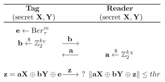
Figure 2.
HB# and Random-HB# authentication protocols [13].
2.2. The Man-In-The-Middle Attack against HB# and Random-HB#
Random-HB# and HB# were formally proven to be secure against a special GRS-MIM adversary. In the first phase of the attack, the adversary is capable of eavesdropping the communication between the honest tag and the reader (including the reader’s decision on the authentication success) and modifying the messages sent from the reader to the tag. After gathering enough information, the adversary tries to authenticate itself to the reader by impersonating the valid tag.
However, Ouafi et al. [13] have reported a more powerful MIM attack (the OOV attack), where the adversary has the ability to change all the messages exchanged between the tag and the reader. The main idea behind this attack is that the adversary repeatedly corrupts authentication sessions between the honest tag and the reader by replacing triplets with each time, and to count the number of successful authentications afterwards. This number, i.e., the acceptance rate in these corrupted sessions, leaks the critical information for recovering the secret keys.
More precisely, the authors in [13] notice that the probability of acceptance in a corrupted session is , where . Then they observe that if is the number of successful authentications in corrupted sessions using a triplet , it holds that:
The joint approximation provides the adversary with enough means to estimate the Hamming weight of the noise vector using the empirically obtained frequency , for large enough (see Algorithm 1). The adversary then recovers by flipping its bits one-by-one and measuring its weight after flipping: if the weight of has increased, the original bit was 0, otherwise the bit was 1 (see Algorithm 2). By recovering , the adversary discovers the linear combination . Since one triplet forms a system of equations, in order to obtain a full linear system with unknown and the adversary repeats the previous process times on linearly independent pairs , where is the number of secret bits, which is for HB#, and for Random-HB#. Finally, the adversary recovers the secret and as the solution to this system.
The illustration of the OOV attack (Figure 3), and the pseudocodes of Algorithm 1 and Algorithm 2 from [13] are given below.
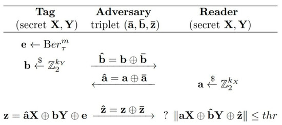
Figure 3.
Man-in-the-middle OOV attack against the HB# and Random-HB# authentication protocols [13].
Here we denote by as the messages created and sent by the tag and the reader, and by as the corresponding messages they received after the adversary’s intervention.
| OOV Algorithm 1 [13]: Approximating= |
|
Algorithm 1 uses as input a triplet obtained by eavesdropping a previous authentication session between the honest tag and the reader. The output is the Hamming weight of the noise vector . The algorithm iterates through intercepted authentications, where is big enough to accurately recover . That is, with high probability if where:
as derived in [13].
| OOV Algorithm 2 [13]: Getting linear equations for secret keys |
|
Algorithm 2 takes as input ), a triplet obtained by eavesdropping a communication session between the honest tag and the reader, and the expected weight of , and it recovers a linear combination of the secret keys
Ouafi et al. [13] show that the overall complexity of the attack can be expressed in terms of the number of intercepted authentication sessions between the tag and the reader. The optimal weight of the noise vector is the weight which minimizes the number of these authentication sessions in Algorithm 1, i.e., . In order to achieve that the input triplet ) in Algorithm 1 contains noise vector whose expected weight is optimal, they manipulate the number of errors (i.e., one-bits) in the observed noise vector by flipping the adequate number of bits.
3. Overview of the Performed Analysis and Results
This section provides an overview of the in-depth analysis of the OOV-MIM attack presented in Section 4 and Section 5. Our analysis includes: (i) examination of OOV Algorithm 1, which is the core element of the attack; (ii) reconstruction, simulation, and analysis of the full attack; and (iii) correction of the algorithm performance/complexity. Accordingly, this section yields an overview of the obtained results and additional insights into the OOV-MIM attack. The findings of this paper are summarized in the five statements (a)–(e) below which not only correct the incorrect claims about the attack efficiency and complexity, but also point out to the components of the attack that do not work as expected, and the reasons for their faulty behavior:
- (a)
- Algorithm 1 outputs incorrect results. As the first step, we investigate correctness and efficiency of Algorithm 1 for estimating the Hamming weight of a noise vector, which is a fundamental operation and determines complexity of the attack. As in the OOV-MIM attack [13], in our focus are the noise vectors with the optimal Hamming weight, since the complexity of a key recovery is lowest for such vectors. Experimental results for a standard parameter set show that Algorithm 1 has a tendency to estimate the weight of the observed noise vector lower than the actual value. Moreover, by increasing n, instead of better precision, the number of erroneous weight estimates increases as well. The detailed results are presented in Section 4.2. We show the difference between the acceptance rate expected values claimed in [13] and our experimental results. In addition, we demonstrate that, for very large n, contrary to what is expected, the percentage of correctly estimated weights is particularly low for the vectors closer to the optimal weight. 99% of the noise vectors weights that are being measured by Algorithm 1 for the analyzed standard parameter set fall into the interval [60,95] and only 5.38% of them are correctly guessed. We show that the probability of the correct weight estimate is significantly lower than the claimed one. Section 5.1 provides analytical and illustrative numerical consideration of the probability of correct weight estimation.
- (b)
- Employment of Algorithm 1 in the OOV-MIM attack is such that two incorrect results of Algorithm 1 can cancel each other and yield the correct output of Algorithm 2, i.e., recovery of the noise vector. We show that when the noise vector weight is correctly estimated, the probability of a noise vector recovery and consequently key recovery is negligible. On the other hand, we identify an unintended feature that the error in the weight estimation and the error in the bit guessing procedure can neutralize each other and give correct bit estimate as a result. Namely, our analysis shows that the attacker can incorrectly estimate the weight, but correctly recover all the bits, and discover that the observed vector has one more “1” than expected, having in mind the initial noise vector’s weight estimate. On the other hand, a more severe situation regarding the correct key recovery occurs when the attacker correctly guesses the weight, which happens with a probability that is not negligible. Figure 4 illustrates this interesting behavior and shows actual probabilities of a noise vector recovery for a standard parameter set. Section 5.2, Section 5.3, Section 5.4 and Section 5.5 provide analytical and illustrative numerical analysis of the probabilities for correct recovery of the noise bits in the four basic scenarios.
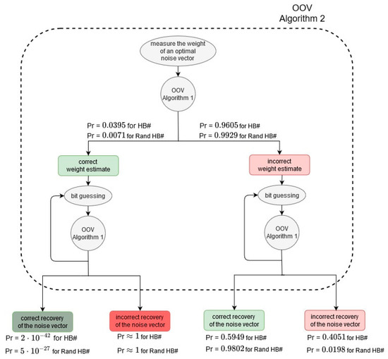 Figure 4. Probability of correct noise vector recovery (Algorithm 2) in the OOV attack depends on mutual cancelation of errors produced by Algorithm 1. If the weight of a noise vector has been correctly measured, the probability that Algorithm 2 will correctly recover the bits of the vector is negligible. Practically, the only way Algorithm 2 can recover the noise vector is that to initially incorrectly estimate its weight, and then rely on the fact that the error made in the bits guessing procedure can neutralize the previous error.
 - (c)
- Findings (a)–(b) appear as a consequence of employing an inappropriate approximation of the probability distributions. The difference between the acceptance rate expected values as given in [13] and the experimentally obtained ones is analyzed in Section 4.2. The results show that as we are moving away from the optimal weight, the two curves get closer, but it is important to notice that in the central part of the graph, around the optimal weight, the curves are the most distant. This explains the observed tendency of the OOV Algorithm 1 to estimate noise weight as 1 lower than the actual value, when the weight is close to the optimal.
- (d)
- The complexity of the attack has been underestimated, i.e., its performances have been overestimated.Section 5.6 gives the analytical and numerical evaluation of the key recovery probability. We show how the probability of key recovery increases with an increase of the number of intercepted authentication sessions n which, consequently, implies the increase of the total (key recovery) complexity as well. In order to achieve the success rate claimed in [13], it is necessary to significantly increase the overall complexity budget of the algorithm. In the case of the HB# protocol it is necessary to use n = 1634 instead of 1382 (increase of 18%), and in the case of the Random-HB# protocol it is necessary to use n = 4196 instead of 2697 (increase of 55%).
- (e)
- Employment of block optimization in the advanced version of the OOV-MIM attack leads to precision loss. Ouafi et al. [13] propose an optimization of the basic, bit-by-bit version of the attack. The optimization is based on splitting the vectors into blocks and measuring weight of blocks instead of individual bits. This way, the total number of measurements, and consequently the complexity of the attack, decreases. However, we experimentally demonstrate that this optimization leads to deterioration of the key recovery probability. We also provide an adequate rationale and explanation for this finding.
4. Analysis of Algorithm 1—The Core Component of the Attack against the HB# Protocols
We have implemented and simulated the core component of the OOV attack (Algorithm 1) in MATLAB (The MathWorks Inc., Natick, Massachusetts). The results reveal incorrectness regarding the output of Algorithm 1, i.e., the Hamming weight estimate. This section provides details about initial experimental evaluation of Algorithm 1.
4.1. Acceptance Rates and the OOV Weight Estimates
The authors in [13] point out two probabilistic approximations:
and afterwards, they join them into one approximation which is used to estimate the weight in Algorithm 1:
The first approximation is a direct consequence of the law of large numbers. The second one follows from the central limit theorem, where is a sum of independent Bernoulli random variables.
4.2. Erroneous Weight Estimate Using the OOV Algorithm
We conducted a series of experiments simulating the OOV attack proposed by Ouafi et al. [13]. First, we investigated the correctness and efficiency of Algorithm 1 for measuring the Hamming weight of a noise vector, which is a fundamental operation and complexity unit of the attack. Our focus was initially set on the noise vectors with the optimal Hamming weight. The optimal Hamming weight requires the minimal number n of intercepted authentication sessions (message modifications). The optimal weight is, consequently, such that the acceptance rate is (closest to) . For parameter set II, the OOV paper marks weight 77 as optimal. Experimental results show that Algorithm 1 has a tendency to estimate the weight of the observed noise vector as lower than the actual value. Specifically, the noise vectors of the weight 77 were estimated as 76, those of the weight 78 as 77, and so on. We tested the algorithm with different number of modifications , in order to confirm whether the OOV estimate for was large enough, i.e., if the detected error, was a consequence of underestimating . For each , 100,000 noise vectors with Hamming weight of 78 were generated and their weight was estimated using Algorithm 1. The experiments showed that by increasing , instead of better precision, the number of erroneous weight estimates increased as well. The results are presented in Table 1 and Figure 5.

Table 1.
The ratio of correct weight estimates gets smaller as the number of modifications increases.
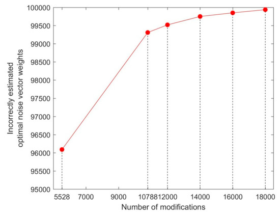
Figure 5.
The increase in erroneous weight estimates with the increase of number of modifications. The observed sample consists of 100,000 noise vectors of the Hamming weight 78.
From Table 1 we also see that the empirical probability of successful weight estimation for noise vectors of the optimal weight significantly deviates from the probability claimed in [13] which is equal to , i.e., for the HB# protocol the claimed precision is 0.9986, and the empirical precision is 0.0391; for Random-HB# the claimed precision is 0.9999923, and the empirical precision is 0.0069.
Since the quality of the weight guessing procedure worsened as the number of modifications increased, we suspected that the problem may lay in the OOV acceptance rates. Figure 6 shows the difference between the acceptance rate expected values as given in [13] and the experimental results. The results show that as we are moving away from the optimal weight, the two curves get closer, but it is important to notice that in the central part of the graph, around the optimal weight, the curves are the most distant (see also Table 2). This difference explains the observed tendency of the OOV Algorithm 1 to estimate noise weight as 1 lower than the actual value, when the weight is close to the optimal.
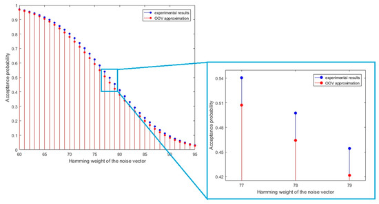
Figure 6.
Divergence between the OOV approximation and the experimental results of the acceptance rates for the noise vectors with the Hamming weight between 60 and 95. The detected divergence causes the OOV algorithm to make erroneous weight estimates.
Table 2.
Difference between the OOV approximation and the experimental acceptance rates for the noise vectors with the Hamming weight close to .
As mentioned earlier, the optimal weight is the one for which is closest to . It should be noted that this stands for the weight 78, and not 77, as stated in [13].
Further on, we have analyzed performance of the OOV weight estimate algorithm for noise vectors of different Hamming weights. Since almost all (~99%) noise vectors have the Hamming weight between 60 and 95 (this is after flipping bits in order to obtain a vector of the optimal weight from a vector of expected weight), we have focused on that interval and applied the OOV algorithm for weight estimate on a set of 20,000 randomly generated vectors. We have used 18,000 modifications which should give high success rate. Figure 7 shows that the percentage of correctly estimated weights is particularly low for the vectors closer to the optimal weight. Only 5.38% of the noise vector weights from the interval [60,95] are correctly guessed. This is in accordance and further confirms the previously observed deviation of the experimentally-obtained values shown in Figure 6 from the OOV approximation.
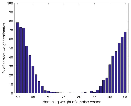
Figure 7.
Success rate of the OOV weight estimate algorithm for the noise vectors whose Hamming weight is between 60 and 95. The number of modifications is set to 18,000.
5. Re-Evaluation of the Man-In-The-Middle Attack against HB# and Random-HB# Protocols
Algorithm 1 for weight estimation is used multiple times in the OOV attack. First, it is used for estimating the weight of the observed noise vector. Thereafter, the same algorithm is used to discover bits of that vector. In this section we will elaborate on how the approximation used in the algorithm affects the recovery of the bits in the noise vector(s) and the overall key recovery. The results of our analysis refute the claims about the algorithm correctness, efficiency, and complexity given by Ouafi et al. [13]. Specifically, we evaluate the probability of the correct noise weight estimate, and further analyze how (in)correct weight estimate affects bit guessing. As in the OOV paper, our focus will be on the noise vectors with the optimal Hamming weight, since the complexity of a key recovery is lowest for such vectors. We show that the probability of the correct weight estimate is significantly lower than the probability of an error. We also show that when the weight is correctly estimated, the probability of the noise vector recovery (and consequently key recovery) is negligible (see Table 3).
Table 3.
Probability of successful noise vector recovery for HB# and Random-HB# protocols using the OOV algorithm, depending on the correctness of the initial weight estimate. Paradoxically, a noise vector can effectively be recovered only if its weight has initially been incorrectly estimated.
Further, we study how the error in the weight estimate and the error in the bit guessing can unintendedly neutralize each other and produce a correct bit estimate. Nevertheless, in order to achieve the success rate claimed in [13], it will be necessary to significantly increase the overall complexity of the algorithm. We also show that the optimized (block-by-block) version of the algorithm cannot be applied straightforwardly with the same number of modifications that is used in the non-optimized (bit-by-bit) version, since that leads to deterioration in the key recovery success rate.
5.1. The Probability of Correct Weight Estimate
First, we determine the probability that an attacker will correctly guess the weight of a noise vector using the OOV algorithm, when the weight is optimal, i.e., equal to 78. For modifications, the number of acceptances follows a binomial distribution, as it a sum of independent Bernoulli random variables, each with the same parameter . From the central limit theorem, will follow a normal distribution:
In order to evaluate the probability that the attacker will correctly guess the weight, we use experimentally obtained value for , i.e., .
However, the OOV attack observes the “shifted” distribution (see Figure 8), and concludes that the noise vector’s weight is 78 iff:
and:
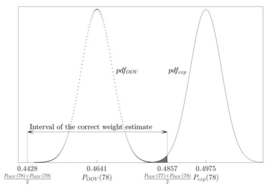
Figure 8.
The probability of correct weight estimate: When the weight of the observed noise vector is optimal (=78), the experimental acceptance rate follows the distribution , while the OOV algorithm uses the approximation ; the application of this approximation leads to high error rate in the weight estimation process.
Since follows the distribution (9), the probability that it falls into the interval : is
Table 4 shows the probability that the OOV algorithm will correctly estimate the weight of a noise vector whose weight is optimal, i.e., equal 78. We can see how this probability changes as increases. For each we provide analytical value obtained from the Formula (12) as well as the value from the experimental results.
Table 4.
Probability that the OOV algorithm will correctly estimate the weight of the noise vector whose weight is optimal (=78). Both analytically and experimentally obtained results demonstrate the algorithm has exceptionally low accuracy.
Based on the weight estimate, each bit of the noise vector is guessed. Hereinafter, we will analyze the error probability in the bit guessing process depending on the (in)correct weight estimate.
5.2. The Probability of an Incorrect 0-bit Guess when the Weight Estimate Is Correct
In the case when the observed bit is zero, after flipping it, the ratio follows the normal distribution:
In order to evaluate the probability that the attacker will incorrectly guess the bit, we use experimentally obtained value for , i.e., .
When the OOV algorithm correctly estimates the weight of the observed noise vector as 78, it will conclude that the flipped bit is zero iff (see Figure 9):
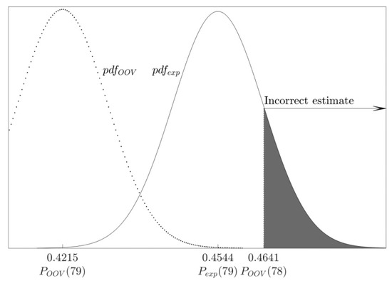
Figure 9.
The probability of an incorrect 0-bit guess when the weight estimate is correct: After flipping a 0-bit, acceptance rate follows the distribution ; knowing the weight of the noise vector (=78), the OOV algorithm estimates a bit as 0 iff
Since follows the distribution (13), the probability of an error, i.e., that the bit will be wrongly evaluated as 1, is:
Table 5 shows the probability that the OOV algorithm will wrongly estimate a zero-bit as a one-bit, when the noise vector weight is correctly estimated as 78. We can see how this probability changes as increases. For each we provide analytical value obtained from Formula (15) as well as the value from the experimental results. The error rates are too high and make it practically impossible to successfully recover the noise vector, as we will show in Section 5.6.
Table 5.
Probability that the OOV algorithm will incorrectly estimate a zero bit of the noise vector whose weight is correctly estimated as 78.
5.3. The Probability of an Incorrect One-Bit Guess when the Weight Estimate Is Correct
In the case when the observed bit is one, after flipping it, the ratio follows the normal distribution:
In order to evaluate the probability that the attacker will incorrectly guess the bit, we use experimentally obtained value for , i.e., .
When the OOV algorithm correctly estimates the weight of the observed noise vector as 78, it will conclude that a bit is one iff (see Figure 10):
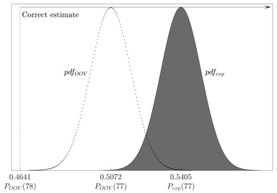
Figure 10.
The probability of an incorrect one-bit guess when the weight estimate is correct: After flipping a one-bit, acceptance rate follows the distribution ; knowing the weight of the noise vector (=78), the OOV algorithm estimates a bit as 1 iff
Since follows the distribution shown in Equation (16), the probability of an error, i.e., that the bit will be wrongly evaluated as zero, is:
Table 6 shows the probability that the OOV algorithm will wrongly estimate a one-bit as a zero-bit, when the noise vector weight is correctly estimated as 78. We can see how this probability changes as n increases. For each we provide analytical value obtained from the Formula (18) as well as the value from the experimental results.
Table 6.
Probability that the OOV algorithm will incorrectly estimate one-bit of the noise vector whose weight is correctly estimated as 78.
5.4. The Probability of an Incorrect Zero-Bit Guess When the Weight Estimate Is Incorrect
In the case when the observed bit is zero, the ratio follows the normal distribution shown in Equation (13). When the OOV algorithm incorrectly estimates the weight of the observed noise vector as 77, it will conclude that a bit is zero iff (see Figure 11):
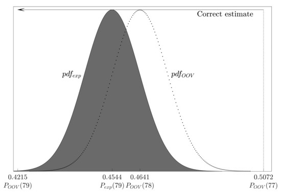
Figure 11.
The probability of an incorrect zero-bit guess when the weight estimate is incorrect: After flipping a zero-bit of a noise vector whose weight is optimal (=78), its acceptance rate follows the distribution ; nevertheless, after incorrectly estimating the weight of the vector as 77, the OOV algorithm estimates a bit as 0 iff
Since follows the distribution shown in Equation (13), the probability of an error, i.e., that the bit will be wrongly evaluated as 1, is:
Table 7 shows the probability that the OOV algorithm will wrongly estimate a zero-bit as a one-bit, when the noise vector weight is incorrectly estimated as 77. We can see how this probability changes as n increases. For each n we provide analytical value obtained from the Formula (20) as well as the value from the experimental results. The results demonstrate that the error made in the initial weight estimate can be neutralized during the bit guessing process and produce correct bit estimate.
Table 7.
Probability that the OOV algorithm will incorrectly estimate zero bit of the noise vector whose weight is incorrectly estimated as 77.
5.5. The Probability of an Incorrect One-Bit Guess when the Weight Estimate Is Incorrect
In the case when the observed bit is 1, after flipping it, the ratio follows the normal distribution (16). When the OOV algorithm incorrectly estimates the weight of the observed noise vector as 77, it will conclude that a bit is 1 iff (see Figure 12):
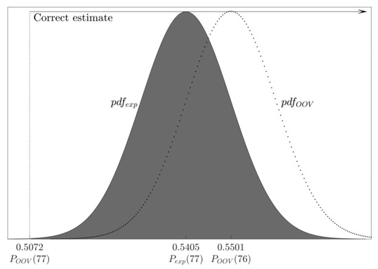
Figure 12.
The probability of an incorrect one-bit guess when the weight estimate is incorrect: After flipping a one-bit of a noise vector whose weight is optimal (=78), its acceptance rate follows the distribution ; nevertheless, after incorrectly estimating the weight of the vector as 77, the OOV algorithm estimates a bit as 1 iff .
Since follows the distribution (16), the probability of an error, i.e., that the bit will be wrongly evaluated as zero, is:
Table 8 shows the probability that the OOV algorithm will wrongly estimate a one-bit as a zero-bit, when the noise vector weight is incorrectly estimated as 77. We can see how this probability changes as increases. For each we provide analytical value obtained from the Formula (22) as well as the value from the experimental results. The results demonstrate that the error made in the initial weight estimate can be neutralized to some extent during the bit guessing process and produce correct bit estimate (the error rates are still somewhat higher than claim, for example, should limit the error to (see [13] and Section 5.6)).
Table 8.
Probability that the OOV algorithm will incorrectly estimate one-bit of the noise vector whose weight is incorrectly estimated as 77.
5.6. Key Recovery Probability
Previous analysis shows how the erroneous OOV Algorithm 1 for weight estimation, which uses the approximation that is not precise enough, can make two errors (the first one when estimating the weight of the original noise vector, and the second one when estimating its weight after flipping a bit), but the two errors can unintendedly cancel each other and output correct bit guess. Furthermore, the attacker can incorrectly estimate the weight, but correctly recover all the bits, and discover that the observed vector has one bit more than it is expected, having in mind the initial noise vector’s weight estimate. On the other hand, a greater problem occurs when the attacker correctly guesses the weight, and this happens with a probability that is not negligible. We will show that, practically, the only scenario in which the OOV attack can recover the key is the one in which weights are incorrectly estimated, but the errors mutually neutralize each other. Nevertheless, it will result in an increase of the necessary number of modifications , i.e., the overall complexity of the attack.
Based on the probabilities derived in Section 5.1, Section 5.2, Section 5.3, Section 5.4 and Section 5.5, we can calculate the probability of the successful recovery of a noise vector whose weight is optimal.
If the weight of a vector has been correctly estimated, the probability of success is:
For the parameter set II, this probability is equal for the HB# protocol, and for the Random-HB# protocol. On the other hand, if the weight of a vector has been incorrectly estimated as 77, the probability of correct bits recovery is:
For parameter set II, this probability is equal to 0.5949 for the HB# protocol, and 0.9802 for the Random-HB# protocol.
Since the probability that all bits of a noise vector, whose weight is optimal, will be correctly guessed after the weight has been estimated correctly is negligible, in order for the OOV attack to be successful, it is important that the optimal weight of this noise vector is estimated as (one) lower than its actual value. The OOV algorithm estimates the weight as 77 iff:
and:
Since follows the distribution , the probability that it falls into the interval is:
For the parameter set II, this probability is equal 0.9605 for the HB# protocol, and 0.9929 for the Random-HB# protocol. Let us notice that the probability that the weight of the noise vector whose weight is 78 will be estimated as something other than 77 or 78 is negligible.
In order to recover a key, an attacker needs 592 noise vectors in case of Random-HB# and four noise vectors in case of the HB# protocol. Hence, the probability an attacker will recover the key is equal in case of the Random-HB# protocol. In case of the HB# protocol, an attacker needs 1472 bits which correspond to three complete noise vectors and 149 bits of the fourth noise vector. The probability that 149 bits will be correctly estimated, when the weight is incorrectly estimated as 77 is:
where τ denotes the probability that a bit is 1, and for the parameter set II.
The probability (28) is equal 0.8818, and the probability the attacker will recover the key in the HB# protocol is .
Figure 13 and Figure 14 show how key recovery probability increases with an increase of the number of modifications and, consequently, the increase of the total (key recovery) complexity. In the OOV paper, for selected , which is equal 1382 for the HB# protocol and 2697 for the Random-HB# protocol, claimed error probability in the bit recovery process is . Thus, the error probability on a bit level is for HB# and for Random-HB#. At the same time, the error probability in the weight estimate process is equal . Based on this, we can derive that the claimed probability of a successful key recovery for the OOV algorithm is:
for HB# and:
for Random-HB#, which in both cases gives 0.37. However, as we have shown, due to the use of the approximation that is not precise (and fine) enough for this application, the actual probability is different and is equal 0.158 for HB# and for Random-HB#. The claimed precision can be achieved by increasing the number of modifications and, consequently, the total complexity of the key recovery algorithm. In case of the HB# protocol it is necessary to set to 1634 instead of 1382 (an increase of 18%). In case of the Random-HB# protocol it is necessary to set to 4196 instead of 2697 (an increase of 55%).
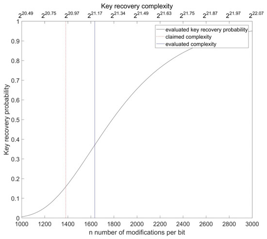
Figure 13.
The increase rate of the key recovery probability of the OOV algorithm for the HB# protocol depending on the number of modifications and total key recovery complexity. In order to achieve the attack precision claimed in [13], the number of modifications, i.e., the complexity of the attack, should be increased by 18%.
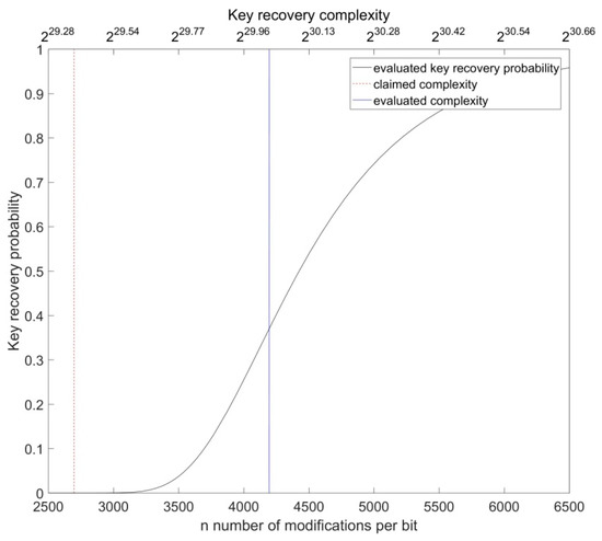
Figure 14.
The increase rate of the key recovery probability of the OOV algorithm for the Random-HB# protocol depending on the number of modifications and total key recovery complexity respectively. In order to achieve the attack precision claimed in [13], the number of per-bit modifications, i.e., the complexity of the attack, should be increased by 55%.
5.7. Loss of Precision with Block Optimization
The authors in [13] noted that the basic OOV algorithm (bit-by-bit recovery of the noise vector) can be optimized using an adaptive solution to the weighting problem [28]. Namely, instead of the approach where each bit of the noise vector is evaluated separately, the authors proposed an optimized algorithm which divides the vector into -bit windows and recovers the bits by measuring the weight using the following recursive procedure: (i) for each -bit window, estimate its weight, (ii) if the weight estimate is not equal either zero or the window size, split the window into two windows of the same length and measure each of them, taking into account the partial information obtained by the previous measurements. This leads to a lower number of measurements necessary to recover the noise vector, compared to the bit-by-bit algorithm. The authors examined the algorithm behavior for different window sizes and discovered that the optimal results (i.e., lowest complexity) is obtained for .
The non-optimized (bit-by-bit) version of the algorithm takes measurements in order to recover the noise vector of length , while the optimized (block-by-block) algorithm takes measurements, where is the average number of measurements needed to recover the bits in a -bit window. For the parameter set II, is equal 3.3585. The authors in [13] use the same number of modifications for both bit-by-bit and block-by-block version of the algorithm, and thus reduce the complexity of the optimized algorithm by the factor of in comparison to the non-optimized version.
Let us notice that in Algorithm 3 from [13] (the algorithm for finding errors in j-bit windows) at 8th line, the number of modifications used for estimating the weight of a sub-block is given with the factor 4, but there are two strong reasons to consider this as a slip in the pseudocode specification: (a) this is in contradiction with Formula (7) from [13] that gives the complexity of the OOV attack, and (b) if the complexity of the optimized algorithm was calculated with the factor 4, it would be higher than the complexity of the non-optimized algorithm.
The experiments we conducted showed that if the block-by-block algorithm uses the same number of modifications as the bit-by-bit version, the precision, i.e., key recover probability, decreases. Namely, for the HB# protocol and the parameter set II, the block-by-block algorithm for correctly recovered 122 keys out of 5000, which gives the precision of 0.0244, while the precision of the bit-by-bit version is 0.158.
These results can be explained by the following: when evaluating bits of a noise vector (whose weight is optimal), the bit-by-bit algorithm always decides if the weight of the vector changed to or after flipping the observed bit, while in the case of the block-by-block optimization, all the bits in the block are flipped together and the decision has to be made between multiple possible weights. For example, for a block of the size , after flipping eight bits, new weight of the observed noise vector is equal , where is the number of one-bits in that block. Since is unknown, the algorithm has to decide between the following nine possible weights: ,. However, in order to decide between, for example, weights and (in general, the weights that are further from the optimal), a number of modifications larger than the one for deciding between and has to be used in order to preserve the key recovery precision. This is not related to the quality of the acceptance rate approximation used in [13] and similar behavior should be noticed if the correct acceptance rate values are used.
6. Conclusions
The detailed evaluation and analysis presented in this paper provide additional insights on the OOV-MIM algorithm and these findings should be taken into account if the algorithm is employed in certain practical scenarios. The output of the core element of the OOV-MIM attack, Algorithm 1, depends on the approximation of the probability distributions which is shown to be not precise enough for this particular application. Due to this, Algorithm 1 gives erroneous results and, moreover, it cannot be corrected by increasing the “sample” size (number of interrupted authentication sessions). However, as a very interesting issue, this paper points out that the errors that result from Algorithm 1 can, unintendedly, cancel each other so that the resulting effect is not as “disastrous” as it could be. Nevertheless, this affects the total complexity of the attack.
An interesting issue for a future work would be to derive the exact probability distribution and find a better approximation to be used instead the one employed in [13]. Additionally, a challenge is the development of improved MIM attacks against the HB-class of authentication protocols.
Author Contributions
Conceptualization, M.K., S.T., and M.J.M.; formal analysis, M.K. and S.T.; funding acquisition, M.K., S.T., and M.J.M.; investigation, M.K.; methodology, M.K., S.T., and M.J.M.; software, M.K.; validation, M.K. and S.T.; writing—original draft, M.K., S.T., and M.J.M. All authors have read and agreed to the published version of the manuscript.
Funding
This research has been supported by the Ministry of education, science and technological development, Government of Serbia.
Acknowledgments
The authors thank the anonymous reviewers for their comments and observations which have provided guidelines for improvement of the paper results presentation.
Conflicts of Interest
The authors declare no conflict of interest.
References
- Avoine, G.; Carpent, X.; Hernandez-Castro, J. Pitfalls in ultralightweight authentication protocol designs. IEEE Trans. Mob. Comput. 2015, 15, 2317–2332. [Google Scholar] [CrossRef]
- Ibrahim, A.; Dalkılıc, G. Review of different classes of RFID authentication protocols. Wirel. Netw. 2019, 25, 961–974. [Google Scholar] [CrossRef]
- Baashirah, R.; Abuzneid, A. Survey on prominent RFID authentication protocols for passive tags. Sensors 2018, 18, 3584. [Google Scholar] [CrossRef] [PubMed]
- D’Arco, P. Ultralightweight cryptography. In International Conference on Security for Information Technology and Communications; Springer: Cham, Switzerland, 2018; pp. 1–16. [Google Scholar]
- Berlekamp, E.; McEliece, R.; Van Tilborg, H. On the inherent intractability of certain coding problems. IEEE Trans. Inf. Theory 1978, 24, 384–386. [Google Scholar] [CrossRef]
- Hopper, N.J.; Blum, M. Secure Human Identification Protocols. In Advances in Cryptology—ASIACRYPT 2001. ASIACRYPT 2001. Lecture Notes in Computer Science; Boyd, C., Ed.; Springer: Berlin/Heidelberg, Germany, 2001; Volume 2248. [Google Scholar]
- Katz, J.; Shin, J.S. Parallel and Concurrent Security of the HB and HB + Protocols. In Advances in Cryptology—EUROCRYPT 2006. EUROCRYPT 2006. Lecture Notes in Computer Science; Vaudenay, S., Ed.; Springer: Berlin/Heidelberg, Germany, 2006; Volume 4004. [Google Scholar]
- Katz, J.; Shin, J.S.; Smith, A. Parallel and concurrent security of the HB and HB+ protocols. J. Cryptol. 2010, 23, 402–421. [Google Scholar] [CrossRef]
- Gilbert, H.; Robshaw, M.; Sibert, H. Active attack against HB+: A provably secure lightweight authentication protocol. Electron. Lett. 2005, 41, 1169–1170. [Google Scholar] [CrossRef]
- Bringer, J.; Chabanne, H.; Dottax, E. HB++: A Lightweight Authentication Protocol Secure against Some Attacks. In Second International Workshop on Security, Privacy and Trust in Pervasive and Ubiquitous Computing (SecPerU’06); IEEE Computer Society: Washington, DC, USA, 2006; pp. 28–33. [Google Scholar]
- Munilla, J.; Peinado, A. HB-MP: A further step in the HB-family of lightweight authentication protocols. Comput. Netw. 2007, 51, 2262–2267. [Google Scholar] [CrossRef]
- Gilbert, H.; Robshaw, M.J.B.; Seurin, Y. HB#: Increasing the Security and Efficiency of HB+. In Advances in Cryptology—EUROCRYPT 2008. Lecture Notes in Computer Science; Smart, N., Ed.; Springer: Berlin/Heidelberg, Germany, 2008; Volume 4965. [Google Scholar]
- Ouafi, K.; Overbeck, R.; Vaudenay, S. On the Security of HB# against a Man-in-the-Middle Attack. In Advances in Cryptology—ASIACRYPT 2008. Lecture Notes in Computer Science; Pieprzyk, J., Ed.; Springer: Berlin/Heidelberg, Germany, 2008; Volume 5350. [Google Scholar]
- Rizomiliotis, P. HB−MAC: Improving the Random−HB# authentication protocol. In International Conference on Trust, Privacy and Security in Digital Business; Springer: Berlin/Heidelberg, Germany, 2009; pp. 159–168. [Google Scholar]
- Leng, X.; Mayes, K.; Markantonakis, K. HB-MP+ protocol: An improvement on the HB-MP protocol. In 2008 IEEE International Conference on RFID; IEEE: Piscataway, NJ, USA, 2008; pp. 118–124. [Google Scholar]
- Yoon, B.; Sung, M.Y.; Yeon, S.; Oh, H.S.; Kwon, Y.; Kim, C.; Kim, K.H. HB-MP++ protocol: An ultra light-weight authentication protocol for RFID system. In 2009 IEEE International Conference on RFID; IEEE Computer Society: Washington, DC, USA, 2009; pp. 186–191. [Google Scholar]
- Aseeri, A.; Bamasak, O. HB-MP*: Towards a Man-in-the-Middle-Resistant Protocol of HB Family. In 2nd Mosharaka International Conference on Mobile Computing and Wireless Communications (MIC-MCWC 2011); Mosharaka for Research and Studies: Amman, Jordan, 2011; Volume 2, pp. 49–53. [Google Scholar]
- Bringer, J.; Chabanne, H. Trusted-HB: A low-cost version of HB+ secure against man-in-the-middle attacks. IEEE Trans. Inf. Theory 2008, 54, 4339–4342. [Google Scholar] [CrossRef]
- Madhavan, M.; Thangaraj, A.; Sankarasubramanian, Y.; Viswanathan, K. NLHB: A non-linear Hopper-Blum protocol. In 2010 IEEE International Symposium on Information Theory; IEEE: Piscataway, NJ, USA, 2010; pp. 2498–2502. [Google Scholar]
- Bosley, C.; Haralambiev, K.; Nicolosi, A. HBN: An HB-like protocol secure against man-in-the-middle attacks. IACR Cryptol. ePrint Arch. 2011, 2011, 350. [Google Scholar]
- Rizomiliotis, P.; Gritzalis, S. GHB#: A provably secure HB-like lightweight authentication protocol. In International Conference on Applied Cryptography and Network Security; Springer: Berlin/Heidelberg, Germany, 2012; pp. 489–506. [Google Scholar]
- Hammouri, G.; Öztürk, E.; Birand, B.; Sunar, B. Unclonable lightweight authentication scheme. In International Conference on Information and Communications Security; Springer: Berlin/Heidelberg, Germany, 2008; pp. 33–48. [Google Scholar]
- Hammouri, G.; Sunar, B. PUF-HB: A tamper-resilient HB based authentication protocol. In International Conference on Applied Cryptography and Network Security; Springer: Berlin/Heidelberg, Germany, 2008; pp. 346–365. [Google Scholar]
- Deng, G.; Li, H.; Zhang, Y.; Wang, J. Tree-LSHB+: An LPN-based lightweight mutual authentication RFID protocol. Wirel. Pers. Commun. 2013, 72, 159–174. [Google Scholar] [CrossRef]
- Qian, X.; Liu, X.; Yang, S.; Zuo, C. Security and privacy analysis of tree-LSHB+ protocol. Wirel. Pers. Commun. 2014, 77, 3125–3314. [Google Scholar] [CrossRef]
- Tomović, S.; Mihaljević, M.J.; Perović, A.; Ognjanović, Z. A Protocol for Provably Secure Authentication of a Tiny Entity to a High Performance Computing One. Math. Probl. Eng. 2016, 2016, 1–9. [Google Scholar] [CrossRef]
- Tomović, S.; Knežević, M.; Mihaljević, M.J.; Perović, A.; Ognjanović, Z. Security evaluation of NHB# authentication protocol against a MIM attack. IPSI BgD Trans. Internet Res. (TIR) 2016, 12, 22–36. [Google Scholar]
- Erdos, P.; Rényi, A. On two problems of information theory. Magyar Tud. Akad. Mat. Kutató Int. Közl 1963, 8, 229–243. [Google Scholar]
© 2020 by the authors. Licensee MDPI, Basel, Switzerland. This article is an open access article distributed under the terms and conditions of the Creative Commons Attribution (CC BY) license (http://creativecommons.org/licenses/by/4.0/).