1. Introduction
The world’s urban population has tended to increase at the expense of migration from rural areas [
1], with the current urban population being approximately 55.7% of the world’s population [
2]. Furthermore, predictions say that by 2030, 60.4% of the world’s population will be living in urban areas and will be concentrated in the most developed countries, where they will represent 81.4% of the population [
3]. Therefore, large human concentrations will be present in megacities, which must be planned so that they can provide their services intelligently and efficiently. Usually, these services are based on the deployment of systems, mainly wireless systems (e.g., Internet-of-Things (IoT), 5G, and Wireless Sensor Networks (WSN)) [
4], because these systems can connect mobile users at any time and any point inside a megacity.
Therefore, the implementation of a smart city (SC) is necessary, requiring the cooperation of cities and city authorities, investors and funding agencies, researchers, and citizens [
5]. In this context, SCs must be designed as megacity projects focused on a technologically structured perspective [
6]. Because the demand for spaces and services is high, the construction of very tall buildings, such as so-called skyscrapers, is necessary. The technological development of those buildings includes the incorporation of intelligence (e.g., smart buildings (SBs)) so that they can provide services efficiently, considering horizontal and vertical integration models in the building inside [
6].
For successful improvements in the services provided, building users prefer wireless communication technologies over wired networks. The building communication service providers prefer to use inner short-range systems (e.g., Internet-of-Things (IoT) technology), since they are straightforward to deploy while, at the same time, offering flexibility, portability, and scalability [
7]. This means that inside SBs located in an SC, many short-range systems will be operating and providing mobile services to their users (e.g., Bluetooth, Wi-Fi, Long-Term Evolution (LTE)/ Global System for Mobile communications (GSM) femtocells, Wireless Sensor Networks (WSN), ZigBee, and Radio-Frequency Identification (RFID)) [
8].
These futuristic scenarios are rapidly developing throughout the world. A forecast announced that by 2022, the increase in wireless connectivity would bring wireless traffic close to 84% of the total Internet traffic and the total amount of Internet traffic would be approximately 11 times the mobile traffic generated in 2017 [
4]. As a result, there could be a high quantity of connected devices that increase wireless traffic. This could lead to interference, especially if they work in the same frequencies (e.g., the Industrial, Scientific and Medical (ISM) Band).
There are at least two ways to avoid interference due to spectrum congestion; one of them is requiring new frequency bands, and the other is dynamically reusing the spectrum of any incumbent operator (i.e., Dynamic Spectrum Access (DSA)) to improve the current efficiency in the use of the spectrum [
9]. This last method requires the spectrum to be managed on a DSA basis [
10] instead of using the traditional Command and Control [
11] model.
The changing trend in spectrum management is based on some studies showing that the spectrum segments assigned to wireless telecommunication service operators have relatively low average use in both rural and urban areas [
11,
12]. In other words, these studies have proved that there is spatial and temporary availability of the licensed spectrum, which could be used dynamically for the same or different services provided by the incumbent operators themselves or by a new operator [
10].
DSA means that a non-licensed system can use an available segment from the spectrum assigned to incumbent operators in any spatial position without causing interference to incumbent users; in this context, the incumbent operator is called the Primary System (PS), while the operator that makes dynamic use of the spectrum is called the Secondary System (SS) [
13]. Here, it is crucial to indicate that Cognitive Radio (CR) is a wireless system that uses the DSA to make efficient use of the spectrum [
13], so CR-based systems can act like an SS.
Wireless systems based on CR have the functionality of intelligently changing their transmission/reception parameters to try to maintain continuity in the service, despite using the time-changing spectrum availability of the spectrum segment of the primary band [
14]. For its operation, an SS based on CR must perform the process of finding spectrum availability in the PS; then, this spectrum information is passed through a set of policies to obtain an effective spectrum availability (ESA) that can be used opportunistically and intelligently [
14]. Therefore, for the operation of CR systems within an SB, it is necessary to identify and quantify the ESA.
To find the available spectrum segments, different strategies can be used, which are consolidated into two broad groups: one of them using information provided by specialized databases and the other using local measurements [
10]. However, by using the information of the databases or by using internal spectrum measurements, the internal spectrum availability information would only indicate the presence of white space, i.e., it indicates either the presence or absence of the incumbent operator. For example, determining the building’s inner white spaces on the TV band known as TV white space (TVWS) does not guarantee that a non-licensed operator can effectively use the building’s internal available spectrum because they could cause interference to primary users.
Indoor TVWS and ESA are similar but not the same because the TVWS is found using the power level measurements of the Primary Band and a threshold level, while ESA determination requires that when the SS transmits using the TVWS, it does not interfere with the building TV receiver device’s internal deployment. Thus, for obtaining the ESA, it is necessary to consider an additional condition, the minimization of the possible local interference that CR-based short-range wireless systems (SR-CRWS) could produce on the incumbent user network deployed inside the SB [
10,
15]. Because CR must work with reusable available spectrum, the ESA determination inside a building has become a real and current challenge.
Moreover, determining the ESA would have the benefit of allowing the operation of a private wireless service or system that could be planned in the interior of an SB without the need to use new spectrum bands. Such interior systems could be SR_CRWS, such as cognitive wireless networks and cognitive wireless home networks, using any current technology (e.g., Wi-Fi, GSM, or LTE) [
9].
Since the SSs proposed here will operate inside buildings, they need to use a frequency segment that can quickly propagate through internal walls. That is, a spectrum that can overcome inner obstacles using low transmission power levels is required—obstacles such as the interior walls of a building, for example. The band assigned to TV broadcast fulfills such requirements [
16,
17]. This work uses TVWS for efficient spectrum reuse because it allows broadband connectivity and IoT connectivity, providing solutions for private networks, smart grids, and smart buildings, among others [
18]. Nevertheless, it is very important to clarify that this procedure can be replicated for the other primary bands.
Considering that, this article proposes a validated measuring mechanism that allows the estimation of the lower available amount of ESA inside an SB located in a smart city dense urban area with an appropriate inner deployment of incumbent users.
2. Related Work
Obtaining effective TVWS, both outside and inside buildings, is a growing concern, so new studies are trying to improve the information on TVWS geolocated databases or to complement the process of indoor spectrum measurements.
A study tried to find an effective TVWS to enable a low-cost, last–middle-mile access infrastructure for rural regions [
17]. It found that the effective available TVWS quantity in rural regions can be lower than the TVWS quantity reported by geolocated databases. This may be due to the interference toward the primary users. Another study [
19] tried to deploy an LTE stand-alone system working in the 5 GHz unlicensed spectrum that shares the spectrum with Wi-Fi devices. The simulations showed that the stand-alone LTE system can provide more capacity and coverage than the Wi-Fi network.
In Verulam, South Africa, a comparative study [
20] was carried out of the TVWSs measured and those predicted by a geolocated spectrum database. The results show that, in sites with a physical blockage, the difference between compared values can be very large. For this reason, this study suggests that, for greater precision, the TVWS geolocated-database information should be compensated for with real-time measurements.
For the case of spectrum availability inside a building, a study [
21] proposed a model to estimate a TVWS link budget. That model uses internal measurements in a few sites inside a building and compares them with other models and obtains good results in terms of the root-mean-square error. Another indoor study proposed a hybrid system that combines Broadband Power Line Communication (BPLC) and a TVWS CR system to improve the system capacity; interference was mitigated with an iterative precoding algorithm [
22].
Additionally, an experimental study determined both the behavior and a statistical model of the spectrum availability to find the joint availability of the channels of several TV incumbent operators inside a building in Guayaquil city, Ecuador, to quantify the nominal capacity that could be available for use by the SSs based on the CR [
15]. Another two studies used the ESA concept, the first one [
23] using it to characterize the available spectrum opportunities inside buildings and showing that the SR-CRWS could operate like the SS there, and the other one [
24] focusing on discovering the effects of shadowing phenomena on the spectrum availability in building interiors.
Unlike the studies presented, this study aimed to estimate and quantify the ESA inside an SB using three known propagation models to validate the outdoor path loss component. The propagation models used in this proposed mechanism were validated using two measurement campaigns carried out inside two buildings located in the urban area of the city of Guayaquil, Ecuador. This study used TV band frequencies for their propagation properties inside buildings.
3. System Model
This section describes the proposed scenario for ESA estimation, the interference conditions model, the ESA estimation model, and the used metrics.
3.1. Scenario Description
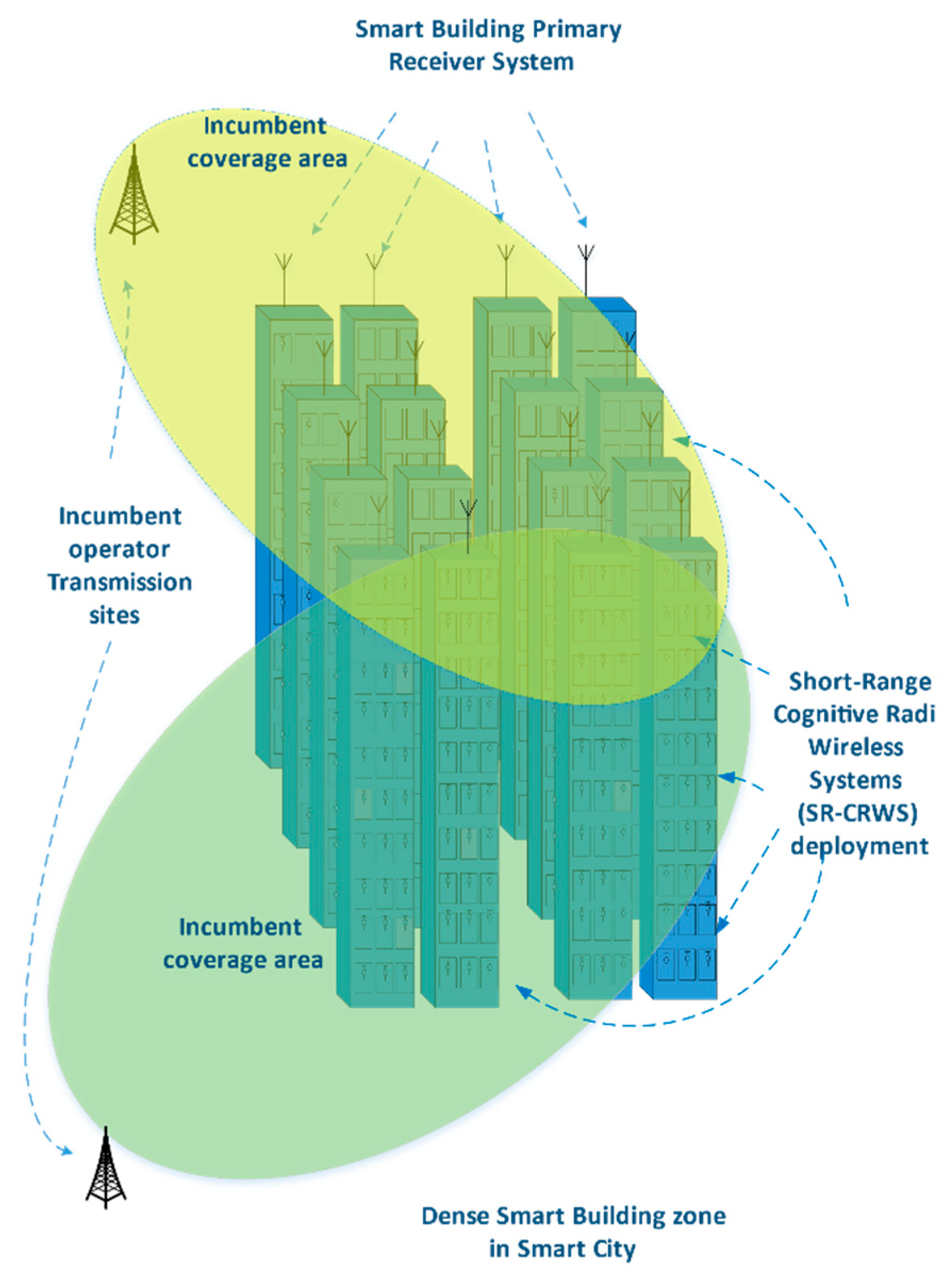
Figure 1 shows a dense urban area with highly homogeneous buildings, which maintain a high demand for internal wireless communication services (e.g., an SB) and being part of a megacity (e.g., an SC), shaping a scenario that looks like a Manhattan grid. In the same
Figure 1, all the SBs are within the incumbent coverage area, which is radiated by robust systems (e.g., broadcast TV systems); the incumbent operators are the PS.
Inside every SB, all apartments get allocated one SR-CRWS that can operate like an SS. All SR-CRWS have their own operation frequencies (e.g., ISM bands), but under strong interference conditions, they use the available inner spectrum to maintain the service. Likewise, the deployment of primary users (PUs) is considered, and this is represented by an antenna located on the rooftop of the building. It is important to note that the said antenna feeds an internal distribution system, not shown in the figure, which uses a wired network (i.e., coaxial cable). As a result, the deployment of the PUs occurs when the antenna on the rooftop of the building senses interferences.
Although it is common for the different SBs in an SC to be heterogeneous, in this study, the internal distribution in the SBs was identical, such that each building had N apartments of equal dimensions. Therefore, on each floor, the same number of SR-CRWSs was deployed to allow the opportunistic use of the PS spectrum if required.
To determine the lower amount of spectrum availability inside the building, this study was performed in an SB that received the maximum power level of the PS. This building had one face receiving wave propagation at a normal incidence position; also, it needed a line of sight (LOS) from all its floors to the base station (BS). Finally, the effects of the power level reflected from neighboring buildings were considered. The scenario was conveniently adjusted to achieve the most restrictive spectral availability conditions for obtaining the ESA.
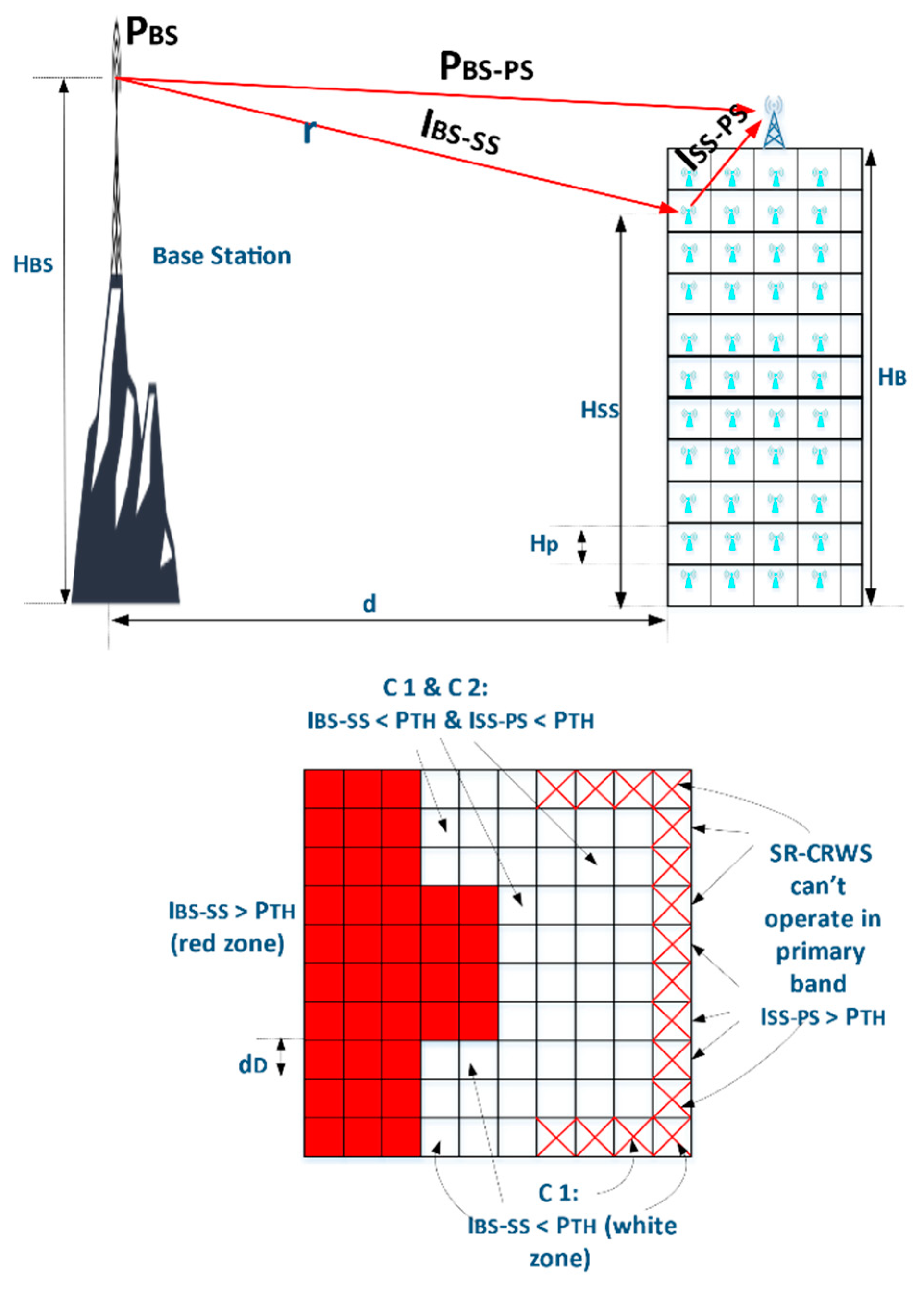
As shown in
Figure 2, a BS of a primary system was located at a distance d opposite to the face of an SB with dimensions
. The BS had an antenna with a height
that radiated the power
using the operating frequency
f, while the SB had a height
, where p represents the number of floors of the building and
represents the height of each story.
Additionally,
Figure 2 shows a floor of the building where three regions stand out: red apartments, white apartments, and white apartments with red stripes. The white apartments indicate the inner SB area where there is effective availability of a primary band, contrary to the red apartments, which represent apartments without spectrum availability, and the white apartments marked with red stripes represent the zone where an SS producing interference with the PS is located.
The white apartments represent the zone where the SS can use the spectrum available. This last zone represents the ESA for each floor, the zone where the spectrum can be used for CR-based systems.
3.2. Interference Conditions Model
Based on this scenario, the two interference conditions necessary to estimate the ESA are explained; the first condition determines the use of the incumbent spectrum, and the second checks whether interferences are produced toward the deployment of primary band users inside the building.
The first condition is called Condition 1 (C1), and its purpose is to establish the absence or presence of the PS. C1 allows the identification of the apartments where the interference received in the SS from the BS would not be at a sufficient level to overcome a reference level . It should be clarified that was called interference because the SS was operating in its own band (e.g., the ISM band), and any other received signals were considered interference. The reference power level used in this work was the sensitivity of a digital terrestrial television receiver.
Since the determination of C1 involves both an external path from the BS to the SB with a LOS and an internal route inside the SB, several propagation models were evaluated for use. For the case of the interior path, the model of the penetration of buildings without a line of sight (NLOS) was evaluated, and for the LOS component, unlike in [
23,
24], three known propagation models were evaluated: the Free Space Model (FRIIS) [
25], the Egli Propagation Model (EGLI) [
26], and the LOS component of the COST 231 Walfisch–Ikegami (COST-WI) Model [
25]. The FRIIS model was considered because it is a good indicator of path losses, the EGLI model was used because it considers wave propagation on uneven terrain, and the LOS component of COST-WI was considered because is a widely used reference; thus, in this work, the propagation model with the best correlation factor concerning two measurement campaign results was chosen.
The second condition, called Condition 2 (C2), allows the determination of the apartments from which an SR-CRWS would not cause interference to the PS receiver located on the rooftop of the building. For this condition to be met, the interference level
could not exceed the minimum threshold level supported by the PS receiver; the threshold level, as in C1, was the sensitivity of a TV receiver. Consequently, both C1 and C2 are described as follows [
24]:
To calculate C2, the Multi-Wall Model (MWM) [
25] was used to evaluate the measurement above the campaign. The apartments where C1 and C2 were true made up the region with the ESA.
3.3. C1 Model
The propagation losses between the BS and the place where each SS was located can be determined using the penetration loss with the NLOS conditions model [
25] as follows:
represents the LOS model component and is the propagation loss between the transmitting antenna and the incident wall, while represents the internal path propagation loss of the SB. is the attenuation from the building’s external wall, and compensates for the penetration of the outer walls. is the total loss considering interior walls, represents the total ascending loss, and is a measure of the total gain due to the height of the SS, using the floor gain in dB/floor with floors or the height gain in dB/m with height .
According to the FRIIS model,
can be represented by [
25]
where
is the operating frequency in MHz, and
is the path length in km.
When considering the EGLI model,
is represented by the following expression [
26]:
where
is the height in meters of the antenna of the primary system and
is the height in meters of the measuring point.
The third model considered, the COST-WI LOS component, is represented in
by the following equation [
25]:
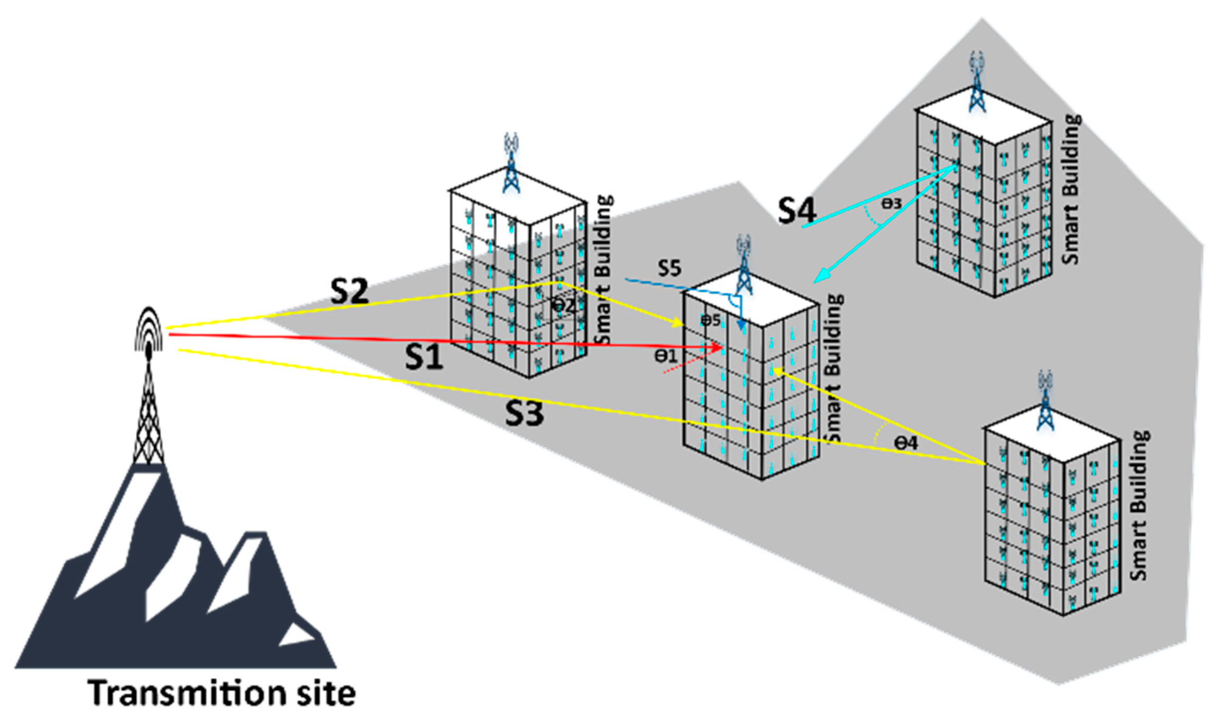
To model the power level with a high level of precision, the power contribution of the surrounding SBs inside an SC was considered. For this reason, a five-ray model was used: three reflected rays corresponded to reflections due to neighboring buildings, and the two other direct rays came from the BS, as shown in
Figure 3. The angles shown in the figure were used to find the appropriate power level in the specific direction of both the incident rays and reflected rays. All the power contributions were added to minimize the spectrum availability inside the SB.
The first four rays were calculated as horizontal components of the power level received from the transmission site, and the fifth ray was the vertical component of the incident power that crossed the roof of the building. Therefore, by replacing it in Equation (1), we found that Condition 1 was satisfied if
where
represents the path of the BS signal on each of the four faces and the roof of the building, and
is the factor that corrects the direction of the path for the normal incidence of each ray.
3.4. C2 Model
Recalling the definition established in Equation (2), we have an apartment that meets C2 when
where
corresponds to the loss of propagation using the MWM [
25] between the SR-CRWS and the PS receiver located on the rooftop of the building.
is the power emitted from the SR-CRWS. The MWM is represented by
The MWM model considers a free space loss
between the PS receiver of the building and the SS, while the
constant is a parameter that is used to compensate losses, which are usually negligible;
represents the losses in each internal wall, the number of walls of
type that cross the inner path is
,
represents the slab loss, and
represents the number of slabs that are traversed and is complemented by an empirical factor
. Therefore, Condition 2 is satisfied if
3.5. Effective Spectrum Availability Model
The ESA uses a metric that represents the percentage of the internal area of the building in which the primary spectrum can be reused. It is obtained from the ratio between the number of apartments within an SB from where an SR-CRWS can operate as an SS and the quantity of building apartments.
The ESA estimation mechanism proposed is based on the simultaneous fulfillment of the two interference conditions in each apartment of the SB; to estimate the ESA on each SB floor
, both C1 and C2 must determine the apartments that meet both conditions at the same time. To identify these apartments on each floor
, they are assigned binary values as follows:
Once the apartments have been correctly identified, they are grouped by floor to determine the
, as shown below:
Finally, the ESA is determined using
In other words,
and finally,
where the LOS component
is evaluated and validated in the next section.
4. Interference Model Validation
In this section, the two scenarios used in the measurement campaign for the power levels and the results of the interference condition validation are presented.
4.1. Measurement Scenarios
To evaluate the propagation models proposed in
Section 3, two power level measurement campaigns were carried out inside two different buildings in the urban downtown area of the city of Guayaquil. To validate the propagation model for the lowest floors, a small building with four floors and a rooftop was used, and to validate it for the upper floors, a 25-story building was utilized.
The small building was located at the coordinates −2.220144°, −79.888879° and had a height of 16 m (). The Radiofrequency (RF) broadcast was made from a simulated BS from a nearby building. This scenario was used to evaluate the three propagation models in the lower floors and determine among them the one to be considered for the calculation of the path loss external component in the subsequent simulations.
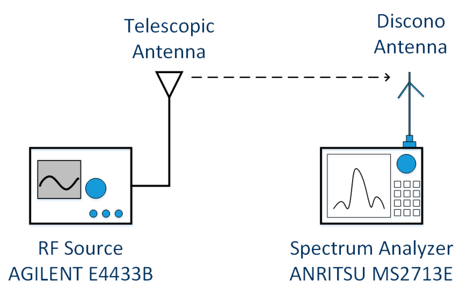
The transmission system used is shown in
Figure 4. It consisted of an RF generator (Agilent model E4433B) emitting +20 dBm of power (
), a generic omnidirectional unity gain antenna with a height of 23.4 m (
) that was installed on the rooftop located close to the target building at a distance of exactly 16.5 m (
). The receiving system was located inside the target building and used a portable spectrum analyzer (Anritsu model MS2713E) and a Discono SIRIO 2000 multiband antenna. The operating frequency of the system was 635 MHz (
), radiating a frequency modulated (FM) carrier with a bandwidth of 1 MHz.
To define the external component in the path loss propagation model to be used in subsequent simulations, the power levels were measured at the midpoints of three apartments located in front of the BS for each floor of the building. Additionally, for the building inner level power measurements, other measurements were taken at the central point of the building’s rooftop, but this time, power was transmitted with the RF source from inside the building simulating an SR-CRWS for the purpose of validating the MWM model.
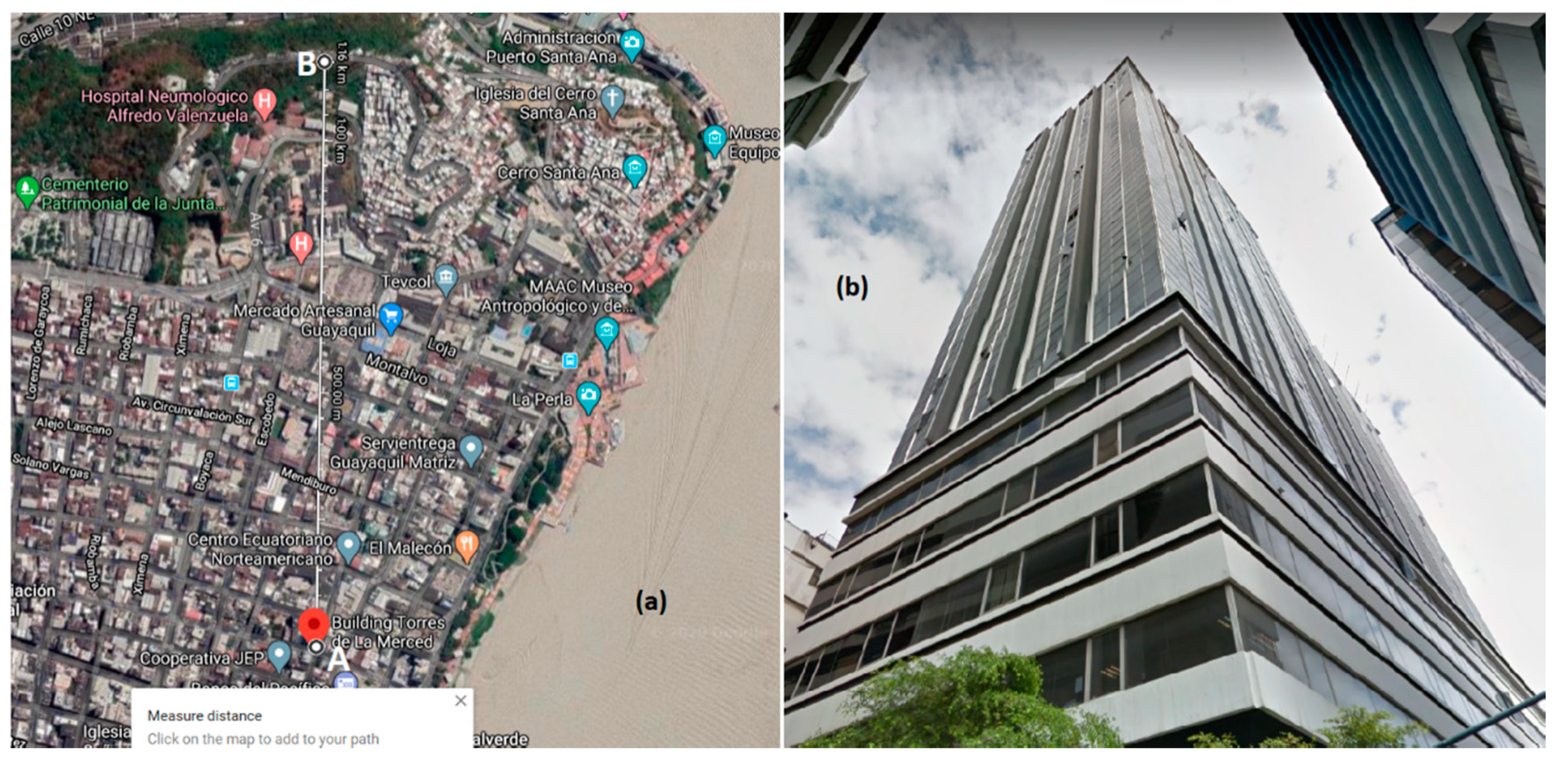
On the other hand, the validation of the propagation models for the upper floors used the campaign results for the power levels of a TV channel in a 25-story building. The building Torres de la Merced is located at the coordinates −2.1903656, −79.8834593, as can be seen in
Figure 5. The power levels of the 25 Ultra High Frequency (UHF) TV channel were measured for one hour at the same place within each floor using a spectrum analyzer (ANRITSU model MS2713E).
The BS of channel 25 UHF was in the Cerro del Carmen at an approximate height of 50 m above sea level, while the radiating elements were located on a 60 m structure above the previous reference. As can be seen in
Figure 5a, the BS (point B) was separated from the Torres de la Merced (point A) by approximately 1.16 km. It is important to note that this large building had a 16-story tower attached at one side with a LOS to the BS, as shown in
Figure 5b.
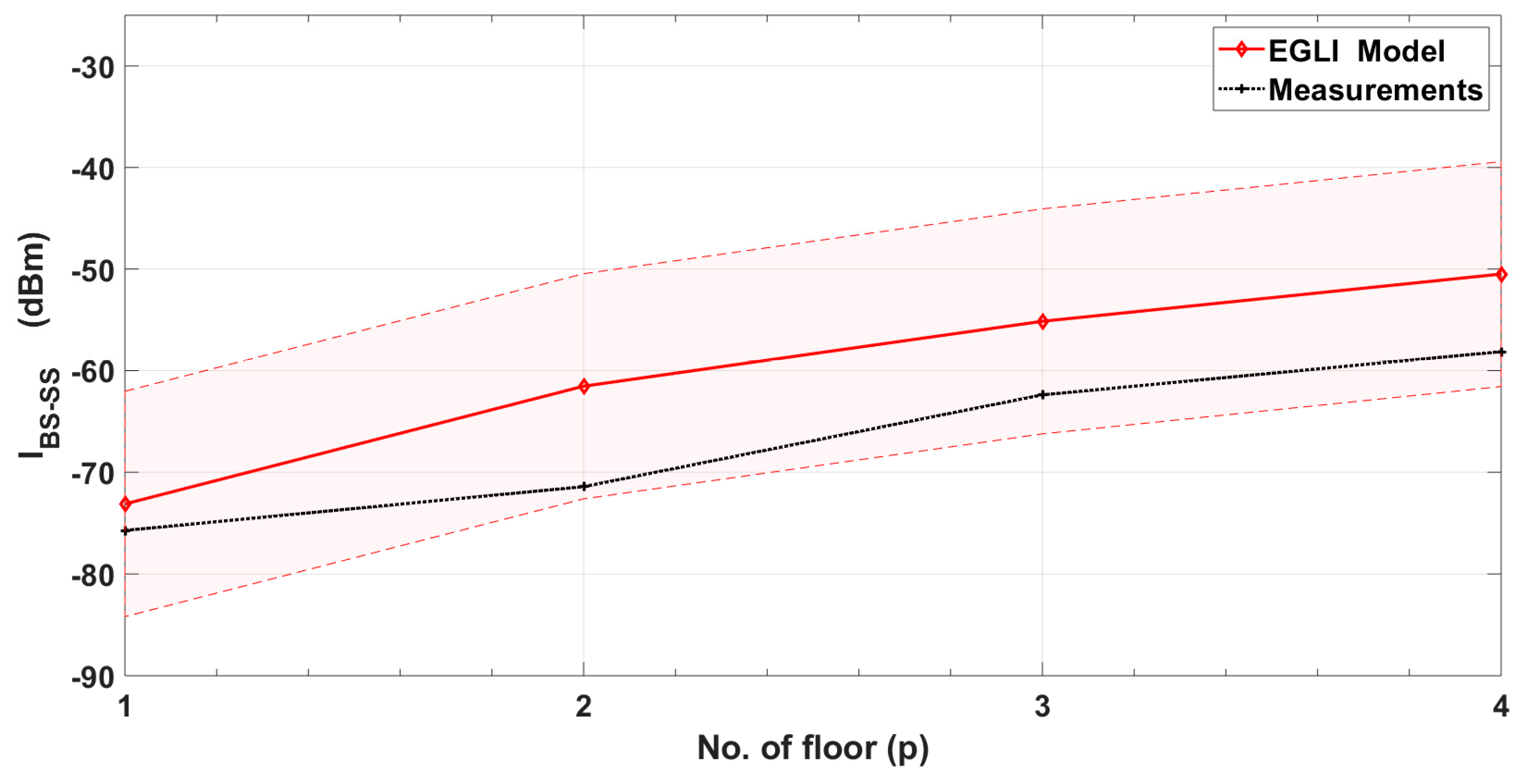
4.2. C1 Interference Condition Model Validation
Then, we proceeded to validate the propagation models used to determine the interference condition C1. The power levels obtained from both scenarios—a short building and a tall building—were used separately for C1 validation by comparing these results with the power levels that would be obtained using each of the three propagation models. The three outdoor propagation models proposed were used to evaluate the
values, as explained in
Section 3.
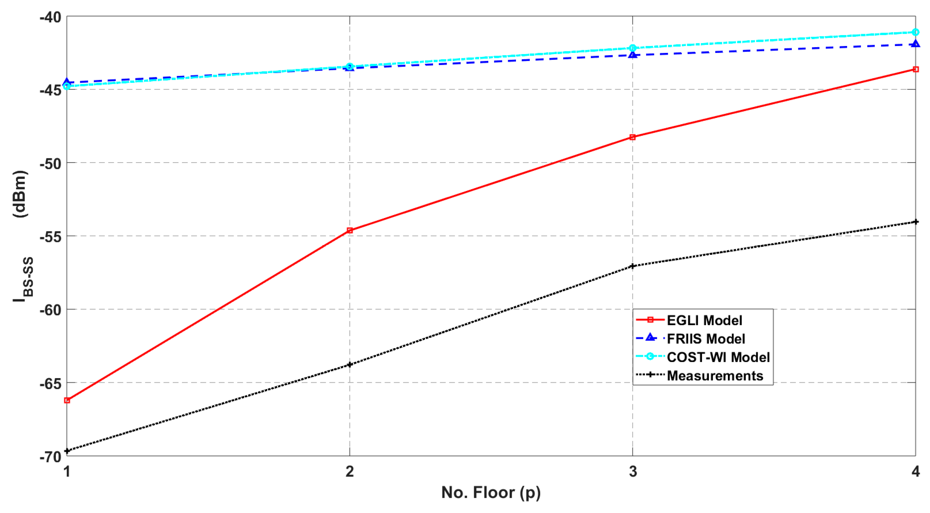
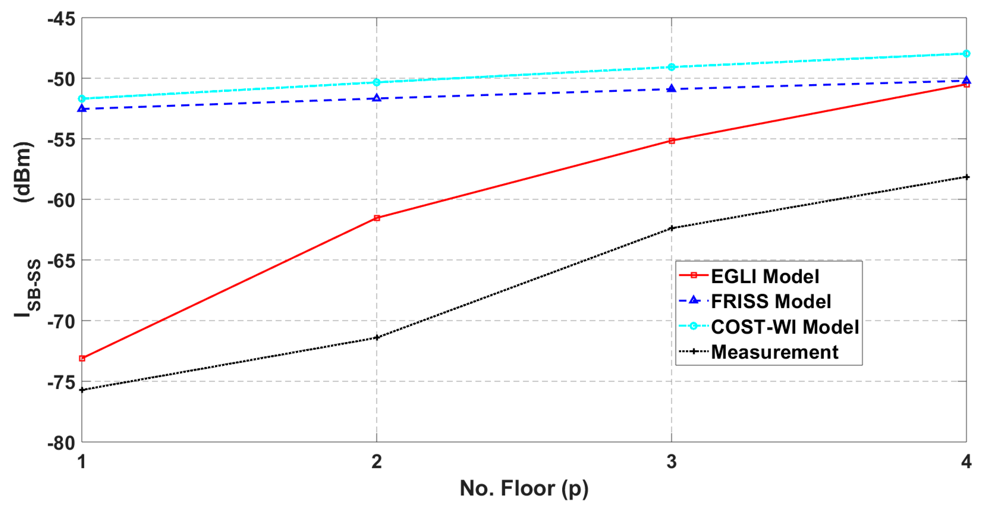
In the case of the small building, the comparisons of the measured and simulated power values are shown in
Figure 6 and
Figure 7, where the values of the interference
can be appreciated. In those figures, the FRIIS model is represented by the blue line; the COST-WI model, by the cyan line; and the EGLI model, by the red line, and the black line represents the measured power levels.
As expected,
Figure 6 and
Figure 7 show that the front apartments received higher levels of interference than the apartments located in the middle of the building or at the back of it. Additionally, the interference levels increased with height, which is predictable since as the height of the measurement point increased, the receiver device further approached the broadcast site, according to the scenario proposed.
Additionally, it was observed that the EGLI propagation model best approximated the interference levels measured. On the contrary, the WI and FRIIS models presented significant variation in the interference level on the lower floors of the building, because they did not consider heights for their determination. However, the three propagation models tended to exhibit similar behavior when the height of the floors approached the height of the SB antenna.
Moreover, the interference levels from the measurement campaign were lower than those simulated. This was due to the characteristics of the proposed scenario, because the simulation did not account for all of the real stationary obstacles, such as furniture, or those in motion, such as people inside the building.
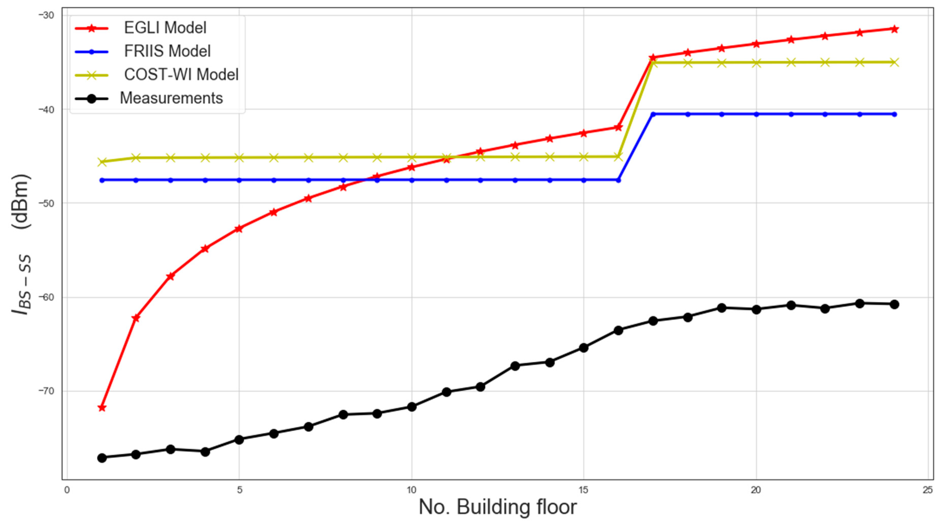
For the tall building, the power values measured inside the building and the values simulated by the three propagation models under study are compared in
Figure 8.
In
Figure 8, the power values found by simulation varied sharply on the 16th floor, because the obstruction of the attached building was considered. The behavior simulated using the FRIIS and COST-WI models showed quasi-constant values in the two sections of the building, while the EGLI model showed increasing behavior. It can be verified that, as in the small building, the behavior of the EGLI model was more adequate than that of the other models in the sector containing the lower floors.
To establish the best-simulated behavior, an analysis of the correlation coefficients of the measurements was performed for each of the models under study.
Table 1 shows the values of the correlation coefficients, where it can be seen that all of the simulated propagation models correlate quite well with the measurements made.
Table 1 shows that the propagation model with the highest correlation coefficient is the EGLI. For this reason, and in line with the proposed objectives, for the remainder of this study, only the EGLI model was considered for the
component in the implementation of C1.
4.3. Influence of Shadowing Phenomena
During a measurement campaign, the instantaneous values vary very quickly, so the influence of shadowing phenomena on the average measured value and the simulated value should be considered.
Considering that the values obtained with a propagation model are average values and because shadowing is a random process, the simulated values can vary within a range. The range is variable, so it is customary to represent it with a parameter called the confidence interval (CI).
The standard deviation of a propagation model
due to shadowing can be determined from the following expression for the case of macro-cells [
27]:
The value of the losses by shadowing
is found using
where
t is the probability of being within the coverage of the macrocell,
.
where
Q (
t) is the tail distribution function of the normal distribution. Due to shadowing, the received power may be higher or lower than the power value calculated by a propagation model; thus, the upper and lower limits of the power values obtained by simulation define a CI for the measured interference values with a probability
.
Figure 9 shows a shaded area above and below the red line. This area indicates the probable zone of the interference levels of the EGLI model considering a probability of CI = 0.95, compared with the measurements made in the central apartment of the building. The graph shows that all the values obtained in the measurement campaign were entirely within the CI given by the simulation values.
The shadowing phenomena are multiplicative noise in the communication channel, where additive noises such as white noise and thermal noise also intervene. The power levels of the additive noise can influence to a greater or lesser extent the power level of the received signal. The white noise levels depend directly on the electromagnetic pollution of the study environment, while the level of noise produced in a receiver due to thermal noise can be calculated, considering a temperature of 27 °C, according to [
27]:
where
is the channel bandwidth in Hz and
is the device noise figure in dB.
Considering a 6 MHz bandwidth TV channel and a TV receiver with an average noise figure of 8 dB; using (22), a total noise of −98 dBm is obtained in the receiver, which gives a margin of 23 dB with respect to the threshold level; this margin would also allow controlling the variations in the power level due to white noise. For these reasons, this study does not include a detailed study on the influence of additive noises since they present power levels much lower than the threshold power level.
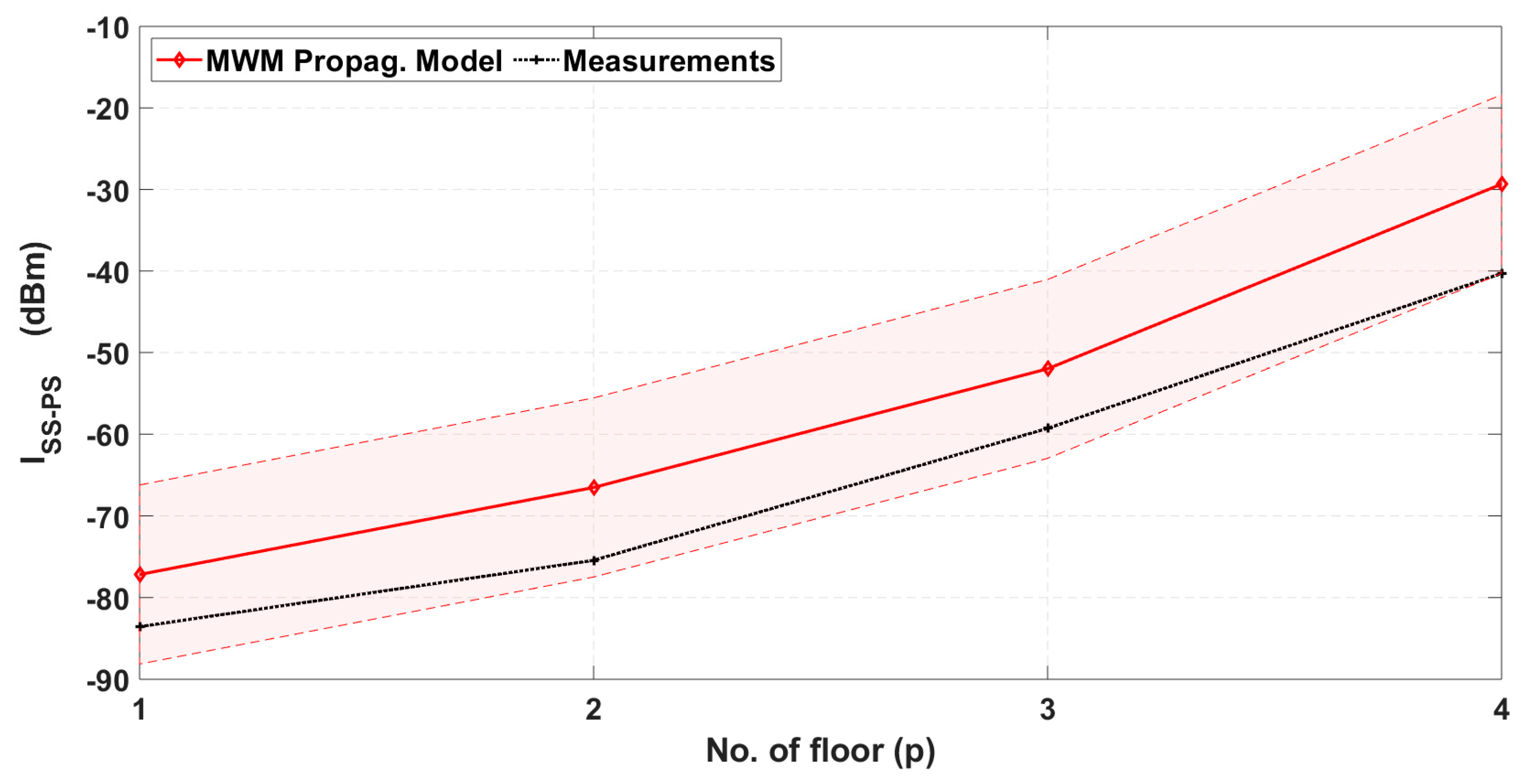
4.4. C2 Interference Condition Model Validation
As for the previous case, we validated the behavior of the MWM model used by C2 to determine the possible interference on the reception system of the primary service located on the rooftop of the building. This check was only performed in the small building.
It should be emphasized that, for the measurement of the interference, we used the receiver system installed in the middle sector of the rooftop and the transmitter system operated from the central position of each floor of the small building.
A comparison of the measured values (black line) against the values obtained in the simulation with the MWM model (red line) is shown in
Figure 10. The dashed red lines show the maximum and minimum limits of the CI = 95% due to shadowing. The figure shows that the behavior of the values of the model was similar and that all the values of the measurements were within the limits of the CIs. Finally, since the correlation between the measured and simulated data was calculated and found to be 0.987, the C2 interference model was fully validated using the MWM model.
5. ESA Model Performance
Once the propagation models with the measurement campaigns inside the buildings had been validated, both the EGLI model for the outdoor path in the C1 interference model and the MWM model in the C2 interference model were set up under the conditions outlined in
Section 3 to implement the mechanism for obtaining the ESA. In this section, the analysis of the ESA mechanism’s performance is performed using the parameters shown in
Table 2. The first analysis of the results refers to the ESA per floor (ESAF), and then an analysis was performed for the entire SB to obtain the ESA.
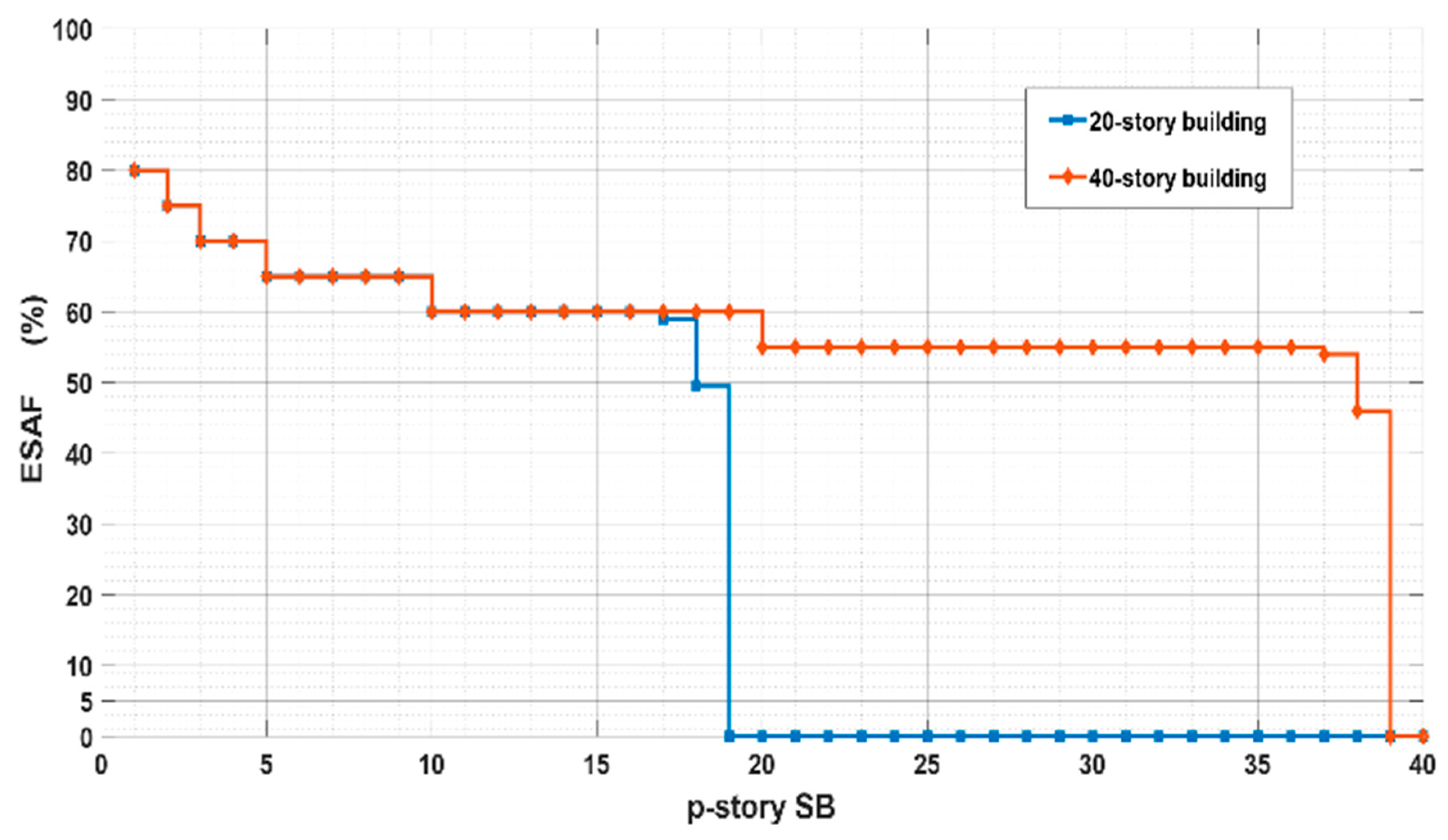
The ESAF behavior for two SBs is shown in
Figure 11. The results indicate high levels of ESAF on the lower floors of both SBs, and these values decreased slowly as the height of the building increased. On the two last floors, the ESAF dropped sharply to zero, as can be seen in
Figure 11. In other words, this figure indicates that SR_CRWS devices cannot be used on the two last floors of the SB because they are located very close to the rooftop and could interfere with the PUs represented by the building’s receiving system mounted on the rooftop.
The high amount of ESAF on the lower floors was because C1 was fulfilled in most of the apartments, and it decreased in the upper floors because the power levels were higher there. On the other hand, on the last floors of the SB, C2 prevailed over C1, so the availability dropped to zero on the top floor of each building.
For the case of an SB with 40 floors, which is shown in
Figure 11, the ESAF dropped abruptly across the last four floors, from 55% of apartments available on the 36th floor to no apartments available on the 39th floor. In the case of the 20-story SB, the ESAF began to decrease from the 17th floor, falling rapidly to be null on the 19th floor.
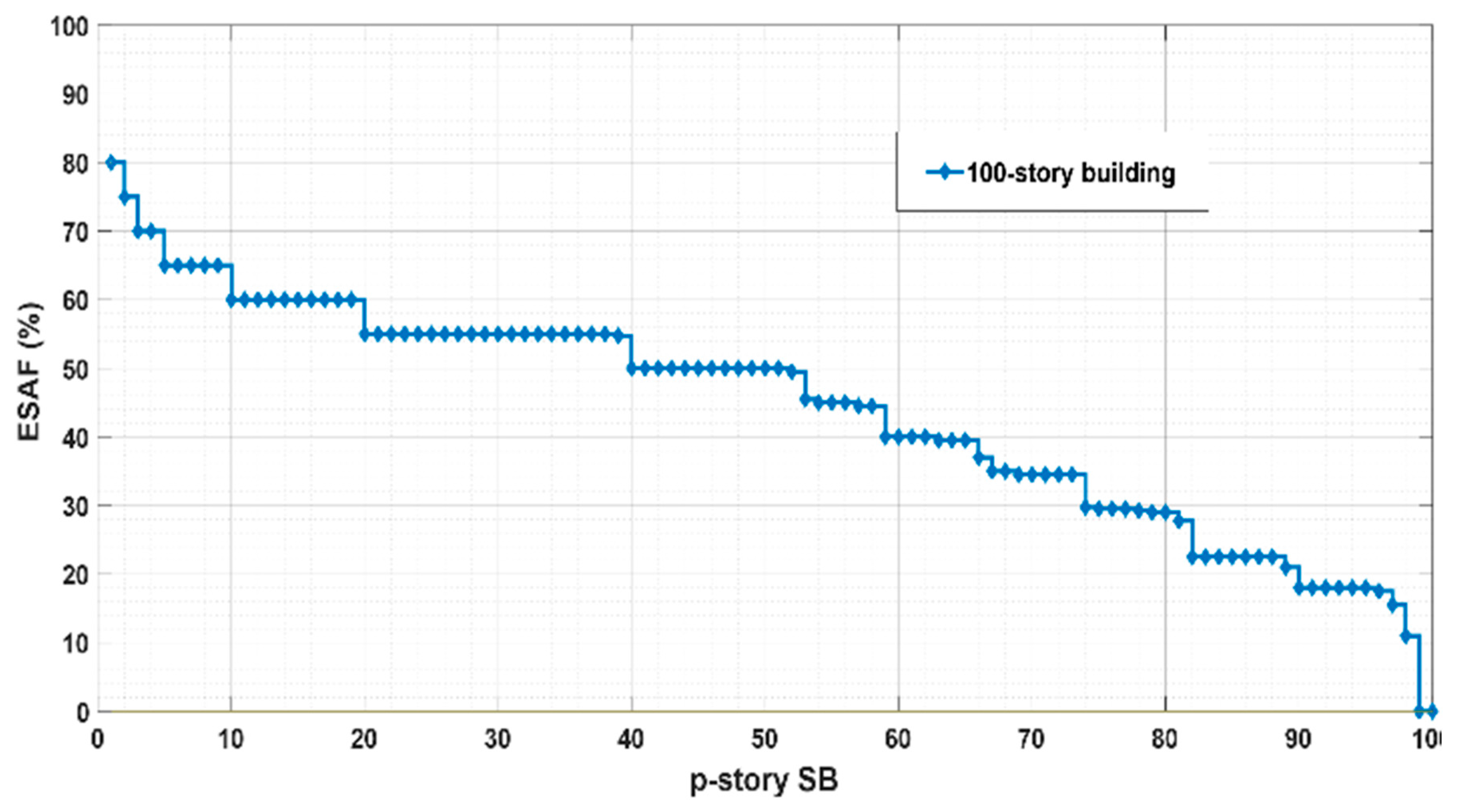
The behavior of the ESAF for a 100-story building is shown in
Figure 12. The effects of the contribution of the reflected rays in the five-ray model can be appreciated when simulating an SB that has more than 50 floors. As expected, the ESAF was high on the lower floors and began to decrease slowly in the upper floors, but after the 50th floor, the ESAF decreased rapidly until reaching zero on the 99th floor.
The rapid decrease in the ESAF occurred because the contribution of the reflected ray began to become significant, and this was because the highest floors of all the SBs were closer to the BS of the primary system. In other words, the power contribution of the rays reflected in the neighboring buildings was high enough to reduce the ESAF. The analysis below focuses on the ESA results for various SBs, whose behavior was related to the SB height and distance to BS.
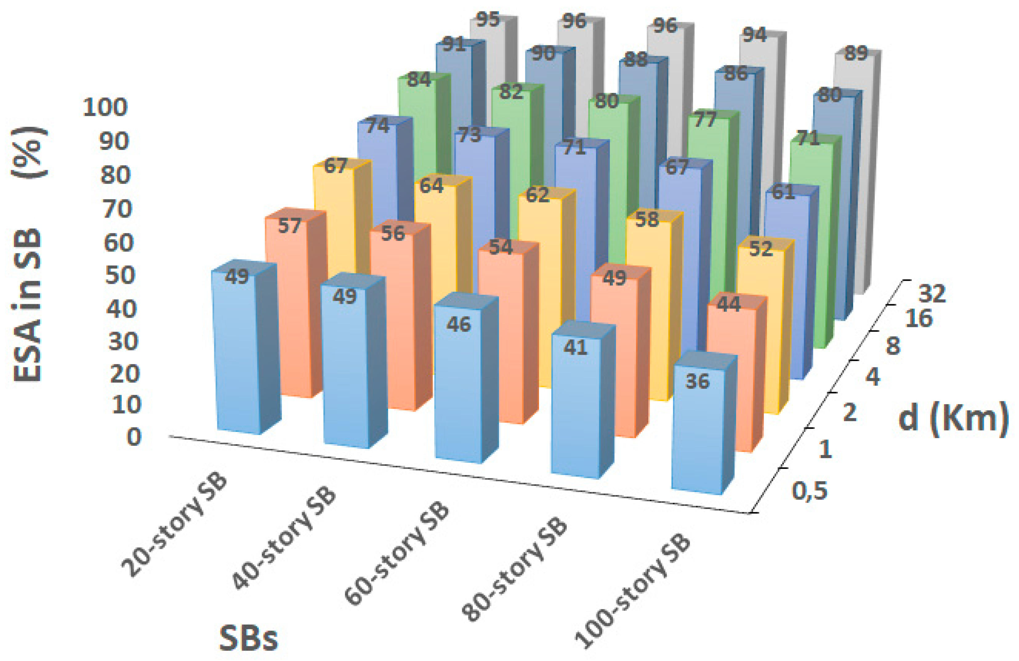
The ESA from a 20-story SB to a 100-story SB when
varied from 0.5 km to 32 km can be seen in
Figure 13.
Figure 13 shows that the ESA for a 40-story SB was distributed through 67% of the total area of the building, while for an 80-story SB, the ESA corresponded to 58% of the total area, and for a 100-story SB, the ESA occupied 52% of the total area of the building when the SB was located 2 km from the BS. Meanwhile, at small
values, a low ESA was obtained, and the ESA grew as
grew.
The same figure shows that the taller buildings had lower ESA values than the smaller buildings for the same distance . This implies that the smaller buildings are more efficient at containing ESA, because as the SB grew, the ESAF decreased. This behavior was maintained regardless of until 16 km, so it can be said that an SB improves its efficiency by between 7% and 9% each time is doubled.
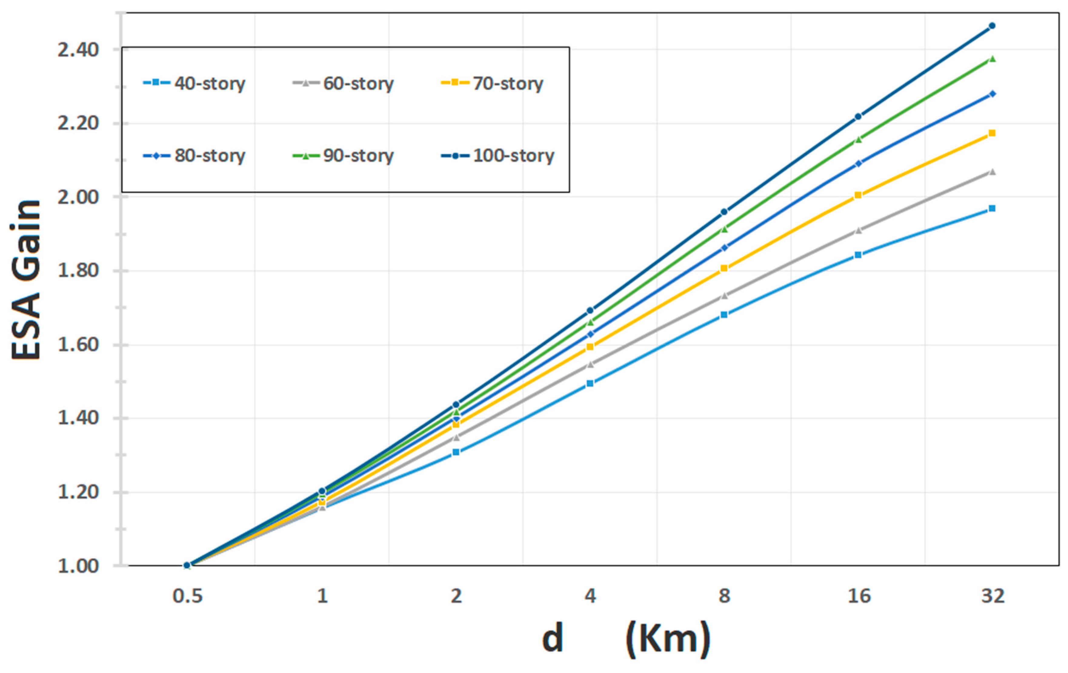
A new SB could be built by considering its inner ESA, as the ESA target of an SB can be achieved by either varying the height of the building or moving it away from a reference point.
Figure 14 shows that the ESA gain when
= 0.5 km can be considered as an ESA reference. This figure shows that a 60-story SB has an ESA gain of 1.16 if the building is moved 0.5 km from the reference point, but the gain will be 2.07 if
is 32 km. However, a 100-story SB will gain 1.20 in the first case and 2.46 in the second case.
In addition to this, the results allow an analysis of the ESA’s gain if a specific building is established as a reference at a specific distance.
Table 3 shows a mapping of the ESA gain that would be obtained according to the locations and heights of buildings, taking a 40-story SB located 0.5 km from the BS as a reference.
To determine the size and location of an SB that has a gain of two times the ESA of the reference, there are several options: locating a 40-story SB 32 km from the primary BS, locating a 50-story SB at d = 8 km, or using another 80 floors located 1 km from the BS.
6. Conclusions
In this paper, the use of a mechanism to determine the ESA inside an SB was shown. This ESA mechanism allows the feasibility of providing proprietary or public services using SR-CRWS inside an SB to be determined in a fast and accurate way, considering that the results were estimated within a CI with a probability of 0.95.
The results obtained indicate that, due to the configuration of the deployment of the PU, no SB reaches 100% ESA efficiency and that the last two floors of the buildings cannot be used for the operation of an CR-based SS. However, those last two floors could be dedicated to the SB control rooms.
Although the mechanism for obtaining the ESA found results for a specific TV channel, it can be said that the spatial availability would be approximately the same for all TV channels if the transmission was made from a single tower, as is the case in several large cities. If not, the results will vary depending on the locations of the BSs.
Within the ESA zone, two or more SR-CRWS could use the same spectrum availability because the SSs support interference up to a given SNR, that is, they self-regulate the use of spectrum availability. However, to differentiate their transmission from the BS transmission, they must use a differentiating element, such as a beacon that identifies all SSs.
As time passes, the spectrum shortage would also threaten the current spectrum bands authorized for the new systems. For this reason, encouragement of the spatial availability of the spectrum is needed if the operation conditions are met. Building interiors are suitable places for reusing unused frequencies, both spatially and temporally. For this reason, SBs could be designed to obtain the desired ESA, which can be achieved by varying the heights and distances from the BS.
This proposed mechanism specifically determines the spectrum spatial availability, so future work in this area should aim to predict the temporary availability of the spectrum inside buildings based on the measurement campaigns and the use of Deep Learning models.


