A Dynamic Path Planning Method for Social Robots in the Home Environment

Abstract

The home environment is a typical dynamic environment with moveable obstacles. The social robots working in home need to search for feasible paths in this complex dynamic environment. In this work, we propose an improved RRT algorithm to plan feasible path in home environment. The algorithm pre-builds a tree that covers the whole map and maintains the effectiveness of all nodes with branch pruning, reconnection, and regrowth process. The method forms a path by searching the nearest node in the tree and then quickly accessing the nodes near the destination. Due to the effectiveness-maintaining process, the proposed method can effectively deal with the complex dynamic environment where the destination and multiple moving obstacles change simultaneously. In addition, our method can be extended to the path-planning problem in 3D space. The simulation experiments verify the effectiveness of the algorithm.

1. Introduction

The co-existence of human and robot will become the main pattern of home environment in the future [1]. Running in the same space with human, the robots are not allowed to collide with human and not expected to interfere with human movement [2]. Therefore, the capacity of motion path planning is pivotal for a robot to run in the home environment.

The purpose of the motion path planning is to find a feasible path from the robot’s current position to the target position without collision with obstacles. The process of planning may realize a series of optimized results e.g., the shortest path length, the lowest energy consumption, or the fastest planning process.

As the home environment is variable, the robot needs a comprehensive perception of the home environment. For example, the robot will build a complete map through SLAM [3,4], including the shape of the room, the position of the furniture, and the walkable area, which are relatively fixed. The robot can plan its path based on the map. However, in the home environment, there are moving obstacles including both small pieces of furniture and moving people. These changing factors will affect the robot’s pre-planned path, making it no longer feasible.

In this work, we mainly consider the path planning of the robot running in the home environment, and propose a dynamic path planning algorithm, so that the robot can, in real-time, adjust the path in variable environments with moving obstacles and changeable destination.

2. Related Works

It is desired that social robots have the ability to move around in the house. The navigation in home environment is a challenge for social robots. A novel algorithm [5] based on the convolutional neural network uses a monocular camera to obtain the location and direction of the door. This method allows the social robots to move among rooms. A novel navigation algorithm for social robots that is acceptable to people is proposed in [6]. By detecting the attitudes of people towards robots, the method establishes the range of influence to generate robot paths that have less impact on human activities.

As the pivotal foundation in social robot navigation, a wide variety of path planning methods have been proposed for robots navigating in different environments [7,8,9,10]. In general, these methods can be divided into global and local methods according to the completeness of map information known before path planning progress. In addition, these methods can also be divided into dynamic and static methods according to the existence of mobile obstacles or not.

The rapidly-exploring random tree (RRT) algorithm extends the tree through collision detection with the obstacles, without modeling the environment [11,12]. Therefore, the RRT method can find feasible paths quickly and effectively for spaces with complex obstacles and high-dimensional spaces which is hard to model. It has been proven that if the path exists, it can definitely be found by the RRT algorithm. However, due to its randomness in the sampling process, the results of the RRT are not the optimal path and vary over time.

In recent years, some improved methods of RRT have been purposed to find feasible paths in changeable environments. The execution extended RRT (ERRT) method proposed in [13] is a real-time planning method, which establishes the waypoint cache to store the feasible path planned in the last time. In the next search, the sampling point will be selected from the target point, random points, or cache points according to the probability. At the same time, the adaptive cost penalty search is proposed to search for the approximately optimized path.

The method proposed in [14] stores the results of the previous planning to have an impact on the next planning. Different from ERRT, this method uses a data structure called the Reconfigurable Random Forest (RRF) to store the tree rather than some waypoints. In the next planning, when the random tree extended near one previous tree stored in the RRF, the two connect into one tree, which will speed up the pathfinding search.

DRRT [15,16] is another real-time pathfinding method applying to the environment with movable obstacles. When the obstacle interrupts the feasible path, the Dynamic Rapidly-exploring Random Trees (DRRTs) will trim the broken branch and re-grow toward the target point, which will generate a new tree. In this method, the invalid branch will be totally abandoned and will not be reused in the next planning process.

To combine the DRRT and the ERRT, the Multipartite RRT(MP-RRT) method was proposed [17]. Similar to the DRRT, when the movable obstacle interrupts the previous path, the MP-RRT trims and cuts down the invalid branch. However, similar to the ERRT, the MP-RRT will not abandon the invalid branch. Therefore, in the next step, the broken part of the tree will re-grow through selecting the sample points from the target, the random points, or the broken branch stored.

Some other local re-planning RRT method can also handle the movable obstacles. Some improved methods [18,19,20] consider the relative motion of robots and obstacles. When the robot finds out that it will collide with an obstacle, the algorithm will set the robot’s current position as the starting point, while the node on the original path which bypasses the obstacle as the target point. It then generates a new random tree to connect the two points and bypasses the obstacle.

Besides the RRT based algorithm, the PRM method is similarly the probabilistic method using the sampling points to search feasible paths. Through random sampling in the workspace and establishing a pairwise connection between all sampling points, a roadmap consists of sampling points and edges is established. The A* or RRT can be used to search in the roadmap to find a feasible path [21]. This method is fast, but need large storage space.

In this work, we propose an improved RRT algorithm to plan a feasible path in home environment. The proposed method greatly increases the pathfinding speed in complex dynamic environments with concave polygon traps, movable obstacles, and changeable destination. Unlike the regrowth algorithms DRRT, ERRT, and MP-RRT, our method does not need to regenerate a new tree on a large scale. In our method, the roadmap is pre-built and only a small scale of new nodes are created to connect broken branches, which speeds up the path searching process. The RRF method uses the tree stored from the previous planning to speed up the tree regeneration speed. However, with the continuous running of the algorithm, the required storage space increases continuously. The algorithm has to sparse the forest by pruning. In the proposed method, the size of the roadmap is limited in a certain map and does not increase as the algorithm runs, which makes the algorithm much cleaner. Different from the roadmap built with PRM, the roadmap in our method is generated by growing a guided tree, which greatly reduces the numbers of edges. The proposed method is suitable for the navigation of wheeled robots and legged robots [22,23,24].

3. Improved Dynamic RRT Algorithm

Aiming at the home environment with movable obstacles, a fast path planning method based on Rapidly-exploring Random Tree is proposed. Inspired by the roadmap method, we maintain a roadmap throughout the whole search space. Just like the highways all over the city, the robot can go anywhere in the space starting from the nearest node in the map. Before the first path planning process, the roadmap has been pre-generated. The only work in real-time planning calculation is maintaining the effectiveness of the roadmap under multiple moving obstacles and selecting a feasible path in the roadmap, which can speed up the path generation process. Besides, since the tree expands to every corner of the map, our method can also cope with the process of the destination changing in real-time.

The key steps of our method include roadmap generation, branch pruning, reconnection, and regrowth. The general process of the method is shown in Figure 1.

In the traditional RRT algorithm, the data structure used to describe the random tree only records the parent node id to reverse trace the source, so as to realize the path generation. We use this idea to generate a feasible path, and expand the data structure to describe the random tree. We introduce the linked list to describe the relationship between nodes, with which we can perform fast forward and backward search as well as root node transformation on the random tree.

The tree in our method is a multi-forked tree with unknown numbers of leaf nodes due to the randomness of the growth process. Each node in the tree has three types of key neighbor nodes, namely its parent node, child nodes, previous node, and the next node at the same level. The linked list with four values, the previous index, the first index at the next level, the previous and the next index at the same level, matches well the characteristics of the multi-forked tree. To create a record for each node, the format is as follows.

$$[parentfirst\_childpreviousnext]$$

(1)

In the record, parent is the node ID of its parent node, first_child is the first node ID at its next level, previous and next are the previous and next node ID at its same level. If a neighbor node does not exist, the corresponding ID will be set to −1. Figure 2a shows the typical form of a random tree. The list in Figure 2b is the linked list of the tree in Figure 2a.

3.1. Roadmap Generation

We use the RRT method to generate a large tree in the search space before the first path search process. First, we select a root node in the feasible area of the map, which does not conflict with the obstacles. The position of the root node does not need special consideration, because the position of the root node will change at any time according to the motion of obstacles.

After selecting the root node, we use the classical RRT method to generate a tree throughout the whole map. To increase the divergence of the tree, the sample points are selected randomly to guide the branches into every corner of the map. The key problem is how to determine that the tree has grown sufficiently and when to stop the growth process.

Inspired by the growth process of plant roots, we propose the Nutrient Indicators to measure the growth of trees. In nature, the roots of plants can bypass stones during stretching into the soil, and can absorb nutrients in the soil within a certain range. When the nutrients in the soil are almost completely absorbed, it indicates that the plant root system has expanded into the entire soil. We simulated this process and the main idea of the Nutrient Indicators is shown in Figure 3.

First, a nutrients matrix is set up according to the map size, and each point in the map corresponds to an element of the nutrients matrix. If a point is in a non-obstacle area of the map, the nutrient of the point is 1; if a point is in the obstacle area in the map, the nutrient of the point is 0. The sum of all elements in the matrix is calculated as the total amount of nutrients of the entire space. During the growth of the random expansion tree, when a new node is generated, the weights of all points in the square neighborhood of the node are set to 0. It means that the newly growing node absorbs nutrition in the surrounding neighborhood. The total amount of nutrients in the space has also decreased accordingly. When the ratio of the current total amount of nutrients to the initial total amount of nutrients is less than the threshold, it is determined that the tree has fully grown and the growth process is stopped.

Besides, when an obstacle in the map suddenly disappears and leave a new free area, the increasing amount of nutrient will restart the tree growth to fill the new free area, which will be introduced in detail in subsequent sections.

3.2. Branch Pruning

When the obstacle moves, some branches will conflict with the obstacle and are no longer feasible. In the step before every new path search process, we must ensure that every branch in the road map is valid. It means the robot can safely reach every corner of the map through the branch. In other words, the reachability of all nodes needs to be maintained. Therefore, we build the Branch Pruning mechanism to cut off the nodes that are no longer valid.

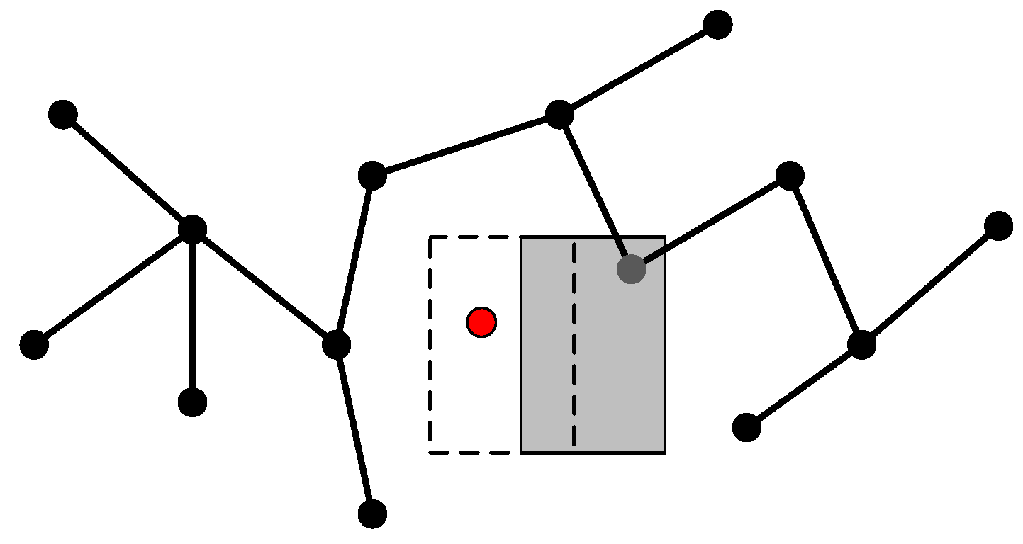
The main idea of the pruning algorithm is shown in Figure 4.

We establish the detection neighborhoods around obstacles and check for leaf nodes that fall inside the area (Algorithm 1 line 1). As shown in Figure 4, two kinds of nodes need to be check, typically node 4 and node 3. Node 4 is just inside the obstacle area, which means it is conflicted with the obstacle and will be set to infeasible directly (Algorithm 1 lines 2 and 7). While node 3 falls inside the check area but outside the obstacle area, so we need to confirm that the connection line between node 3 and its parent node does not pass through the obstacle area (Algorithm 1 lines 4–6). Obviously from Figure 4, the line between the two nodes passes through the obstacle, so the connection between the two nodes will be cut off (Algorithm 1 line 9), node 3 will be separated from the tree as an isolated point. All feasible child nodes of the infeasible node are set as the new root node (Algorithm 1 line 8), as well as the nodes that are broken from their parent nodes (Algorithm 1 line 10).

Algorithm 1 Branch Pruning

Input:$tree$: the list of node coordinates, $treelist$: the linked list Output:$newroots$: the list of new roots that is cut off, $totalNutrient$: the total nutrient in the map 1: $clist\leftarrow$inCheckArea ($tree$) 2: $innode\leftarrow$inObstacle ($clist$) 3: $totalNutrient\leftarrow$IncreaseNutrient ($innode$) 4: if Conflict (($clist-innode$) to ($clist-innode$).$parent$) == true then 5:     $bnode$.add ($clist-innode$) 6: end if 7: BreakLinkedList ($treelist\left(innode\right)$) 8: $newroots$.add (AllChild ($innode$)) 9: BreakLinkedList ($treelist\left(bnode\right)$) 10: $newroots$.add ($bnode$) 11: return newroots, totalNutrient

After the branch pruning process, the whole tree will be cut into several separated parts. Each part becomes an independent tree on the map. At this time, any two trees cannot be connected to each other. Therefore, we propose the reconnection method to connect scattered trees into a complete tree.

3.3. Reconnection

Before path searching, we must ensure that every branch in the map is feasible and reachable. However, due to the moving obstacle, the whole tree is cut off into several separated parts. It will fail when the robot starts searching from one tree while the destination is located in the other tree. Therefore, the separated parts need to be connected.

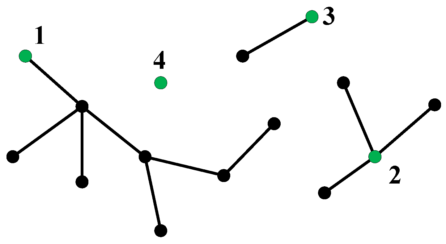
We still use the RRT growth frame to generate a new branch from one tree to another. The connecting process is shown in Figure 5. Tree 1 and Tree 2 are separated trees, and their root nodes are marked as id 1 and id 7. We first generate a random sampling point, shown as the red point in Figure 5, and calculate the distance between nodes in tree 2 and the sampling point to find the nearest node. We get node 9 and grow a step distance towards the sampling point, creating a new node. In the next step, the distances between nodes in tree 1 and the new node are calculated to find the nearest node in the tree 2. In Figure 5, the nearest node is node 5, and if the distance between node 5 and the new node is less than the connective threshold, the two nodes will be connected.

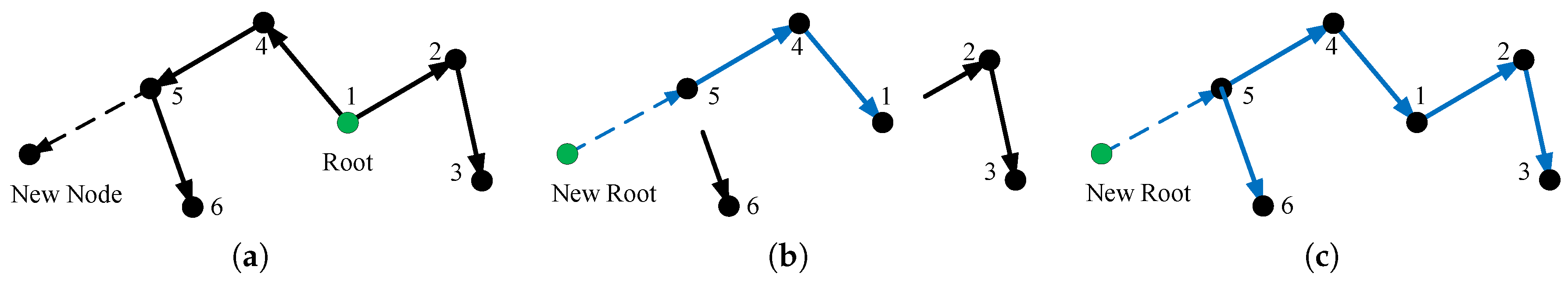
Before connection, the most important thing is to modify the linked list of the merged tree, in order to assimilate into another tree. We propose a method including $traceback$ and $re$-$attach$ steps to merge the two linked lists, which is shown in Figure 6.

• Step 1: $traceback$. We have obtained the new node and iteratively traced back to the parent node through the index, until arriving at the root node and forming the main branch (Algorithm 2 line 1). All child nodes of the main branch, except the child nodes that are already in the main branch, are the sub-branches waiting to be remounted on the main branch (Algorithm 2 line 2). At the same time, modify the parent and child indexes in the linked list of all nodes on this route, while the previous and next indexes are set to −1 (Algorithm 2 line 3).
• Step 2: $re$-$attach$. After the previous step, since the sibling node index of the node is set to −1, only the index of the main branch is recorded on this route. Other branches need to be remounted to the corresponding parent node. During the remount process, the branch firstly checks whether the parent node already has child nodes (Algorithm 2 line 5). If not, we modify the linked list of the parent node (Algorithm 2 line 6), otherwise, we modify the linked list of the last previous node (Algorithm 2 line 8–9).

Algorithm 2 ChangeRoot

Input:$tree$: the list of node coordinates, $newrootId$: the index of new root node, $originalrootId$: the original root node of the tree, $treelist$: the linked list Output:$tree$: the tree after changing, $treelist$: the linked list after changing 1: $Mb\leftarrow newrootId$ to $originalrootId$ 2: $Sb\leftarrow$ AllChildId ($Mb$)-$Mb$ 3: countercurrent ($Mb$) 4: for$i=1$; i < Size ($Sb$); $i++$ do 5:     if $Sb\left(i\right).parent.first\_child==-1$ then 6:         ModifyLinkedList ($treelist$ ($Sb\left(i\right)$.parent)) 7:     else 8:         $lastprevious\leftarrow$SearchLastPrevious ($Sb\left(i\right).parent.first\_child$) 9:         ModifyLinkedList ($treelist$ ($lastprevious$)) 10:     end if 11:     ModifyLinkedList ($treelist$ ($Sb\left(i\right)$)) 12: end for 13: return$tree,treelist$

After the above steps, the tree is attached to another tree and the merger is finished. Usually, obstacles will cut out multiple sub-trees, and the merging order has an important impact on the time consumption of the merging algorithm. As shown in Figure 7, the obstacle cuts out four trees in the map. If we first grow tree 1 to tree 4, due to the small size of tree 4, it may need to sample many times to generate the branch right near the tree 4. However, if we first grow tree 4 to tree 1, the new branch is more likely to be captured by tree 1, because tree 1 takes up more space. Therefore, before merging trees, we always choose the tree with the fewest nodes to start growing (Algorithm 3 line 1). After growing a new node of tree 4, we calculate the nearest node on the other trees, and if the distance is less than the connective threshold, then the connection occurs (Algorithm 3 lines 2–15).

The detailed process of the Reconnection method is shown in pseudo-code.

Algorithm 3 Reconnection

Input:$trees$: the node list of all trees, $map$: the map, $treelist$: the linked list Output:$tree$: the tree after changing, $treelist$: the linked list after changing 1: $tree1\leftarrow$FindShortest ($trees$) 2: $samplepoint\leftarrow$Random ($map$) 3: $nearest1\leftarrow$FindNearestNode ($tree1,samplepoint$) 4: $newnode\leftarrow$Extend ($nearest1,stepsize,samplepoint$) 5: for$i=1$; $i<Size(trees-tree1)$; $i++$do 6:     $ndis\leftarrow$FindShotestDis ($trees\left(i\right)$, $newnode$) 7:     $nNode\leftarrow$FindNearestNode ($trees\left(i\right)$, $newnode$) 8:     if $ndis<ConnectDis$then 9:         ChangeRoot ($tree1$) 10:         ModifyLinkedList ($treelist$ ($nNode$)) 11:         ModifyLinkedList ($treelist$ ($newnode$)) 12:         $trees\leftarrow$ Remove ($tree1$) 13:         break 14:     end if 15: end for 16: return$tree,treelist$

3.4. Pervasive Maintenance

When an obstacle moves through the map, it continuously cuts branches and eliminates invalid nodes. It decreases the number of effective nodes in the map, especially the empty area behind the moving obstacles.

The Nutrient Indicators will perceive this change. When the valid node decreases, the total nutrient of the map increases. If the total nutrient is larger than the threshold, the process of tree growth will start again and creates new branches to fill the empty area(cf. Figure 8).

However, during this growth process, the position of the empty area is accurately known. The random sampling method is not efficient now to fill the empty area quickly. Therefore, our method tends to randomly sample in the empty area. Meanwhile, the growth process needs to maintain divergence, so we set a probability threshold. When the random value between 0 and 1 is higher than the probability threshold, the method randomly samples from the blank area; when it is lower, the method randomly samples from the entire map. The grown method is still based on the RRT frame.

3.5. Path Search and Optimization Processing

All the above methods are run to maintain an effective roadmap spread throughout the map. Through the roadmap, a robot selects the nearest node on the tree and reaches any location on the map. Because the maintenance method can ensure the effectiveness of the roadmap at any time, and the pervasiveness ensures that there can be a branch near the moving target points, it can quickly search for a feasible path in the dynamic environment with a changeable target and multiple moving obstacles.

The path search method is based on the classical RRT algorithm, as shown in Figure 9. The orange point is the location of robot, while the blue point is the destination point. The robot finds the nearest node of the tree as the entrance of the roadmap, then iteratively searches until arriving at the root node(shown as the orange arrow). The process is repeated for the destination (shown as the blue arrow), and the two paths will meet at the root node. As shown in Figure 9, the path from point C to the root repeats in both traceback paths. Our method checks and deletes this duplication.

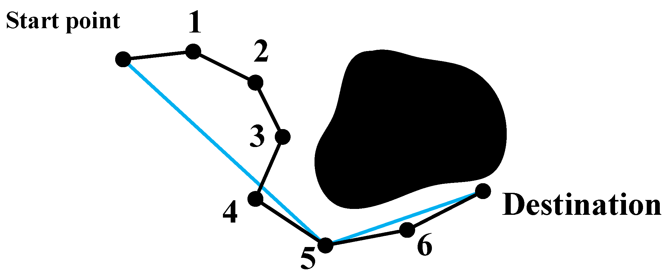
The path calculated by our algorithm is a polyline connected by multiple nodes in which there are a lot of redundant points (as the black line in Figure 10), which is not smooth for a robot to follow directly.

The path starts from the starting point and passes through nodes 1–3 in the process of reaching node 4. However, the straight line between the starting point and node 4 does not pass through the obstacle area, i.e., the robot can travel straight directly to node 4 without collision with the obstacle. The length of the journey direct from the starting point to node 4 is less than the length passing through nodes 1, 2, and 3. Similarly, the path from node 5, passing node 6, to the target node can also be contracted to the straight-line path directly from node 5 to the target point. Therefore, the path result after the contraction calculation is shown as the blue line in Figure 10.

The path contraction algorithm traverses backwards from the starting point to the target point, calculating whether the straight-line path between every point and the starting point collides with the obstacle (Algorithm 4 line 4). We save the last node ID in this search loop without collision and use this node as the starting point of the next search (Algorithm 4 lines 5–6). The search continues backwards to the target point in turn, until the target point becomes the last node without collision in a loop (Algorithm 4 lines 8–10), then the contraction ends.

Algorithm 4 Smooth

Input:$path$: the path searched from the tree, $map$: the map Output:$smoothpath$: the result path after Smooth 1: $currentnodeid\leftarrow$1 2: $smoothpath$. AddNode ($path\left(currentnodeid\right)$) 3: while$currentnodeid\ne$ Size ($path$) do 4:     for $i=currentnodeid$; $i<Size\left(path\right)$; $i++$ do 5:       if CheckConflict ($path\left(currentnodeid\right)$ to $path\left(i\right)$) == false then 6:         $currentnodeid\leftarrow$i 7:       end if 8:       if i == Size ($path$) then 9:         $smoothpath$. AddNode ($path\left(currentnodeid\right)$) 10:       end if 11:     end for 12: end while 13: return$smoothpath$

4. Simulation and Results

This section shows the experimental result and discusses the character of our method. In these experiments, some general settings are established. The program runs in MATLAB R2017b on Dell Inspiron 7590 with Intel i7 CPU at 2.60 GHz. The size of the map is 640 × 480. In the map, the value of the points in the obstacle area is set to 0, while the value in the free space is 1.

4.1. Roadmap Generation Experiment

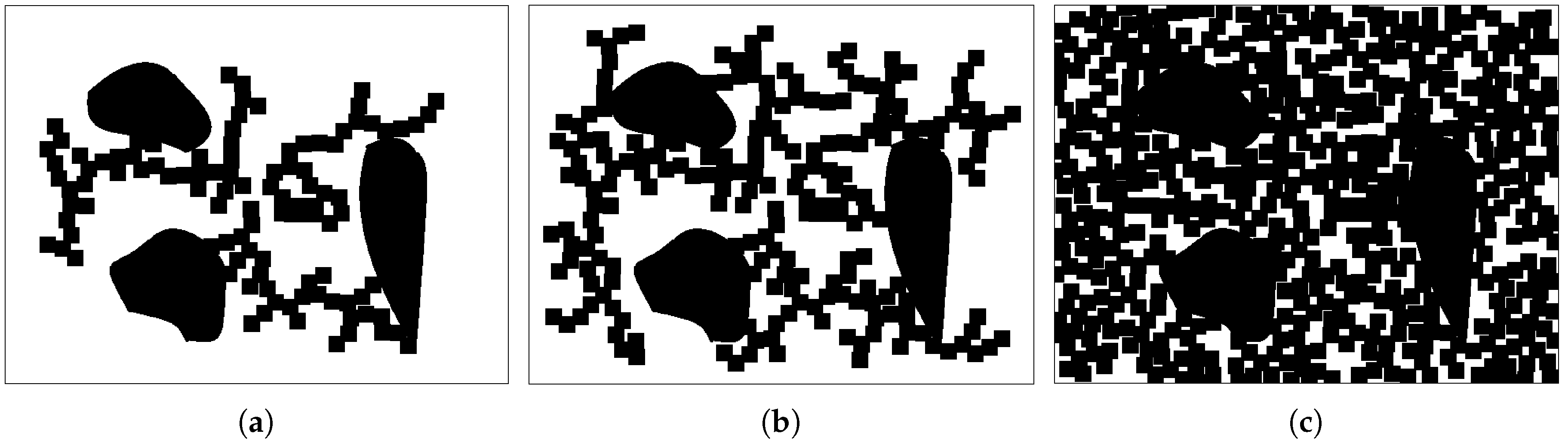
We start growing the tree from point (320, 240), the center of the map. After successfully growing a node as a step, Figure 11 demonstrates the growth process of the tree at the 100th step, the 200th step, and the final step. In the map, the black areas are obstacles, and the rectangle black area is the moving obstacle.

Corresponding to the growth process of the branches, the total nutrient has also changed. As shown in Figure 12, the nutrient distribution changes at the 100th step, the 200th step, and the final step.

With the increase of the nodes, the growth efficiency gradually decreases. Especially in the later process of growth, it may take more sampling times to generate one qualified node. No matter how much time is spent, the algorithm will not cause the tree to grow significantly. The amount of nutrient can reflect this trend. Figure 13 shows the decrease of the total nutrient.

It can be seen from Figure 13 that the inflection point of the descent speed appears around 0.2. When the nutrient decreases below 0.2, the reduced speed slows down, which means the growth process becomes inefficient. The growth process is stopped when the nutrient decreases near 0.2. In our experiment, we select 0.25 as the threshold. The average time for single growth after ten growth experiments is 1.2502 s and the variance is 0.0011.

4.2. Branch Pruning Experiment

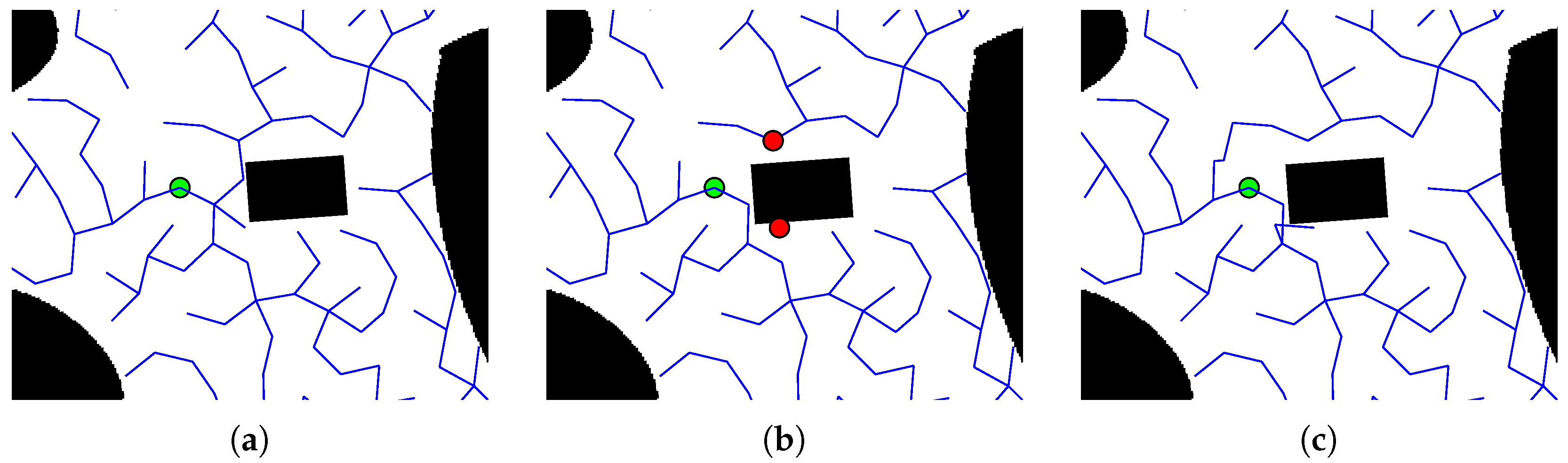
The experiment of the branch pruning process is shown in Figure 14a,b. The green point on the tree is the root node. The red points are the new roots of the subtrees which are created by obstacle cutting.

In this process, the rectangle obstacle moves left and cuts off the branch on the left. This moving obstacle separates the branch in the upper right corner of the map from the main tree and forms a new tree. Meanwhile, a single node under the obstacle is cut off, which becomes a subtree with only one node.

4.3. Reconnection Experiment

After the branch pruning process, the conflict nodes are cut off and several sub-trees are created. Through the reconnection process, the sub-trees are connected into one tree as shown in Figure 14c.

The trees before reconnection are shown in Figure 14b. The sub-tree in the upper right corner is connected to the origin tree through the new node above the green point. Meanwhile, the single point tree is connected through the new node below the green point. Therefore, all of the subtrees are merged and restored into a completed single tree.

During the merging process, the sub-trees are needed to change the root node in order to mount on other trees. The experiment about root change is shown in Figure 15.

4.4. Pervasive Maintenance Experiment

After the obstacle moving, the blank area behind the obstacle is filled by growing a new branch, as the branch shown in Figure 16b under the obstacle. We set the upper nutrient threshold to 0.25, which means if the nutrient increases above 0.25, the regrowing process will start.

4.5. Path Search Experiment

To verify the performance of the proposed algorithm, we develop a complex environment consists of walls, a static rectangular obstacle, a static obstacle with irregular shape, and three movable rectangular obstacles. Besides, the destination of robot changes over time. There are some challenges in this map: the narrow corridor around the static rectangular obstacle, traps of the concave polygons formed by walls, and the moving obstacles. Corresponding to the home environment, the static rectangular obstacle represents a table or a cabinet. The irregular obstacle represents irregularly shaped furniture such as a sofa. The moving obstacles represent humans or pets. The narrow corridor and the trap formed by furniture and walls are common in the home environment.

We test the performance of three dynamic RRT methods in this map: ERRT, the Smoothly RRT (SRRT) proposed in [18], and the proposed method in this work. The map size is 640 × 480. The starting point of the robot is $(10,10)$. The whole process of the robot moving from the initial point to the destination is simulated as one loop. The moving trajectories of obstacles are the same among all loops in three methods. Each loop consists of 30–40 replanning steps and terminates when the distance between robot and destination is within the threshold. In each step, the robot plans a feasible path from the current position to the destination. 10 loops of each method are conducted to test the time consuming of finding a feasible path in one replanning step and the quality of the generated path. 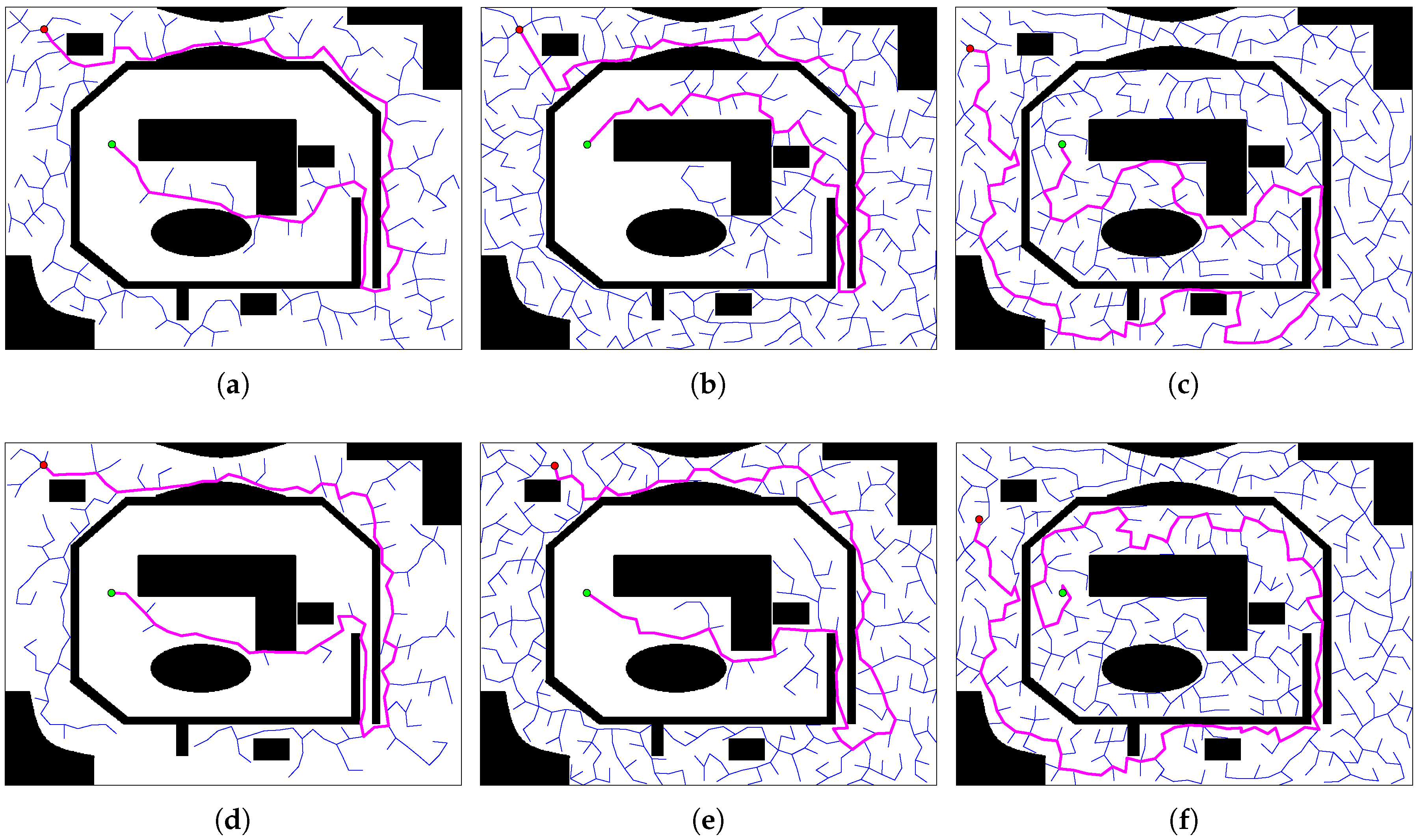Figure 17 shows the paths of two adjacent steps, where the obstacles interrupt the path of the previous step, and the three methods replan the paths in the next step.

The average time of finding a feasible path in a single replanning step, the average and standard deviation of the total number of path nodes in a single loop are listed in

Table 1. Simulation comparison result of three algorithms.

Experiment	Average Time of Finding Path/ms	Average Node Count	Standard Deviation
ERRT	264	2542	89
SRRT	1446	2827	121
Proposed Method	31	3032	235

.

The results of the 9th, 10th, and 15th steps in one experiment of the proposed method are shown in Figure 18. The pink line is the feasible path generated from tree, while the blue line is the path after contraction. The blue line is the path that robots actually perform.

To fully test the performance of algorithms, we design another map to conduct the experiments of three methods. The size of map 2 is 640 × 480. The starting point of the robot is $(10,10)$. The moving trajectories of obstacles and destinations are designed according to the new map. Other settings of the experiment are not changed. Figure 19 shows the paths of the second and third steps in three methods.

The average time of finding a feasible path in single replanning step, the average and standard deviation of the total number of path nodes in a single loop are listed in

Table 2. Simulation comparison result of three algorithms.

Experiment	Average Time of Finding Path/ms	Average Node Count	Standard Deviation
ERRT	439	1292	82
SRRT	2416	1500	217
Proposed Method	45	2830	631

.

5. Discussion

5.1. Analysis and Evaluation

The proposed method is much more efficient than the ERRT and SRRT to generate a feasible path in complex environments. At the beginning of one loop, a large number of nodes are generated by ERRT and SRRT to explore the map. In Figure 17a,b, the trees generated by ERRT and SRRT almost fill the entire map, which are the same size to the tree formed by the proposed method. In Figure 19a,b, the ERRT and SRRT generate a large number of nodes to find the narrow entrance. The results indicate that the ERRT and SRRT spend a lot of time growing nodes to bypass the moving obstacles, moving out of the traps, and getting through the narrow aisles. As the robot gets closer to the destination, the efficiency of ERRT and SRRT gradually increase. The experiments indicate that ERRT and SRRT are more efficient in simple environments.

However, since the tree is pre-built, the proposed low overhead algorithm does not need to grow a new tree on a large scale in the real-time operation process. A few nodes are needed to be extended in the reconnection process to realize tree merging. The linked list mechanism ensures the fast root transformation, subtree reconnection, and path search. Therefore, the proposed method greatly increases the speed of path discovery in complex environments. In the last few steps of one loop, the robot is close to the destination. At this time, the path discovery speeds of ERRT and SRRT are similar to the proposed method. This result indicates that the proposed method has a limited improvement effect on the path discovery speed in simple environments.

The total node count in a loop reflects the path quality. The paths generated by the proposed method are longer than the ERRT and the SRRT. During the movement of the robot and the destination, the proposed method and the SRRT method select the path independently between adjacent time frames, which may cause a significant change of the path between two adjacent replanning processes. Especially in map 2, there are two directions from the robot’s current position to the destination. The proposed method and the SRRT method may switch between two directions sometimes. The ERRT method uses the result of the previous planning process to guide the current planning process, which causes similar paths between two frames.

In general, the proposed method is valuable for the greatly increment about the path discovery speed in complex dynamic environments with moving obstacles and a changing destination. In the home environment, the social robots may build the static map with SLAM and detect the moving obstacles with the sensors onboard. After building the tree, the effectiveness of all the nodes on the tree is maintained through the proposed method. The robot finds the feasible path to the destination efficiently and performs tasks such as operating switch, following kids, checking rooms, and automatic charging.

5.2. Extension

In the experiments, the robot moves on the ground and its position is $(x,y)$. For some scenarios of UAV and manipulator, the path-planning problem needs to be solved in 3D space. The proposed method can be expanded into 3D or higher dimension space. For the robot moving in 3D space with position $(x,y,z)$, the method selects a root node at $(x_0,y_0,z_0)$ and grows new node $(x_n,y_n,z_n)$ under the guidance of sampling point $(x_r,y_r,z_r)$. The new nodes absorb nutrients from the cube neighborhood. As the growing process runs, the tree fills the entire space. When an obstacle moves, the method checks the nodes in its cube neighborhood and prune the branch. The subtrees are reconnected into one tree by the reconnection steps. Through the roadmap in 3D space, the method selects a feasible path between the robot position and the destination.

Due to the ubiquity of the tree, more store spaces are required and the search time also increases accordingly. By adjusting the sparseness of the entire tree, the number of nodes can be reduced to a certain extent while the effect of the algorithm can be guaranteed.

The proposed method can be applied to the multi-robot path planning process. Each robot treats other robots as obstacles and executes an independent planning method. The conflicts among robots can be solved.

6. Conclusions

In this work, we propose an improved low overhead RRT algorithm that can greatly increase the path planning speed for social robots in home environment. The proposed algorithm pre-builds a roadmap with the RRT method and maintains the effectiveness of all nodes with branch pruning, reconnection, and regrowth process. With this roadmap, we can get a feasible path between the robot and the destination quickly. When the obstacles and the destination are changing randomly, our algorithm will search a feasible path from the robot’s current position to the destination in real-time. The simulation experiments verify the effectiveness of the method.

The proposed method still has some limitations. Because of the randomness of the tree growing process, the RRT frame is difficult to find the optimal path. In addition, the paths planned between two adjacent replanning processes may change significantly. In a future step, we will focus on finding the solution as optimal as possible and try to introduce the heuristic search into the proposed framework to reduce the path variation. Besides, we will implement the proposed method on physical social robots in real scenarios such as home environment and hospital environment [25], to evaluate the human–robot interaction metrics including technical system performance, user acceptance, user experience, and impact on the quality of life [26].