Measuring the Impact of Accurate Feature Selection on the Performance of RBM in Comparison to State of the Art Machine Learning Algorithms

Abstract

The amassed growth in the size of data, caused by the advancement of technologies and the use of internet of things to collect and transmit data, resulted in the creation of large volumes of data and an increasing variety of data types that need to be processed at very high speeds so that we can extract meaningful information from these massive volumes of unstructured data. The process of mining this data is very challenging since a lot of the data suffers from the problem of high dimensionality. The quandary of high dimensionality represents a great challenge that can be controlled through the process of feature selection. Feature selection is a complex task with multiple layers of difficulty. To be able to grasp and realize the impediments associated with high dimensional data a more and in-depth understanding of feature selection is required. In this study, we examine the effect of appropriate feature selection during the classification process of anomaly network intrusion detection systems. We test its effect on the performance of Restricted Boltzmann Machines and compare its performance to conventional machine learning algorithms. We establish that when certain features that are representative of the model are to be selected the change in the accuracy was always less than 3% across all algorithms. This verifies that the accurate selection of the important features when building a model can have a significant impact on the accuracy level of the classifiers. We also confirmed in this study that the performance of the Restricted Boltzmann Machines can outperform or at least is comparable to other well-known machine learning algorithms. Extracting those important features can be very useful when trying to build a model with datasets with a lot of features.

1. Introduction

The progress in streaming analytics, internet of things, artificial intelligence, signal processing, cloud and cognitive computing, and other technological fields facilitated our access to large magnitudes of data that were not available in the past. This surge, coupled with the rapid growth in the dimensionality of the data and its volume has created new-found challenges. These large sets of data along with the analysis requirements that transpired with them to uncover hidden patterns and unknown correlations came to be known as “Big Data Analytics”. The benefits gained from the analysis of big data affects nearly every field out there. The approaches and methods used to analyze and deal with big data are different from the rules used to deal with conventional data, so we need new and innovative approaches and algorithms to extract useful and sensitive information.

Some studies addressed the problem of big data from the volume viewpoint only and failed to address the problem of the massive growth in dimensionality. The problem of the rise in high dimensionality can sometimes prove to be more important and challenging than any elevation in the volume of the data. In some cases, the number of features could even exceed a million, a phenomenon known as feature explosion [1]. Different preprocessing approaches were developed to deal with the problem. Many of those approaches involved various methods. One of those most instrumental methods used was feature selection which is considered a vital step during the analysis of the data and when building predictive models while exploring the relations between many of its features.

One of the main objectives when designing an anomaly network intrusion detection system (A-NIDS) is to be able to build a predictive model that can identify attacks through classifying the network traffic into normal or anomalous behavior. This explains why feature selection techniques are a key factor in creating solutions that reduce the complexity of the data without much loss of the essential parts of the information that are integral to achieve the goal of a faster and more accurate anomaly detection system with higher sensitivity and specificity.

2. Previous Work

Alom et al. [2] investigated the capabilities of Deep Belief Networks (DBN) by training a sequence of Restricted Boltzmann Machines (RBMs) and evaluating their performance against a DBN-Support Vector Machine (SVM) utilizing the NSL-KDD (Network Security Laboratory - Knowledge Discovery in Databases) dataset. Salama et al. [3] explored the use of DBN based on RBM for feature dimensionality reduction on the NSL-KDD dataset. Dhanabal, L. [4] explored the relationship between the protocols in the NSL-KDD dataset and the effectiveness of the various classification algorithms in detecting the anomalies in the network traffic patterns. Belavagi [5] studied the effect of building a model using different classification algorithms specifically random forest, Gaussian naive Bayes, Support Vector Machine, and logistic regression on the NSL-KDD data set and found that random forest outperforms other algorithms in identifying network traffic as normal and attack. For more recent work on utilizing the NSL-KDD dataset for building A-NIDS and a comparison of the different techniques used we refer the reader to this survey study [6] and review paper [7].

3. Methods

3.1. Restricted Boltzmann Machine

The Restricted Boltzmann Machine (RBM) has been proposed in the ’80s but was not heavily utilized due to time and computational constraints. With the recent advancement in high-performance computing, many researchers and specialists in the field of machine learning, pattern, sound, and image recognition [8,9,10,11,12,13,14,15], confirmed that an RBM has a very great and powerful capability to learn complex patterns of data with high levels of accuracy even in the presence of high dimensional features of visual and auditory patterns.

An RBM is a stochastic artificial neural network that consists of one layer of visible units that represent the observable data and another layer or layers of hidden units that represent the relationships between those data units. They are connected through edges that have a specific weight associated with it. In the restricted form there are no direct connections between units of the same type [16,17]. An RBM consisting of m visible nodes $\mathit{v}=\left(v_1,v_2, \dots , v_m\right)$, and n hidden nodes $\mathit{h}=\left(h_1,h_2, \dots , h_n\right)$ can be described in terms of the energy function

$$E\left(\mathit{v},\mathit{h}\right)=-{\mathit{h}}^T\mathit{W}\mathit{v}-{\mathit{b}}^T\mathit{v}-{\mathit{c}}^T\mathit{h},$$

(1)

where $\mathit{W}$ represents the weights, $\mathit{b},\mathit{c}$ representing the bias fields acting on the nodes of visible and hidden units, respectively. The stochastic evolution of the model is governed by the joint probability distribution

$$p\left(\mathit{v},\mathit{h}\right)=\frac{1}{Z}{e}^{-E\left(\mathit{v},\mathit{h}\right)},$$

(2)

where $Z={\sum }_{\mathit{v},\mathit{h}}{e}^{-E\left(\mathit{v},\mathit{h}\right)}$ is the partition function.

To capture the essential features that we are interested in, we need to adjust the internal parameters (i.e., weights and biases) to tune the RBM based on samples from a target probability distribution. Once the RBM is trained, it can act as a generative model that facilitates sampling from the target probability distribution. Hidden nodes will be able to capture relations that are not usually modeled via direct pairwise interaction between pairwise interactions.

During training, the weights and biases of the RBM are continuously adjusted such that its marginal probability distribution fits the training data as well as possible. This is usually done through maximizing the likelihood or the probability $ℒ\left(\mathit{\theta }|X\right)$ of the training data set $X$ given the model parameters $\mathit{\theta }=\left\{\mathbf{W},\mathbf{b},\mathbf{c}\right\}$ [8,18,19]. Maximizing the log-likelihood analytically is considered to be a hard problem so it is usually achieved using the gradient descent method on the log-likelihood. The calculation of the derivative of the log-likelihood in each iteration of the algorithm is the most computationally intensive step of the gradient descent method, which, for a single vector $\mathit{v}$, takes the form

$$\begin{array}{ll}\frac{\partial }{\partial \mathit{\theta }}\left(\log ℒ\left(\mathit{\theta }|\mathit{v}\right) \right)& =-{{\displaystyle \sum }}_{\mathit{h}}p\left(\mathit{h}|\mathit{v}\right)\frac{\partial E \left(\mathit{v},\mathit{h}\right)}{\partial \mathit{\theta }}+{{\displaystyle \sum }}_{\mathit{v},\mathit{h}}p\left(\mathit{v},\mathit{h}\right)\frac{\partial E \left(\mathit{v},\mathit{h}\right)}{\partial \mathit{\theta }}\\ & =-{\langle \frac{\partial E \left(\mathit{v},\mathit{h}\right)}{\partial \mathit{\theta }}\rangle }_{\mathrm{data}}+{\langle \frac{\partial E \left(\mathit{v},\mathit{h}\right)}{\partial \mathit{\theta }}\rangle }_{\mathrm{model}}\end{array}$$

(3)

The first term in Equation (3) is usually referred to as the data-dependent expectation and represents the expectation of the derivative of the energy function under the conditional probability distribution of the hidden nodes given the training vector. The second term, known as the model’s expectation, represents the expectation of $\frac{\partial E}{\partial \mathit{\theta }}$ under the model’s probability distribution over all visible and hidden nodes. It takes exponential time to compute the expectations of the visible and the hidden nodes. Therefore, we commonly use Markov chain Monte Carlo methods [15] to estimate these expectations by drawing samples from the corresponding probability distributions.

For an RBM, due to the conditional independence of the units of the same layer, we can simplify the data-dependent and model-dependent expectations using factorization of the conditional probabilities. Thus, the derivative of the log-likelihood in relation to the weights $w_{ij}$ can be reduced to

$$\frac{\partial }{\partial w_{ij}}\log ℒ\left(\mathit{\theta }|\mathit{v}\right)=p(h_i=1|\mathit{v})v_j-{\displaystyle \sum }_{\mathit{v}}p\left(\mathit{v}\right)p(h_i=1|\mathit{v})v_j$$

(4)

Similarly, the log-likelihood derivatives for the bias $b_i$ of the i^th visible node and the bias $c_j$ of the j^th hidden node are, respectively, given by

$$\frac{\partial }{\partial b_i}\log ℒ\left(\mathit{\theta }|\mathit{v}\right)=v_i-{\displaystyle \sum }_{\mathit{v}}p\left(\mathit{v}\right)v_i$$

(5)

and

$$\frac{\partial }{\partial c_j}\log ℒ\left(\mathit{\theta }|\mathit{v}\right)=p(h_j=1|\mathit{v})-{\displaystyle \sum }_{\mathit{v}}p\left(\mathit{v}\right)p\left(h_j=1|\mathit{v}\right)$$

(6)

Granting that the first term in each of the above three equations can be calculated accurately, precise computation of the second term is still difficult and intractable as it requires summing over all possible visible vectors and hence needs to be estimated through Gibbs sampling [10]. The training process of the RBM by iteratively adjusting the model parameters to maximize the log-likelihood can be achieved through contrastive divergence [20] and persistent contrastive divergence [21] algorithms. These algorithms utilize Markov chain Monte Carlo for estimating the aforementioned intractable terms. Contrastive divergence uses Gibbs sampling to estimate log-likelihood derivatives of a RBM. Adjusting the model parameters a few times during RBM training is sufficient to get the Markov chain to converge to the joint probability distribution of the desired system. In Persistent Contrastive Divergence (PCD) the underlying assumption is that for small learning rate there will be only a slight change in the model parameters, which, in contrast to Contrastive Divergence (CD), avoids the need to reinitialize the Markov chains with training vector ${\mathit{v}}^{\left(0\right)}$ after each parameter update. This allows in most cases the Markov chains to approach thermal equilibrium faster.

3.2. The Other Algorithms

Those algorithms are the J48, which is a very widely used machine learning algorithm created through implementing the C4.5 algorithm in the Java language [22,23]. Naive Bayes [24] based on Bayes’ theorem [25,26] and NB tree, which is a hybrid algorithm variation of the naive Bayes that deploys it on the leaf node of the decision tree and is used to weaken the attribute independence assumption of naive Bayes [27]. Random forest constructs several decision trees and outputs the class that is the mode of classes or mean prediction of the individual trees and is considered a very powerful algorithm due to its ability to correct the overfitting problem that is commonly observed when using decision trees [28,29,30]. Random tree works by constructing a tree that considers K randomly chosen attributes at each node. Multi-Layer Perceptron (MLP) consists of input, output, and one or more hidden layers where each node within each layer has a certain weight and is connected to the other nodes in the next layer through a linear or a nonlinear activation function, it is well known for its ability to distinguish data that is not linearly separable [31,32,33]. In Support Vector Machine (SVM) points or input vectors are mapped to a high-dimension feature space in a non-linear fashion and we want to find a linear classifier using a hyperplane that can provide the maximum separation or margin between the points or vectors belonging to each class and the hyperplane [34,35,36].

4. The NSL-KDD Dataset

Finding a dataset that reflects real-world network traffic flow without any sort of alteration or modification is a big challenge that the researchers of the cybersecurity community are continuously faced with during their evaluation of any NIDS. The problem has been discussed in many papers and research venues [37,38,39,40,41,42]. This problem can be traced back to the fact that companies and institutions do not allow recording, monitoring, or sharing of their private data due to laws related to privacy and confidentiality regulations. Even companies that allow their data to be shared will severely alter and anonymize their data before releasing it to the public, causing the data to lose a lot of its essential components that are indispensable for the researcher to be able to draw logical inferences that are of value to his research.

KDDCup99 is a set of simulated network traffic data that contains around 4.9 million records, each record (i.e., vector) contains 41 features [43]. The data set has been used for a long time as a basis for evaluating network intrusion detection systems even thought inherent problems were reported during the early stages of its usage [44]. Nearly a decade later, The NSL-KDD dataset was created by extracting certain fields from the KDD data set as a means to solve some of the problems that were associated with the KDD data set [37]. Other data sets gained popularity around the same time, one known example is the gureKDDcup [45], which is perceived, along with the NSL-KDD, as an improved alternative than the KDD data set. The NSL-KDD does not solve all the issues associated with the KDD data set, but it is considered a great enhancement compared to its predecessor. The advantages of using NSL-KDD over KDD can be summarized in the following points:

• Redundant records were removed from the training set to omit biases of the classifiers towards those records.
• Duplicated records are not included in the test set to remove the biases of the learners caused by methods with higher detection rates on frequent records.
• The number of records in the NSL-KDD is chosen by sampling a higher percentage of records for each group with higher prediction difficulty level—the groups are categorized into different levels based on how hard it is for the learners to correctly predict the correct class (normal/anomaly) the data set falls under—and are a lower percentage of the total records in the original data set. This approach allows more accurate evaluation when applying different learning techniques on the data.
• The number of records is reasonably small compared to the original dataset to enable one to run the experiments on the whole dataset, without the need to select a smaller subset of the dataset.

5. Data Set Preprocessing

Since we plan to train the data sets using either contrastive divergence or persistent contrastive divergence algorithms. We need to convert the network traffic data into its corresponding binary form to train the machine learning algorithms effectively. It is essential to be certain that the size of the resulting vectors for each data set maintains the same order as the original data to maintain effective training of the data. Good preparation of the data will result in the production of valid and reliable models. Preprocessing the data in most cases will require all or some of these steps, data cleaning, integration, transformation, reduction, and discretization. For the NSL-KDD removal of invalid records was performed during the cleaning phase and selection of some records from the original KDD data set that can be representative of the whole data set was performed during the reduction phase. The NSL-KDD set contained 125,973 training data and 22,544 testing data. This left us with one main challenge when processing the data, which is how well we can discretize the data without much loss of the important information that we need?

When discretization is used properly it can speed up and simplify the process of learning [46]. It is important to note here that the usage of discretization is not mandatory at all times and in fact in some cases, it can have major drawbacks if not properly used or if it is used on data were discretization is not needed. The main barrier when utilizing any discretization technique is to determine a cut point that divides a specific range into a set of distinct intervals that are coherent and without losing much information throughout the process [47]. The discretization of continuous data is of fundamental importance to the process of feature selection. Failure to do so will lead to major flaws in the analysis of the data. Classifier algorithms have different sensitivity levels with regards to the extent at which they are affected by discretization. However, the correct usage of discretization is essential to extract meaningful information from the data.

To discretize the data correctly we need to identify the types of data associated with each feature, and which features require discretization and which ones do not. When analyzing the data we found that we have 41 features in total, they are divided into 34 features that consist of real values, 4 features are binary (i.e., 0 or 1) and 3 features are nominal values excluding the last feature (i.e., feature number 42, which is to label the data as either normal or anomalous). Regarding the binary and the nominal features, no discretization of the data is required. Since these data can be mirrored easily to their equivalent binary form there is no need for any additional data preprocessing.

For the nominal data, the conversion can be done on a feature by feature basis through enumerating the number of different instances in each feature and then mapping each unique instance of the data to a different binary value. If we take, for example, the feature called “protocol type”. This feature contains three different instances TCP (Transmission Control Protocol), UDP, (User Datagram Protocol) and ICMP (Internet Control Message Protocol). To convert this feature to its binary equivalent we simply map TCP to 00, UDP to 01, and ICMP to Then we repeat the same process for all the nominal features within this dataset.

Table 1. Nominal features mapping into a binary representation.

Protocol Type	Binary Value	Service	Binary Value	Flag	Binary Value
TCP	0	Aol	0	OTH	0
UDP	1	Auth	1	REJ	1
ICMP	10	Bgp	10	RSTO	10
		Courier	11	RSTOS0	11
		csnet_ns	100	RSTR	100
		Ctf	101	S0	101

illustrates the conversion of the data instances for the three different nominal features of the NSL-KDD.

For real values, conversion to binary can be a more challenging task. The direct conversion of real values to binary is not feasible. The reason for that can be denoted by the fact that decimal point representation requires more storage space (i.e., more bits per each value) than normal integer values. Moreover, the presence of the decimal point makes it more difficult for the algorithm to learn since there are many instances of values associated with each number. This will increase the size of each record and as a consequence will lead to an increase in the computational complexity required by the model to learn each record and will slow the algorithm’s performance.

Discretization of the data by converting the continuous data into a form of distinct data ranges can be done in numerous different manners and using a wide variety of approaches. This makes the discretization process a challenging task that requires a thorough understanding of the dataset characteristics to allow us to choose the most effective discretization approach. Our goal here was to discretize the data with minimal loss of information. For this data, we chose to discretize the real values in a supervised fashion taking into account the normal and anomaly class labels of the data. After discretizing the data, the ranges were converted into an equivalent integer representation and then into binary values.

If we take on those features for example the feature called “count” (this feature represents the number of connections to the same destination host as the current connection in the past two seconds), the feature is the twenty-third of the KDD data set features. The feature numeric values range from 0 to discretizing this feature in a supervised manner for the normal and anomaly classes will result in creating 28 different ranges of the real values, we will refer to those new ranges as bins.

For each one of the bins created we assigned a numeric value usually in a similar order as the original real values of the discretized range. Then we took those numeric values and converted them to their corresponding binary value while maintaining and preserving their original order to allow for a meaningful comparison. An example of such conversion is shown in

Table 2. Bins assigned integer values and then converted into the binary form.

Feature Name (Count)	Integer Value	Binary Value
(-inf–1.5]	0	00000000
(1.5–2.5]	1	00000001
(2.5–5.5]	2	00000010
(5.5–10.5]	3	00000011
(10.5–13.5]	4	00000100
⋮	⋮	⋮
⋮	⋮	⋮
(502.5–inf)	27	00011011

.

6. Feature Selection

Using all the features in a dataset to train an algorithm for learning and classifying patterns and tasks do not always lead to the most optimal results. This can be simply attributed to the fact that not all the features within a dataset play an active role in the classification task. Knowing which features are important can lower the complexity of the problem, and as a result, increase the performance of many machine learning algorithms. Feature selection can be a very challenging and complex approach. That is why careful selection of certain features over other ones is instrumental to the process of building an accurate predictive model. The difference between determining the importance of each feature can be mainly attributed to the way each algorithm determines or ranks which features are essential and helpful to the model.

For the features selection step to be very effective, we have to consider how each feature functions individually and how it operates when placed as part of a group of features. For example, some features might perform poorly when chosen individually but they might behave in a completely different manner when combined with other features as part of a group. Those characteristics of each feature cannot be identified without such an interaction. That is why appropriate feature selection is considered one of the most essential steps in data preprocessing. To be able to perform such a task correctly we are not only concerned with finding the important features but in many cases finding features that might work better when grouped with other features. For such reason, appropriate feature selection is considered one of the most essential steps in data preprocessing.

Different studies on the KDDCup99 and NSL-KDD data sets have specified different features as important, but most of those studies agree on some features as having more significance as well as having more impact on the classification process, especially when determining which network traffic records incorporate normal behavior and which ones incorporate anomalous behavior.

For the NSL-KDD dataset, the impact of the 41 features on the classification task varies, some features play a significant role in the process, like the type of service (i.e., feature number 3), while others have no real impact and have no significant role like the number of outbound commands (i.e., feature number 20). This does not imply that outbound commands are not an important feature in the classification of network traffic data. It just means that for this specific data set this feature does not play a major role in the classification process.

We chose to use the infoGain [48] algorithm, which is of the filter type feature selection algorithms. Features are ranked in descending order with the most important feature getting the highest score based on the algorithms scoring system. Using the infoGain algorithm we created two new supplementary datasets in addition to the original dataset. The original dataset includes all the features of the NSL-KDD data set. The second data set contains features with the top 22 scores, and the third set contains features with the top 12 scores.

7. Parallelization Strategy

The most computationally intensive step of the gradient descent algorithm for training RBMs is the calculation of the log-likelihood derivatives during each iteration of the algorithm. This can be seen in particular when the size of the RBM is large (i.e., there is a large number of visible and hidden nodes in each layer). The speed at which this task can be performed is a crucial factor that determines the effectiveness of a real-time anomaly detection system.

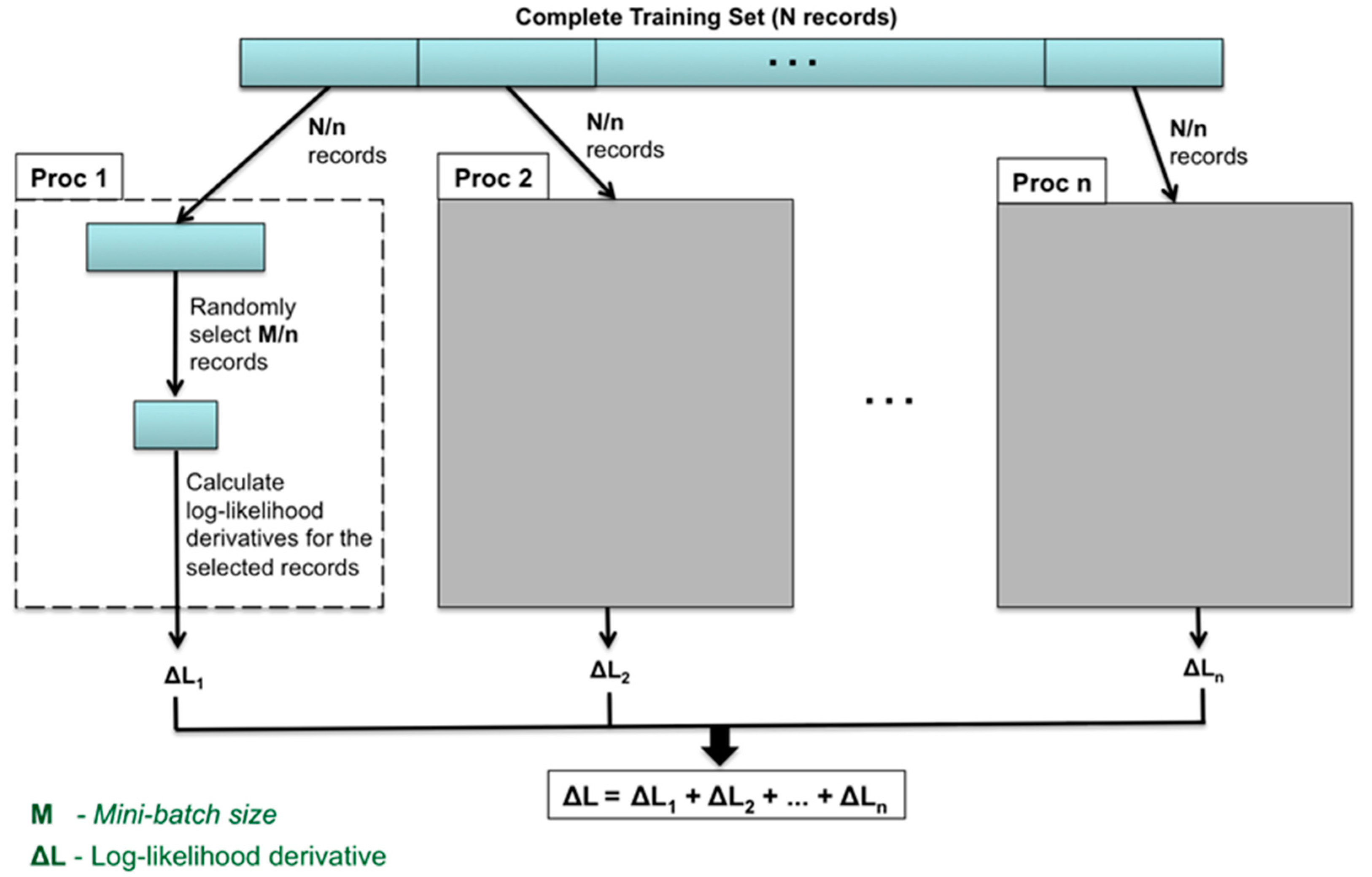
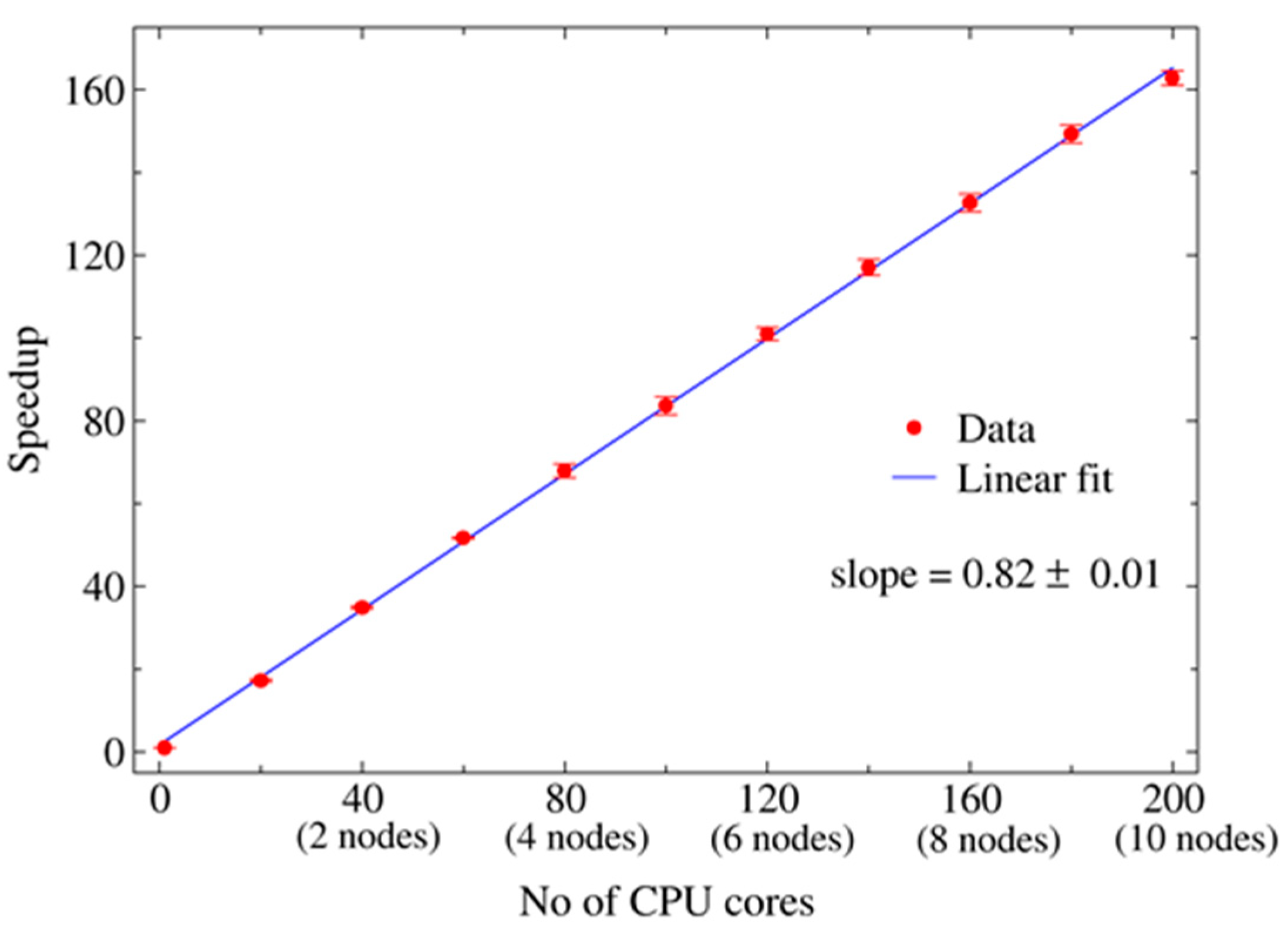
To speed up the calculation of log-likelihood derivatives, we adopted a simple strategy that distributes the workload among multiple processors. Figure 1 illustrates a schematic diagram of the whole process. During the initialization phase of the program, each processor reads in a subset of the training dataset. During each iteration of the gradient descent algorithm, each processor randomly selects a portion of the mini-batch from its own subset of the training dataset and calculates the log-likelihood derivatives. The results of individual processors are summed up to obtain the total log-likelihood derivatives over the complete mini-batch, which are then distributed to all the processors for updating the model parameters. This method leads to a linear speedup, as demonstrated by our test runs performed on Shadow-II as shown in Figure 2 [49,50].

8. Evaluation and Results

Measuring the impact of the RBM and the other machine learning algorithms requires us to handle two important issues. The type of the data that is fed to the algorithms, which we discussed earlier in Section 5, and the tuning of the different hyperparameter setting of the RBM to find the optimal or semi-optimal settings that would lead to the best results when testing the algorithm while at the same time avoiding problems such as overfitting. The hyperparameter settings can differ based on the nature of the application and the characteristics of the data set.

To train the RBM we used the contrastive divergence or the persistent contrastive divergence algorithm. This provides us with the basis to compare the performance of RBM to the other algorithms. We trained and validated our training using two different sets and we kept tuning the hyperparameters using a set of different range of values until we find a set of optimal or semi-optimal parameters. The hyperparameters that were tuned during the training were the learning rate at 0.005, 0.001, 0.05, and 0.01, the number of iterations at 500, 1000, 5000, and 10000, the batch size at 500, 1000, 5000, and 10000, and the k-value at the value of 1 and 10 respectively.

The hyperparameter tuning was done by changing one hyperparameter at a time while keeping all the other settings or hyperparameter values the same. For example, if we chose to change the learning rate then the k-value, the batch size, and the number of iterations should be sustained without any change until we found the learning rate value that produces high or the highest accuracy in that specific setting. This presents us with a solid basis for a rational assessment of the performance of the RBM in various settings, and the weight of each type of the hyperparameters in the learning process. We continued the process of tuning each hyperparameter until we arrived at a point where only minimal fluctuations in learning were identified.

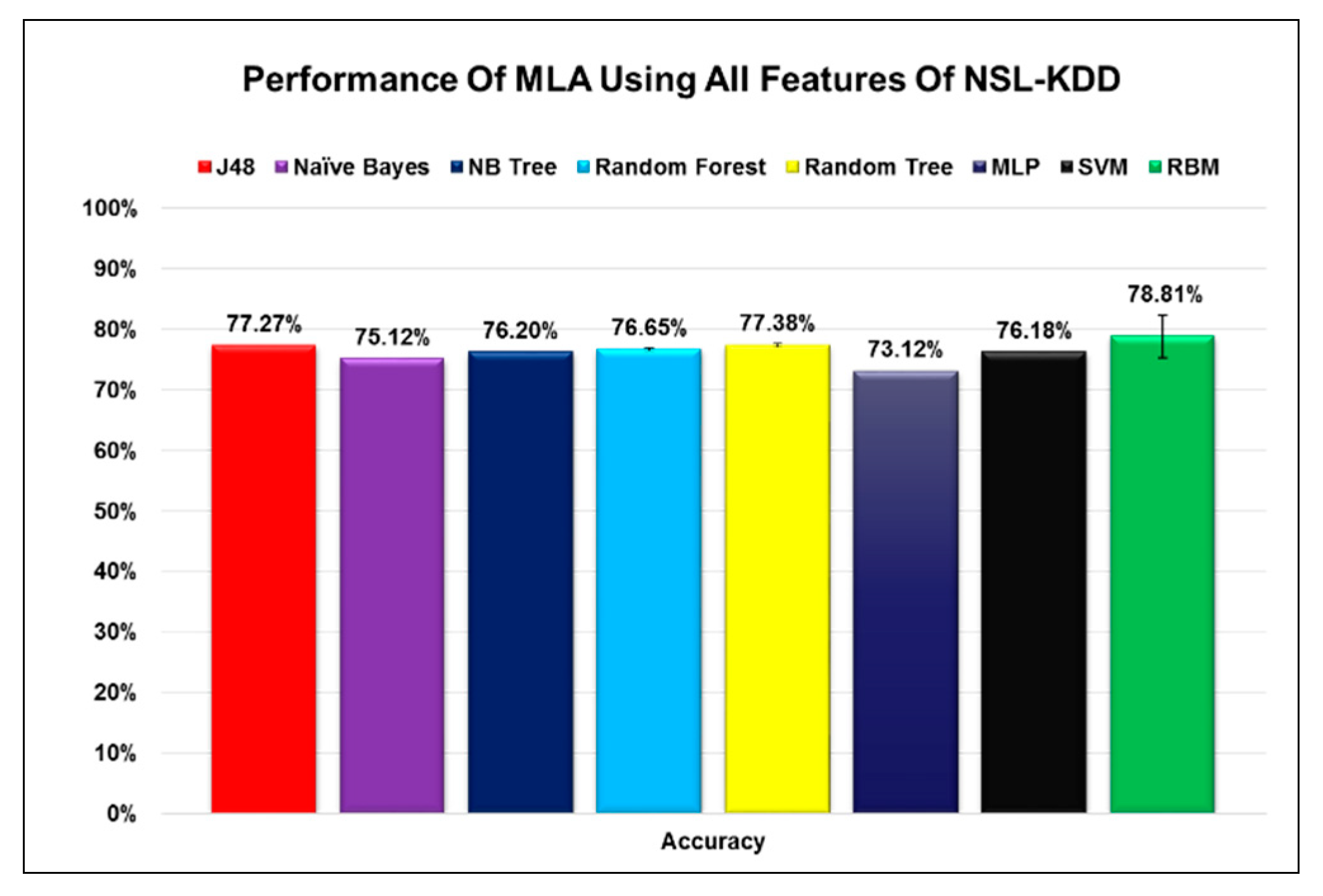
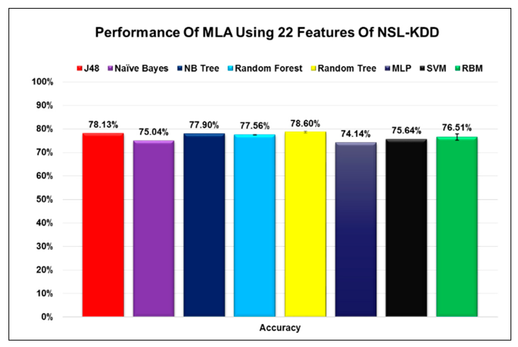
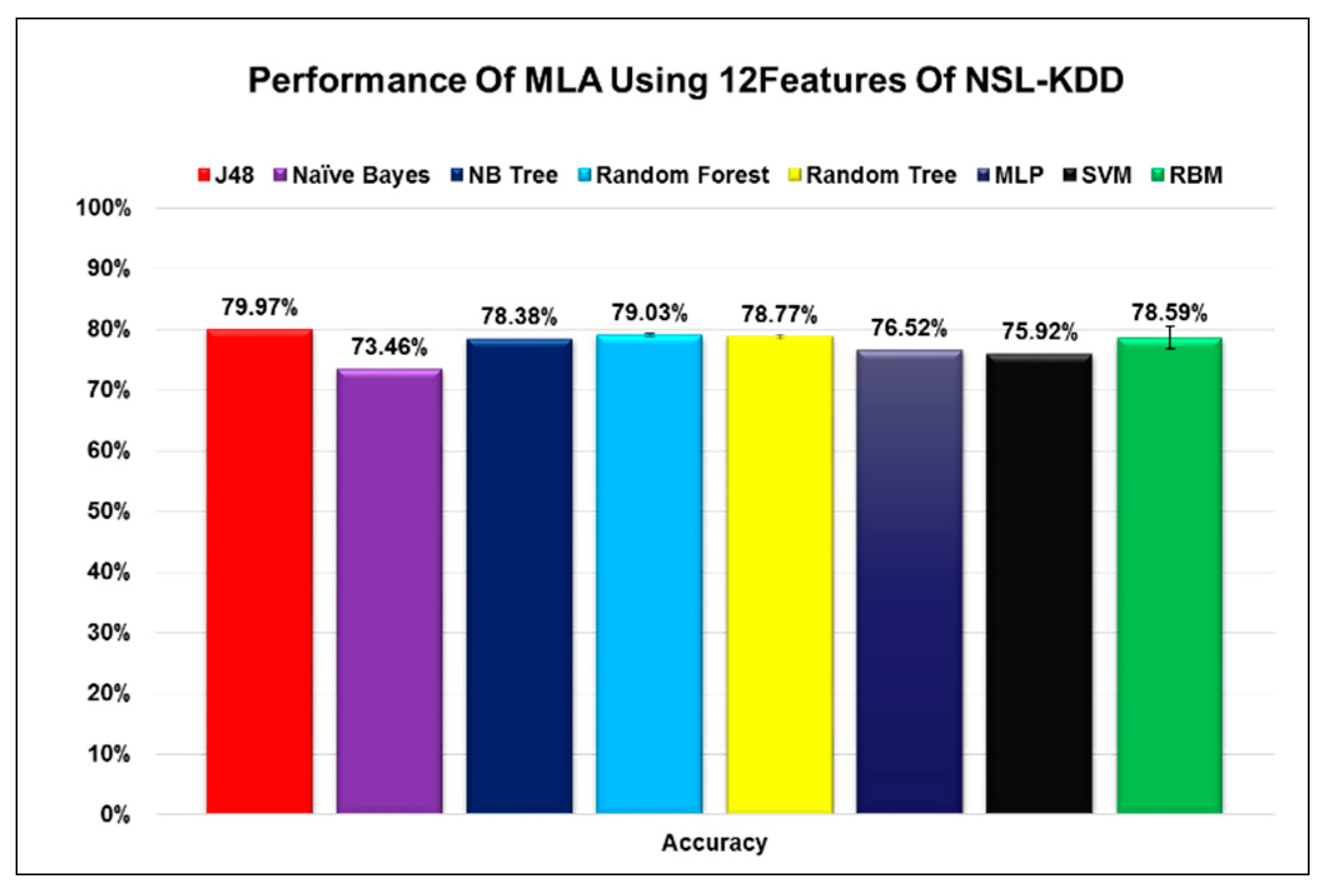
After setting the parameter values for the RBM and evaluating the effectiveness of the RBM training, we assessed the performance of RBM to several popular algorithms used for classification in machine learning. To get a valid assessment between the different algorithms, we trained and tested all the algorithms using the same datasets used for training and testing the RBM. Figure 3, Figure 4 and Figure 5 indicate how the performance of RBM compares against all the other algorithms. It can be seen that the RBM’s performance exceeds some algorithms in many cases and performs very similar to the other algorithms in very specific cases under certain conditions.

An interesting observation regarding the process of selecting different features is that some algorithms performed at their best when all features were selected, while others performed at their best when a smaller number of features was selected. This observation should not be generalized for two reasons. The first reason is that some algorithms like RBM with a probabilistic nature could yield different results at different runs. Especially if we consider that the error margin is within the range of 1-2% when taking the average of different runs. With that in mind, we compared the RBM results for the case when we selected all features to the one when we selected 12 features. An accuracy of 78.81% did not seem that far off from 78.59% with an error margin of 1% to 2%. The second reason for this variation could be attributed to the different ways each algorithm deals with the noise in the data. When we reduced the number of features selected from the data the noise, which is represented by unwanted features that do not contribute to the classification process, will change. Each algorithm handles the noise differently and some algorithms might perform better than others with lesser noise but that is not necessarily a good thing since real-life data will always have noise. Algorithms such as RBM that perform well in both cases might even be better than the algorithms that perform well only when the number of features is reduced since it can handle data even with the presence of noise.

Examining the figures, we could perceive that using the infoGain algorithm during the process of feature selection enabled us to extract the most important features with minimal changes to the accuracy for most algorithms, and in some cases with a slight increase in the accuracy. The change in the accuracy of each algorithm when certain features were selected was below 2% for most of the cases and never exceeded 3%. From our previous analysis, it is obvious that these algorithms can act as a classifier for A-NIDS using the network packet analysis. To get a more in-depth analysis of the suitability of RBM as a model for A-NIDS we refer the reader to our previous research study on the subject [51]. The minor change in accuracy when choosing only a specific number of features can have a drastic effect on the reduction of the size of the datasets as well as the complexity associated with the large number of features especially when we are building machine learning models that act as classifiers for A-NIDS. One more thing we would like to emphasize is the fact that these sets of features do not represent the optimal features to represent the data even though, in theory, they could. More research and studies in this area need to be done to figure out methods and approaches to assess whether those selected features are the best representation of a dataset or if there is even an alternative group of selected features that can give us better results. This alternative solution, if it exists, can even surpass the accuracy of all the features in the dataset since they do not contain any additional unnecessary features and as such can result in higher accuracy.

9. Conclusions

In this paper, we confirmed the effect of appropriate feature selection on the performance of various machine learning algorithms. We used the NSL-KDD a dataset that is used to evaluate the suitability of the algorithms to act as classifiers for an A-NIDS through categorizing the network data into normal and anomalous traffic. In many cases, the selection of the features will result in either an improvement in the accuracy of the classifiers or an insignificant decrease in the accuracy of the classifiers. The change in the accuracy did not exceed 3% for any of the algorithms. This change in accuracy could be attributed to the probabilistic nature of some of those algorithms and their sensitivity to the degree of noise within the data. We also assessed the performance of a RBM when compared to other machine learning algorithms and found that when all features were included in the comparison the RBM surpassed all other classifiers. When the number of features was reduced to 22 and 12, we noticed that the performance of the RBM was on the same level as the majority of other classifiers and that its accuracy was not reduced significantly. We believe that further investigation is essential to attain a solid decision regarding the full effect of feature selection on the performance machine learning algorithms. Future work on the subject will be studying the effect of noise presented in the data on the performance of those algorithms in the context of feature selection to find out which algorithms have more capacity to handle the existence of noise in the data.