Channel-Based Network for Fast Object Detection of 3D LiDAR

Abstract

Currently, there are various methods of LiDAR-based object detection networks. In this paper, we propose a channel-based object detection network using LiDAR channel information. The proposed method is a 2D convolution network with data alignment processing stages including a single-step detection stage. The network consists of a channel internal convolution network, channel external convolution network and detection network. First, the convolutional network within the channel divides the LiDAR data for each channel to find features within the channel. Second, the convolutional network outside the channel combines the LiDAR data divided for each channel to find features between the channels. Finally, the detection network finds objects with the features obtained. We evaluate our proposed network using our 16-channel lidar and popular KITTI dataset. We can confirm that the proposed method detects objects quickly while maintaining performance when compared with the existing network.

1. Introduction

Object detection involves the analysis of input data received through a sensor to identify the locations and classes (pedestrians, dogs, cats, cars, etc.) of an object. The object detection technology is used in many areas, especially in research related to autonomous vehicles. In an autonomous vehicle, object detection looks for objects around the vehicle (other vehicles, pedestrians, obstacles, etc.) for it to drive. Autonomous cars are equipped with multiple sensors for object detection. Among them, sensors that are mostly used for object detection are cameras and Light Detection and Ranging (LiDAR) sensors.

In order to detect objects in the LiDAR, the minimum shape of the object must be visible. Therefore, at least 16 channels of LiDAR data are used for object detection. In general, the higher the channel of a LiDAR, the greater the amount of data and the higher the density, which is more advantageous for object recognition because there are more points expressed on the object.

There are three ways to detect objects using LiDAR data. The first method is to detect objects by discretizing the LiDAR data into specific areas to create voxels. This first method uses voxels, which are 3D data; therefore, less data are lost as a result of changing dimensions. However, it must use a 3D Convolutional Neural Network (CNN). The use of 3D data requires more arithmetic operations than 2D data, making it difficult to use in real time except for a few algorithms. The method is presented in Vote3Deep [1], VoxelNet [2], Vote3D [3], ORION [4], 3D FCN [5], SECOND [6], Rist et al. [7], and PV-RCNN [8]. The second method is to transform LiDAR sensors into top-view (bird’s eye view) images. The top-view method makes data transformation into images and object locating easy.

However, there are disadvantages of increasing the image size depending on the navigation range, and there are many blank spaces on the transformed image, which makes it difficult to recognize the object because of its low data density. In addition, it is challenging to recognize pedestrians, which is a priority for detection. The use of the top-view method is presented in Yu et al. [9], VeloFCN [10], BirdNet [11], Kim et al. [12], Kim et al. [13], PIXOR [14], and BirdNet+ [15]. The third method is to transform data into polar-view (or front-view) images. The polar-view method is more complex than the top-view method but has the advantage of increasing the data density and recognizing pedestrians difficult to detect in the top-view method. Its downside is that objects often overlap because images change on an angle basis, and, in the case of overlaps, the data at the back are disregarded, resulting in data loss. The use of the polar-view method is presented in LiSeg [16], Kwon et al. [17], and Lee et al. [18]. In some cases, a mixture of the second and third methods is used. MV3D [19] is a typical case of such a mixed use.

This paper proposes a new network method that is different from those above. (1) LiDAR has a fixed number of channels. Points on the same channel are separated by distance but are continuous when viewed by a channel. Using the continuous properties, features within the channel are extracted. (2) Looking at the LiDAR data in the form of a matrix, it can be said that the channel data are also continuous. Therefore, to obtain the feature of channel data, the results from each Channel Internal Convolution Network are combined and the feature is extracted through Channel External Convolution Network (3) The class and location of an object are identified through the detection network.

This paper makes the following contributions: First, we propose an object detection network based on a LiDAR channel. LiDAR data adversely affect convolution due to the large amount of empty space when searching a wide range from a limited number of points based on distance. When using the channel-based method, since the LiDAR data is sorted, the empty space of the data can be eliminated. Second, using the channel-based method, the actual LiDAR data is 3D, but since it can be used like 2D data, the speed of the network is increased by using the 2D convolution method instead of the 3D convolution.

This paper is organized as follows: Section 2 provides an overview of the existing networks, Section 3 proposes a new network, Section 4 demonstrates the excellence of the proposed network through experiments, and Section 5 provides conclusions.

2. Related Work

2.1. Voxel-Based Network

A voxel is a volume element, representing a value on a regular grid in a three-dimensional space. The number of grids $H^{\prime }$, $W^{\prime }$ and $D^{\prime }$ that occurs when the size of the voxels to be used in 3D space $H\times W\times D$ to detect an object are $h_v$, $w_v$, $d_v$ is as follows:

$$H^{\prime }=\frac{H}{h_v}, W^{\prime }=\frac{W}{w_v}, D^{\prime }=\frac{D}{d_v}$$

(1)

Input data that goes into the network through random sampling using voxels are created. Next, data features are extracted by applying 3D convolutions. Finally, the class and location of an object recognized using RPN is identified. Figure 1 summarizes the voxel-based network structure.

Figure 1. Network structure based on voxel.

2.2. Image Transformation-Based Network

The image transformation-based network concerns a method of recognizing objects by transforming them into 2D images using 3D LiDAR data. When transforming LiDAR data into images, the top- and polar-view methods are generally used. The equations for transforming the top [12] and polar views [17] are as follows:

$$k_t={\displaystyle ⎣}\left(x_{i,j}+R_x\right)\times \frac{M}{2R_x}{\displaystyle ⎦}$$

(2)

$$l_t={\displaystyle ⎣}\left(y_{i,j}-R_y\right)\times \frac{-N}{2R_y}{\displaystyle ⎦}$$

(3)

$$k_p={\displaystyle ⎣}\frac{\mathrm{atan}2\left(y_{i,j}, x_{i,j}\right)}{\alpha }{\displaystyle ⎦}$$

(4)

$$l_p={\displaystyle ⎣}\frac{{\sin }^{-1}{z}_{i,j}/\sqrt{x_{i,j}^2+y_{i,j}^2+z_{i,j}^2}}{\beta }{\displaystyle ⎦}$$

(5)

Equations (2) and (3) are the transformation equations for the top-view method while Equations (4) and (5) are for the polar-view method. $\left(k, l\right)$ are the pixel coordinates whose image sizes are $M$ and $N$, and $R_x$, $R_y$ are the values of $x$ and $y$ axes of the largest LiDAR to be measured. Finally, $\alpha$ and $\beta$ are the constant that determines the image size in the polar view. Figure 2 summarizes the image transformation-based network structure.

Figure 2. Network structure based on image transformation.

3. LiDAR Channel-Based Network

The structure of the network proposed in this paper is shown in Figure 3. It is summarized as follows: first, the features of each channel are extracted through the channel’s internal convolution network after divide the LiDAR data by channel. Second, the data are combined to obtain the features of the data of each channel through its external convolution network. Third, the presence of objects is verified through the detection network. Fourth and lastly, the class of the object is obtained in the class layer, and the bounding box of the object is obtained in the box layer.

Figure 3. The structure of the proposed network.

3.1. Channel Internal Convolution Network

The output of point cloud $L \left(L=\left\{p_{i,j}\right\}, p_{i,j}=\left\{x_{i,j}, y_{i,j}, z_{i,j},I_{i,j}\right\}\right)$, which is the data given in LiDAR sensors, is shown in Figure 4a,b if the given point clouds are arranged by channel. We want to define the “channel” of the LiDAR. For example, Velodyne HDL-64E has 64 channels ($C_1$-$C_{64}$). Points in the same channel can be displayed in one column. It is summarized in Equations (6) and (7):

$$L=\left[\begin{array}{c}\begin{array}{c}{C}_1\\ C_2\end{array}\\ \begin{array}{c}⋮\\ C_i\end{array}\end{array}\right]$$

(6)

$$C_i=\left[\begin{array}{cc}{p}_{i,1}& p_{i,2}\end{array}\begin{array}{cc}\cdots & p_{i,j}\end{array}\right]$$

(7)

where $L$ is the whole LiDAR data, and $C_i$ represents a set of points belonging to the channel. $p_{i,j}$ represents a point, and $j$ is an index on each channel. Each point $\left(p_{i,j}\right)$ contains locations $\left(x, y, z\right)$ and reflection $\left(I\right)$values.

Figure 4. How to display point cloud data: (a) output data, (b) alignment data.

The advantage of sorting LiDAR data by channel is that the density of the data increases. Sorting the lidar data by channel increases the density of the data, which is advantageous for object recognition. Due to the sorted data, it can be viewed in the form of an image with a depth of 4($\mathrm{x},\mathrm{y},\mathrm{z},\mathrm{I}$). If you can see it in the form of an image, you can use 2D CNN instead of 3D CNN. 2D convolution used in 2D CNN can be expressed as follows.

$$D_2={\displaystyle \sum }{\displaystyle \sum }f\left(x,y\right)g\left(a-x\right)\left(a-y\right)$$

(8)

The number of operations varies depending on the size ($i, j$) of the pixel and the size of the filter, but the number of 2D convolutions used in 2D CNN can be expressed as Equation (9).

$$TOTA{L}_2=n_2\left(W^{\prime }-f_2^x\right)\left(H^{\prime }-f_2^y\right)$$

(9)

$n_2$ is the number of convolutions, and $f_2^{*}$ is the size of the filter in each direction.

Runtime can be reduced because the operation time of 2D Convolution is shorter than 3D Convolution and there is a difference in the number of Convolutions.

The reason for separating the LiDAR channel is that, in the case of a rider capable of 360° scanning, the points on the same channel have many similarities. For example, when you scan a flat surface, the distance and reflection values of LiDAR data on the same channel are similar. However, if an object is present, the distance or the reflection values are different in the middle, as shown in Figure 4a. Therefore, data are discretized by channel to apply it to the algorithms proposed in this paper because the data of each channel are interrelated. Convolutions inside the channel are performed using the divide channel data.

We use the channel data separated based on the equation to perform convolution inside the channel. Each channel’s internal convolution network consists of 12 convolution layers and 4 pooling layers, and the overall numbers are presented as $12\times i$ convolution layers and $4\times i$ pooling layers. We used ReLU as the active function after convolution. The size of the convolution mask on the convolution layer is $1\times 3$. Convolutions apply to the $x$, $y$, $z$, and $I$ values of the LiDAR data on each LiDAR channel. A set comprising of three convolutions and one pooling is repeated four times. The results of the channel’s internal convolution network produce a feature map (${\overline{F}}_i$) for each channel.

3.2. Channel External Convolution Network

Although the previous section mentions that the data of each channel is important, Figure 5 shows that data between channels are as relevant as the data of each channel. The purpose of the channel’s external convolution network is to extract channel-specific and channel-to-channel features of the data.

Figure 5. Configuration of a channel internal convolution network.

The channel’s external convolution network consists of three convolution layers, as shown in Figure 6. The size $3\times 3$ is used for the convolution layer’s mask. At the end of the network, a new feature map ($F^{″}$) [20] is created by connecting the feature map ($F^{\prime }$) that resulted from convolutions and the feature map ($F$) that was used as input. For the input data for the channel’s external convolution, F that combines the results of the previous section (${\overline{F}}_1, {\overline{F}}_2, \cdots , {\overline{F}}_i$) is used. The output data are $F^{″}$, and its feature map is in the same size as that of $F$.

Figure 6. Configuration of a channel external convolution network.

3.3. Detection Network

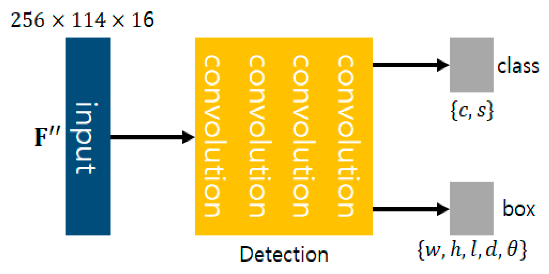
A detection network is a network that determines whether an object is present or not by using $F^{″}$ as input, which is the result of a channel’s external convolution network. For the structure of the detection network, refer to the structure of the header network of PIXOR [14]. A detection network has four convolution layers and uses a mask sized $3\times 3$. We used ReLU as the active function after convolution. The final data obtained after four convolution layers are used as input for the class and box layers.

The class layer is outputs 2-channel feature map and configured to output classes and scores $\left(c, s\right)$ for an object concerned. The box layer is outputs 5-channel feature map and configured to display the position of the object, the size of the box, and the angle $\left(h, w, l, d, \theta \right)$ of the object. The detection network is illustrated in Figure 7.

Figure 7. Configuration of a detection network.

3.4. Loss Function

The loss function is a function that defines how well a network deals with training data. In general, the learning objective of a network is to minimize the value of the loss function. The proposed network’s loss function is as follows:

$$E_{total}=E_{class}+E_{box}$$

(10)

where $E_{total}$ represents the loss function of the entire network, $E_{class}$ is the loss function of a class layer, and $E_{box}$ is the loss function of a box layer. The function in each loss function uses the cross-entropy [21], and the equation is as follows. E equals the output when the error $t_k$ is the ground truth (GT) value and $y_k$ is the output of the network.

$$E=-{\displaystyle \sum }{t}_k\log y_k$$

(11)

The entire network goes through the learning process using the above loss function in the end-to-end method with Adam optimization [22].

4. Experiment

This section evaluates the performance of the proposed algorithm. The experiment carried out is as follows: First, the existing object-detection algorithms are compared to the proposed algorithm using the 16-channel LiDAR. Second, the existing object-detection algorithms are compared to the proposed algorithm using the KITTI dataset [23] (64-channel LiDAR).

4.1. Experiment Setup

4.1.1. Object Detection Test Using 16-Channel LiDAR

LiDAR used in the experiment is Velodyne VLP-16, and it is fitted to the vehicle shown in Figure 8. The operating system for the personal computer (PC) is Ubuntu. The experiment was conducted in the ROS Kinetic environment, the central processing unit was i5-6600 (3.30 GHz), and the graphics processing unit used was GeForce GTX 1080 ti. The data obtained while driving the vehicle around the campus was used for the experiment. We trained the algorithm using 2276 frames of training data and 1138 frames of test data.

Figure 8. Configuration of a detection network.

The object detection results were compared using existing algorithms (the voxel, top-view, and polar-view methods) and the proposed network. Studies [2,12,17] were used for the voxel, top-view, and polar-view methods, respectively. Lastly, [19] was used for a mixture of two or more methods for comparisons.

4.1.2. Object Detection Test Using 64-Channel LiDAR

The KITTI datasets [23] were used for the experiment of the 64-channel LiDAR. The LiDAR sensor used in the KITTI datasets is Velodyne HDL-64E. In the experiment results, two classes (vehicle, pedestrian) represent the results of the KITTI benchmark. The runtime test results used the PC used in Section 4.1.1.

4.2. Experiment Result

4.2.1. Object Detection Test Using 16-Channel LiDAR

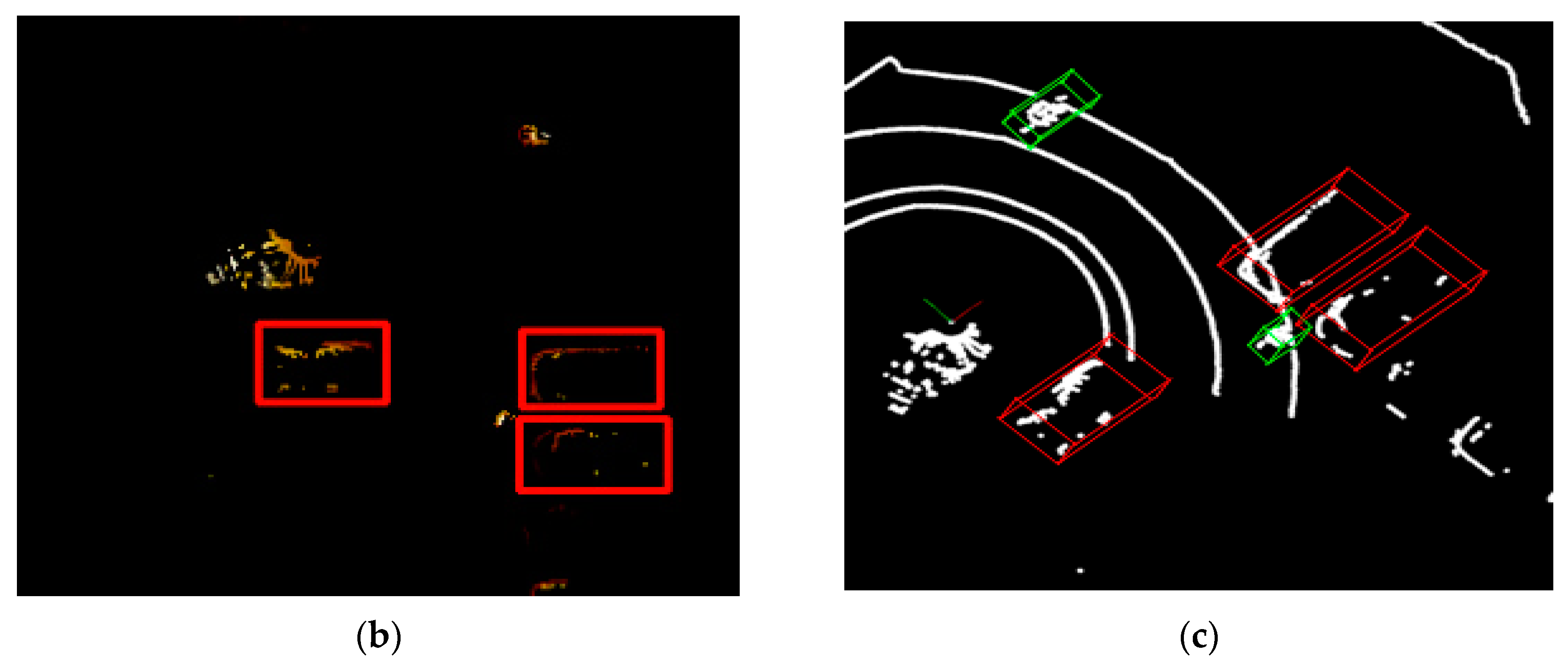
The experiment results are shown in Table 1. We can confirm that the proposed method is faster in runtime than the existing method. The reason was explained in the previous section, but the convolution operation was reduced and the time was faster. Additionally, the results of the vehicle recognition were small, but it was confirmed that the results of pedestrians were different. Due to the low density of the LiDAR data, there are many empty spaces, and because of the small percentage of pedestrians, we believe that the voxels with pedestrians are few and have low performance. The relatively dense polar-view transformation method and the proposed method are found to have a higher performance than the voxel method. However, in some circumstances, the polar view was unable to detect the object. The top-view transformation method is excluded because it cannot detect pedestrians. Figure 9 illustrates the results of object detection in some networks used in the experiment.

Table 1. Results of 16-channel LiDAR object detection.

	Type	Vehicle			Pedestrian			Run Time
		Precision	Recall	F1	Precision	Recall	F1
VoxelNet [2]	Voxel	83.51 %	77.73 %	80.52 %	60.67 %	43.24 %	50.49 %	46 ms
Kim et al. [12]	Top	83.17 %	80.58 %	81.85 %	-	-	-	41 ms
Kwon et al. [17]	Polar	87.32 %	81.52 %	84.32 %	80.72 %	76.87 %	78.75 %	42 ms
MV3D [19]	Top,front	79.23 %	50.75 %	61.87 %	-	-	-	240 ms
proposed	channel	86.81 %	80.16 %	83.35 %	78.33 %	72.87 %	75.50 %	21 ms

Figure 9. Results of the 16-channel lidar object detection: (a) polar-view, (b) top-view, (c) proposed methods; Vehicle is red, pedestrian is green.

4.2.2. Object Detection Test Using 64-Channel LiDAR

Table 2 shows the KITTI benchmark results. The “Type” is the method used on the network. The KITTI benchmark experiment was conducted on two classes: vehicle and pedestrian. First, in the case of a vehicle, the proposed network shows the average performance among the networks in Table 2. In detail, it has higher performance than the top-view method and lower than the voxel method Next, in the case of pedestrians, the proposed network also showed average performance.

Table 2. Results of KITTI benchmark (3D Object Detection).

	Type	Vehicle			Pedestrian			Run Time *
		Easy	Moderate	Hard	Easy	Moderate	Hard
VoxelNet [2]	Voxel	77.47 %	65.11 %	57.73 %	39.48 %	33.69 %	31.51 %	50 ms
PV-RCNN [8]	Voxel	90.25 %	81.43 %	76.82 %	52.17 %	43.29 %	40.29 %	83 ms
MV3D [19]	Top,front	74.97 %	63.63 %	54.00 %	-	-	-	254 ms
F-PointNet [24]	RGB,front	82.19 %	69.79 %	60.59 %	50.53 %	42.15 %	38.08 %	186 ms
BirdNet+ [15]	Top-view	70.14 %	51.85 %	50.03 %	37.99 %	31.46 %	29.46 %	110 ms
PointRCNN [25]	point	86.96 %	75.64 %	70.70 %	47.98 %	39.37 %	36.01 %	107 ms
3DSSD [26]	point	88.36 %	79.57 %	74.55 %	54.64 %	44.27 %	40.23 %	41 ms
proposed	channel	86.40 %	77.74 %	72.97 %	47.14 %	39.72 %	37.25 %	32 ms

* Runtime is the result of self-testing with the PC used in Section 4.1.1.

The runtime experiment was conducted with the PC in Section 4.1.1. As expected, the data transformation method has a longer runtime in the transformation process, but we can confirm that the method we proposed is the shortest.

5. Conclusions

In this paper, we proposed a new method called object detection network based on a LiDAR channel. The LiDAR data were aligned in a matrix to eliminate the empty space of the data. Features were extracted from each channel of the lidar using Channel Internal Convolution Network. The Channel External Convolution Network was used to extract the features of the LiDAR channel data. Finally, the class and box of the object were detected using the two features previously obtained from the detection network.

Instead of 3D convolution with a lot of computation, 2D convolution was used to reduce computation. The experimental results showed that the proposed network has medium performance in terms of classification accuracy, but has higher performance in terms of runtime.

References

- Engelcke, M.; Rao, D.; Wang, D.Z.; Tong, C.H.; Posner, I. Vote3Deep: Fast object detection in 3D point clouds using efficient convolutional neural networks. In Proceedings of the 2017 IEEE International Conference on Robotics and Automation, Singapore, 29 May–3 June 2017; pp. 1356–1361. [Google Scholar]
- Zhou, Y.; Tuzel, O. VoxelNet: End-to-End learning for point cloud based 3D object detection. In Proceedings of the 2018 IEEE Conference on Computer Vision and Pattern Recognition, Salt Lake City, UT, USA, 18–23 June 2018; pp. 4490–4499. [Google Scholar]
- Wang, D.Z.; Posner, I. Voting for voting in online point cloud object detection. In Proceedings of the Robotics: Science and Systems, Rome, Italy, 13–17 July 2015; Volume 1. [Google Scholar]
- Sedaghat, N.; Zolfaghari, M.; Amiri, E.; Brox, T. Orientation-boosted voxel nets for 3D object recognition. In Proceedings of the 28th British Machine Vision Conference, London, UK, 4–7 September 2017. [Google Scholar]
- Li, B. 3D fully convolutional network for vehicle detection in point cloud. In Proceedings of the 2017 IEEE/RSJ International Conference on Intelligent Robots and Systems, Vancouver, BC, Canada, 24–28 September 2017; pp. 1513–1518. [Google Scholar]
- Yan, Y.; Mao, Y.; Li, B. SECOND: Sparsely Embedded Convolutional Detection. Sensors 2018, 18, 3337. [Google Scholar] [CrossRef]
- Rist, C.B.; Enzweilrt, M.; Gavrila, D.M. Cross-Sensor Deep Domain Adaptation for LiDAR Detection and Segmentation. In Proceedings of the 2019 IEEE Intelligent Vehicles Symposium, Paris, France, 9–12 June 2019; pp. 1535–1542. [Google Scholar]
- Shi, S.; Guo, C.; Jiang, L.; Wang, Z.; Shi, J.; Wang, X.; Li, H. PV-RCNN: Point-Voxel Feature Set Abstraction for 3D Object Detection. arXiv 2019, arXiv:1912.13192. [Google Scholar]
- Yu, S.; Westfechtel, T.; Hamada, R.; Ohno, K.; Tadokoro, S. Vehicle Detection and Localization on Bird’s Eye View Elevation Images Using Convolutional Neural Network. In Proceedings of the 2017 IEEE International Symposium on Safety, Security and Rescue Robotics, Shanghai, China, 11–13 October 2017; pp. 102–109. [Google Scholar]
- Li, B.; Zhang, T.; Xia, T. Vehicle detection from 3D lidar using fully convolutional network. In Proceedings of the 2016 Robotics: Science and Systems Conference, Ann Arbor, MI, USA, 18–22 June 2016. [Google Scholar]
- Beltran, J.; Guindel, C.; Moreno, F.M.; Cruzado, D.; Garcia, F.; Escalera, A. BirdNet: A 3D object detection framework from LiDAR information. arXiv 2018, arXiv:1805.01195. [Google Scholar]
- Kim, T.H.; Kwon, S.S.; Lee, K.S.; Park, T.H. Multiple lidars calibration and deep learning based vehicle recognition. In Proceedings of the 2017 KSAE Annual Spring Conference, Jeju, Korea, 18–20 May 2017; pp. 1356–1357. [Google Scholar]
- Kim, Y.; Kim, J.; Koh, J.; Choi, J.W. Enhanced Object Detection in Bird’s Eye View Using 3D Global Context Inferred from Lidar Point Data. In Proceedings of the 2019 IEEE Intelligent Vehicles Symposium, Paris, France, 9–12 June 2019; pp. 2516–2521. [Google Scholar]
- Yang, B.; Luo, W.; Urtasun, R. PIXOR: Real-Time 3D Object Detection from Point Clouds. In Proceedings of the 2018 IEEE/CVF Conference on Computer Vision and Pattern Recognition, Salt Lake City, UT, USA, 27–30 June 2016; pp. 7652–7660. [Google Scholar]
- Barrera, A.; Guindel, C.; Beltrán, J.; García, F. BirdNet+: End-to-End 3D Object Detection in LiDAR Bird’s Eye View. arXiv 2020, arXiv:2003.04188. [Google Scholar]
- Zhang, W.; Zhou, C.; Yang, J.; Huang, K. LiSeg: Lightweight road-object semantic segmentation in 3D LiDAR scans for autonomous driving. In Proceedings of the 2017 IEEE Conference on Computer Vision and Pattern Recognition, Changshu, China, 26–30 June 2018; pp. 1021–1026. [Google Scholar]
- Kwon, S.S.; Park, T.H. Polar-View Based Object Detection Algorithm Using 3D Low-Channel Lidar. J. Inst. Control Robot. Syst. 2019, 25, 56–62. [Google Scholar] [CrossRef]
- Lee, J.S.; Jo, J.H.; Park, T.H. Segmentation of Vehicles and Roads by a Low-Channel Lidar. IEEE Trans. Intell. Transp. Syst. 2019, 20, 4251–4256. [Google Scholar] [CrossRef]
- Chen, X.; Ma, H.; Wan, J.; Li, B.; Xia, T. Multi-view 3D object detection network for autonomous driving. In Proceedings of the 2018 IEEE Intelligent Vehicles Symposium, Honolulu, HI, USA, 21–26 July 2017; pp. 6526–6534. [Google Scholar]
- He, K.; Zhang, X.; Ren, S.; Sun, J. Deep Residual Learning for Image Recognition. In Proceedings of the 2016 IEEE Conference on Computer Vision and Pattern Recognition, Las Vegas, NV, USA, 18–23 June 2018; pp. 770–778. [Google Scholar]
- Boer, P.T.; Kroese, D.P.; Mannor, S.; Rubinstein, R.Y. A Tutorial on the Cross-Entropy Method. Ann. Oper. Res. 2005, 1, 56–62. [Google Scholar]
- Kingma, D.P.; Ba, J.L. Adam: A Method for Stochastic Optimization. arXiv 2014, arXiv:1412.6980. [Google Scholar]
- Geiger, A.; Lenz, P.; Urtasun, R. Are we ready for autonomous driving? The kitti vision benchmark suite. In Proceedings of the 2012 IEEE Conference on Computer Vision and Pattern Recognition, Providence, RI, USA, 16–21 June 2012; pp. 3354–3361. [Google Scholar]
- Qi, C.R.; Liu, W.; Wu, C.; Su, H.; Guibas, L.J. Frustum PointNets for 3D Object Detection from RGB-D Data. arXiv 2017, arXiv:1711.08488. [Google Scholar]
- Shi, S.; Wang, X.; Li, H. PointRCNN: 3D Object Proposal Generation and Detection from Point Cloud. In Proceedings of the 2019 IEEE/CVF Conference on Computer Vision and Pattern Recognition, Long Beach, CA, USA, 15–20 June 2019; pp. 770–779. [Google Scholar]
- Yang, Z.; Sun, Y.; Liu, S.; Jia, J. 3DSSD: Point-based 3D Single Stage Object Detector. arXiv 2020, arXiv:2002.10187. [Google Scholar]
© 2020 by the authors. Licensee MDPI, Basel, Switzerland. This article is an open access article distributed under the terms and conditions of the Creative Commons Attribution (CC BY) license (http://creativecommons.org/licenses/by/4.0/).