UAV Autonomous Aerial Combat Maneuver Strategy Generation with Observation Error Based on State-Adversarial Deep Deterministic Policy Gradient and Inverse Reinforcement Learning

Abstract

With the development of unmanned aerial vehicle (UAV) and artificial intelligence (AI) technology, Intelligent UAV will be widely used in future autonomous aerial combat. Previous researches on autonomous aerial combat within visual range (WVR) have limitations due to simplifying assumptions, limited robustness, and ignoring sensor errors. In this paper, in order to consider the error of the aircraft sensors, we model the aerial combat WVR as a state-adversarial Markov decision process (SA-MDP), which introduce the small adversarial perturbations on state observations and these perturbations do not alter the environment directly, but can mislead the agent into making suboptimal decisions. Meanwhile, we propose a novel autonomous aerial combat maneuver strategy generation algorithm with high-performance and high-robustness based on state-adversarial deep deterministic policy gradient algorithm (SA-DDPG), which add a robustness regularizers related to an upper bound on performance loss at the actor-network. At the same time, a reward shaping method based on maximum entropy (MaxEnt) inverse reinforcement learning algorithm (IRL) is proposed to improve the aerial combat strategy generation algorithm’s efficiency. Finally, the efficiency of the aerial combat strategy generation algorithm and the performance and robustness of the resulting aerial combat strategy is verified by simulation experiments. Our main contributions are three-fold. First, to introduce the observation errors of UAV, we are modeling air combat as SA-MDP. Second, to make the strategy network of air combat maneuver more robust in the presence of observation errors, we introduce regularizers into the policy gradient. Third, to solve the problem that air combat’s reward function is too sparse, we use MaxEnt IRL to design a shaping reward to accelerate the convergence of SA-DDPG.

1. Introduction

Compared with human-crewed aircraft, military UAVs have attracted much attention for their low cost, long flight time, and fearless sacrifice [1]. With the development of sensor technology, computer technology, and artificial intelligence technology, the operational performance of military UAVs has been significantly improved, and the range of tasks that can be performed has been continuously expanded. Although military UAVs can perform reconnaissance and ground attack missions, most control decisions are made by ground station controllers. Because it is difficult to adapt to the fast and changeable air battle scene, the traditional ground station command operation is difficult to command the UAV for aerial combat [2]. Moreover, since the weapons and sensors mounted by UAVs are less than the human-crewed aircraft, compared with the aerial combat of the human-crewed aircraft, UAVs should be fought in the close range. Therefore, the autonomous aerial combat of UAVs in close range is an important research topic.

This study focuses on gun-based aerial combat WVR, referred to as dogfighting. Although missiles have developed into major equipment for beyond-visual-range operations, particularly for second-generation fighters and later [3], their effectiveness and death toll have been lower than expected. Therefore, as the next-generation fighter, unmanned combat with guns is considered the key to WVR combat.

Since the early 1960s, a great deal of research has been done on autonomous aerial combat, and some remarkable research results have been published. The problem of aerial combat is modeled as pursuit-evasion games [4,5,6], and various theoretical and optimal control schemes provide solutions for autonomous aerial combat. Using differential game theory [7], the aerial combat model is modeled as a deterministic, complete information pursuer-evader game model. In Reference [8], approximate dynamic programming (ADP), a real-time autonomous one-to-one aerial combat method, was studied, and the results were tested in real-time indoor autonomous vehicle test environments (RAVEN). ADP differs from classical dynamic programming in that it constructs a continuous function to approximate future returns. ADP does not need to perform future reward calculations for each discrete state. Therefore, its real-time performance is reliable. A more complex two-on-one combat was treated as a differential game in three-dimensional space [9]. These theoretical approaches make possible the mathematical interpretation of the problem of aerial combat. However, they may include oversimplified assumptions, such as fixed roles or two-dimensional motion, to reduce complexity and computational time.

Some approaches are to model autonomous aerial combat as rule-based heuristic systems that imitate the behavior of human pilots. In Reference [10,11,12], the maneuvering library design, control application, and maneuvering identification based on the basic fighter maneuvers (BFM) expert system are presented. Based on a combination of the BFM library, target prediction, and impact point calculations, an autonomous aerial combat framework for two-on-two engagements was proposed in [9]. At the same time, the influence graph model is used to model the pilot’s decision-making process choosing the right maneuver at every moment in the aerial combat [13,14]. The rule-based system produces real and reasonable simulation results. However, it is difficult to deal with all combat situations, modify previously designed rules, and add new rules.

Artificial neural network and reinforcement learning methods have recently exhibited an improved performance by generating effective new tactics for various simulation environments. Based on the artificial neural network, aerial combat maneuver decision-making is learned from a large number of aerial combat samples with strong robustness [15,16,17,18]. However, aerial combat samples need to include multiple groups of time series and aerial combat results. Due to the difficulty in obtaining samples for aerial combat, it is necessary to mark samples at each sampling time manually. Therefore, aerial combat samples’ problem limits the application of the method of generating an aerial combat maneuver strategy based on a neural network. In Reference [19], an algorithm based on DDPG and a new training method was proposed to reduce training time and simultaneously obtain sub-optimal but effective training results. A discrete action space was used, and the aerial combat maneuvering decisions of an opponent aircraft were considered. However, the current reinforcement learning methods all consider that the acquired aerial combat status is accurate, which is inconsistent with the real aerial combat. In addition, reinforcement learning has also been applied in the fields of UAV flight control and multi UAVs cooperative flight control [20,21,22]. In Reference [20], deep Q-network, policy gradient and DDPG are used to design the 2-DOF flight attitude simulator control system and the feasibility of model-free reinforcement learning algorithm is proved through the experimental results. In Reference [21], the output reference model tracking control for a nonlinear real-world two-inputs–two-outputs aerodynamic system is solved by iterative model-free approximate value iteration (IMF-AVI), and theoretical analysis shows convergence of the IMF-AVI while accounting for approximation errors and explains for the robust learning convergence of the NN-based IMF-AVI. In Reference [22], a UAV control policy based on DDPG to address the combination problem of 3-D mobility of multiple UAVs and energy replenishment scheduling, which ensures energy efficient and fair coverage of each user in a large region and maintains the persistent service.

Further practical improvements are required for the WVR autonomous aerial combat. We propose a novel the autonomous aerial combat maneuver strategy generation algorithm with high-performance and high-robustness based on the SA-DDPG algorithm. In order to consider the error of the aircraft sensors, we model the aerial combat WVR as a state-adversarial Markov decision process (SA-MDP), which introduce the small adversarial perturbations on state observations and these perturbations do not alter the environment directly, but can mislead the agent into making suboptimal decisions. SA-DDPG introduce a robustness regularizers related to an upper bound on performance loss at the actor-network to improve the robustness of the aerial combat strategy. At the same time, a reward shaping method based on MaxEnt IRL is proposed to improve the efficiency of the aerial combat strategy generation algorithm. Finally, the aerial combat strategy generation algorithm’s efficiency and the performance and robustness of the resulting aerial combat strategy are verified by simulation experiments. Our contribution in this paper is a novel autonomous aerial combat maneuver strategy generation algorithm with high-performance and high-robustness based on SA-DDG. Unlike existing methods, the observation errors of UAV is introduced into the air combat model, and regularizer is introduced into the policy gradient to make the strategy network of air combat maneuver more robust. Finally, to solve the problem that air combat’s reward function is too sparse, we use MaxEnt IRL to design a shaping reward to accelerate the convergence of SA-DDPG.

The remainder of this paper is organized as follows. Section 2 explains and defines the aerial combat model based on SA-MDP. Next, the specific theory and techniques for autonomous aerial combat maneuver strategy generation based on SA-DDPG are described in Section 3. A reward shaping method based on MaxEnt IRL is proposed in Section 4. Section 5 details the virtual combat environment and analyzes the performance of the proposed algorithm. This paper is concluded in Section 6. In this study, the UAV piloted by the proposed algorithm, and the target is referred to as the attacker and the target, respectively, for simplicity.

2. Aerial Combat Modeling

2.1. State-Adversarial Markov Decision Process (SA-MDP)

Markov decision process (MDP) is widely used in robotics, economics, manufacturing, and automatic control [23]. MDP is a mathematical framework for probabilistic modeling of the interactions between agents and the environment [24]. Agent is assumed to be learner or decision-maker, interacting with the environment. It receives a reward and a representation of the environment’s state at each time step and imposes an action on the environment that may change its future state. This interaction between the agent and the environment is shown in Figure 1a.

A typical MDP is represented using a 6-tuple $(\mathcal{S},\mathcal{A},\mathcal{T},\gamma ,\mathcal{D},\mathcal{R})$, where $\mathcal{S}=\{s_0,s_1,\dots ,s_n\}$ is a set of possible states that represent a dynamic environment, $\mathcal{A}=\{a_0,a_1,\dots ,a_n\}$ is a set of available actions that the agent can select at a certain state, $\mathcal{T}$ is the state transition function which is determined by the current state and the next action of the agent. MDP assumes that performing an operation in a given state depends only on the current state-action pair, not on the previous states and actions, that is,

$$\mathbb{P}\left(s_{t+1}|s_t,a_t,s_{t-1},a_{t-1},\dots ,s_0,a_0\right)=\mathbb{P}\left(s_{t+1}|s_t,a_t\right)$$

(1)

Equation (1) is called Markov property [25]. So, its mapping relationship is shown in Equation (2).

$$\mathcal{T}:\mathcal{S}\times \mathcal{A}\times {\mathcal{S}}^{\prime }\to [0,1]$$

(2)

$\mathcal{T}$ is the state transition probability matrix that provides the probability of the system transition between every pair of the states, $\gamma \in [0,1)$ is the discount rate that guarantees the convergence of total returns. $\mathcal{D}$ is the initial state distribution, and $\mathcal{R}$ is the reward function, which specifies the reward for taking action in a state whose mapping relationship is shown in Equation (3).

$$\mathcal{R}:\mathcal{S}\times \mathcal{A}\to \mathbb{R}$$

(3)

The core objective of an MDP is to find a policy $\pi$ for the agent, where the policy $\pi :\mathcal{S}\to \mathcal{A}$ specifies the action to take at the current state, where $\pi \left(s\right)=a$ denotes that action a is always executed in-state s following the policy $\pi$. Moreover, the goal is to find the optimal policy of ${\pi }^{*}$ that maximizes the cumulative discounted reward over an infinite horizon:

$${\pi }^{*}=arg\underset{\pi }{max}\mathbb{E}\left[\sum _{t=0}^{\infty }{\gamma }^t\mathcal{R}\left(s_t,\pi \left(s_t\right)\right)\right]$$

(4)

The value function of policy $\pi$ at state s is the expected discounted return of starting in-state s and executing the policy. The value function can be computed as:

$$V^{\pi }\left(s\right)={\mathbb{E}}_{\pi }\left[\sum _{k=0}^{\infty }{\gamma }^k{\mathcal{R}}_{t+k}\mid s_t=s\right]$$

(5)

The Q-value function of policy $\pi$ at state s and using action a is the expected discounted return of starting in-state s and using action a and executing the policy. The Q-value function can be computed as:

$$Q^{\pi }(s,a)={\mathbb{E}}_{\pi }\left[\sum _{k=0}^{\infty }{\gamma }^k{\mathcal{R}}_{t+k}\mid s_t=s,a_t=a\right]$$

(6)

The Bellman equation [26] for $V^{\pi }\left(s\right)$ and $Q^{\pi }(s,a)$ can be computed as:

$$\begin{array}{cc}\hfill V^{\pi }\left(s\right)& ={\mathbb{E}}_{\pi }\left[\sum _{k=0}^{\infty }{\gamma }^k{\mathcal{R}}_{t+k}\mid s_t=s\right]\hfill \\ \hfill & ={\mathbb{E}}_{\pi }\left[{\mathcal{R}}_t+\gamma {\mathcal{R}}_{t+1}+{\gamma }^2{\mathcal{R}}_{t+2}\dots \mid s_t=s\right]\hfill \\ \hfill & ={\mathbb{E}}_{\pi }\left[{\mathcal{R}}_t+\gamma ({\mathcal{R}}_{t+1}+\gamma {\mathcal{R}}_{t+2}\dots )\mid s_t=s\right]\hfill \\ \hfill & ={\mathbb{E}}_{\pi }\left[{\mathcal{R}}_t+\gamma V^{\pi }\left(s_{t+1}\right)\mid s_t=s\right]\hfill \\ \hfill & =\sum _{s^{\prime }\in \mathcal{S}}P\left(s^{\prime }\right|s,\pi \left(s\right))\left[\mathcal{R}(s,\pi \left(s\right),s^{\prime })+\gamma V^{\pi }\left(s^{\prime }\right)\right]\hfill \end{array}$$

(7)

The calculation process of the Bellman equation for $Q^{\pi }(s,a)$ is similar to $V^{\pi }\left(s\right)$:

$$Q^{\pi }(s,a)=\sum _{s^{\prime }\in \mathcal{S}}P\left(s^{\prime }\right|s,a)\left[\mathcal{R}(s,a,s^{\prime })+\gamma Q^{\pi }(s^{\prime },\pi \left(s^{\prime }\right))\right]$$

(8)

In SA-MDP [27], an adversary $v\left(s\right):\mathcal{S}\to \mathcal{S}$ is introduced shown in Figure 1b. The role of the adversary is to perturb the observation of the agent, such that the action is taken as $\pi \left(v\right(s\left)\right)$, however, the environment still transits from state s rather than $v\left(s\right)$ to the next state. Since $v\left(s\right)$ may be different from s, the agent’s action from $\pi \left(v\right(s\left)\right)$ may be sub-optimal, and thus the adversary can reduce the reward earned by the agent. In practical control problems, the uncertainty of measurement or state estimation is often reflected as the noise in the worst case. In order to model the uncertainty of measurement of the UAV, we assume that the error between the measured value $v\left(s\right)$ and the real value s satisfies the small disturbance constraint, so we restricted $v\left(s\right)$ to choose the value inside the ${\mathcal{I}}_{\infty }$ ball containing s. Formally, $v\left(s\right)\in B\left(s\right)$ is assumed, where $B\left(s\right)$ is a small set of states, $s\in B\left(s\right)$ and $B\left(s\right)$ is a set of task-specific “neighbouring” states of s.

The definitions of adversarial value and action-value functions under v is similar to the definition of regular MDP:

$$V_v^{\pi }\left(s\right)={\mathbb{E}}_{\pi \circ v}\left[\sum _{k=0}^{\infty }{\gamma }^t{\mathcal{R}}_{t+k}\mid s_t=s\right]$$

(9)

$$Q_v^{\pi }(s,a)={\mathbb{E}}_{\pi \circ v}\left[\sum _{k=0}^{\infty }{\gamma }^t{\mathcal{R}}_{t+k}\mid s_t=s,a_t=a\right]$$

(10)

where $\pi \circ v$ is the policy under observation perturbations: $\pi \left(v\right(s\left)\right)$. The Bellman Equations of $V_v^{\pi }\left(s\right)$ and $Q_v^{\pi }(s,a)$ for fixed v can be computed as:

$$V_v^{\pi }\left(s\right)=\sum _{s^{\prime }\in \mathcal{S}}P\left(s^{\prime }\right|s,\pi \left(v\left(s\right)\right))\left[\mathcal{R}(s,\pi \left(v\left(s\right)\right),s^{\prime })+\gamma V^{\pi }\left(s^{\prime }\right)\right]$$

(11)

$$Q_v^{\pi }(s,a)=\sum _{s^{\prime }\in \mathcal{S}}P\left(s^{\prime }\right|s,a)\left[\mathcal{R}(s,a,s^{\prime })+\gamma Q^{\pi }(s^{\prime },\pi \left(v\left(s^{\prime }\right)\right))\right]$$

(12)

2.2. System Modeling

2.2.1. State Transitions

As for the state information s of the aircraft, this paper uses the ground coordinate system to describe the coordinates of the aircraft and represents the path of the aircraft in the process of aerial combat. Use the coordinate system in Figure 2b to describe the forces on the aircraft. The unbalance of torques in the model of state transitions is ignored, which plays a role in simplifying the model since the research focuses on the air maneuver decision algorithm. Therefore, the three-degree-of-freedom (3-DoF) aircraft particle motion model is selected to analyze its force characteristics. After coordinate transformation, a simplified aircraft dynamics equation can be obtained, as shown in Equation (13).

$$\begin{array}{cc}\hfill & \frac{\mathrm{d}v}{\mathrm{d}t}=g(n_x-sin\gamma )\hfill \\ \hfill & \frac{\mathrm{d}\gamma }{\mathrm{d}t}=\frac{g}{v}(n_{z}cos\varphi -cos\gamma )\hfill \\ \hfill & \frac{\mathrm{d}\Psi }{\mathrm{d}t}=\frac{g{n}_{z}sin\varphi }{vcos\gamma }\hfill \end{array}$$

(13)

where v is the speed of the aircraft, g represents the acceleration of gravity, $n_x$ and $n_z$ indicate the tangential overload and the normal overload, $\gamma$, $\Psi$ and $\varphi$ respectively indicate the aircraft’s pitch angle, yaw angle, and roll angle. The following formula can be obtained by analyzing the force of the aircraft. $n_x$ is tangential overload; $n_z$ is normal overload. $n_x$ is used to change the speed of the aircraft; $n_z$ and $\varphi$ determine the rate of change of pitch angle and yaw angle, which can change the flight direction and altitude.

According to the simplified dynamics equation of the aircraft, the change of UAV coordinates with time can be obtained, and the moving differential equations of the aircraft can be obtained, as shown in Equation (14).

$$\begin{array}{cc}\hfill & \frac{\mathrm{d}x}{\mathrm{d}t}=vcos\gamma cos\Psi \hfill \\ \hfill & \frac{\mathrm{d}y}{\mathrm{d}t}=vcos\gamma sin\Psi \hfill \\ \hfill & \frac{\mathrm{d}z}{\mathrm{d}t}=vsin\gamma \hfill \end{array}$$

(14)

As can be seen from Equation (14), when the initial velocity v, the initial pitch angle $\gamma$, the initial yaw angle $\Psi$ of the aircraft is given, the coordinates of the aircraft in the ground coordinate system can be obtained through integral calculation.

Single order inertial links are introduced into the three control commands to make the control process of the aircraft model more consistent with the real aircraft control process. The acceleration commands $(n_{xcmd},n_{zcmd},{\varphi }_{cmd})$ due to actuator dynamics are given by

$$\begin{array}{cc}\hfill & \frac{n_x}{n_{xcmd}}=\frac{1}{1+{\tau }_{x}s}\hfill \\ \hfill & \frac{n_z}{n_{zcmd}}=\frac{1}{1+{\tau }_{z}s}\hfill \\ \hfill & \frac{\varphi }{{\varphi }_{cmd}}=\frac{1}{1+{\tau }_{\varphi }s}\hfill \end{array}$$

(15)

where ${\tau }_x$, ${\tau }_z$ and ${\tau }_{\varphi }$ are time constants of $n_x$, $n_z$ and $\varphi$, respectively.

2.2.2. State Definition

The state of aerial combat can be fully described using the current motion parameters of the attacker and the target; that is, the inertial coordinates parameters, the velocity parameters and the attitude angle parameters of the two aircrafts. The position, velocity and attitude angle parameters of the agent and the opponent can be represented as follow:

$${\mathcal{S}}_{motion}=\left[x_a,y_a,z_a,x_o,y_o,z_o,v_a,v_o,{\gamma }_a,{\gamma }_o,{\varphi }_a,{\varphi }_o,{\Psi }_a,{\Psi }_o\right]$$

(16)

where $x_a,y_a,z_a$ are the inertial coordinate parameters of the attacker in the ground coordinate system; $x_o,y_o,z_o$ are the parameters of the inertial coordinate of the opponent in the ground coordinate system; $v_a$ is the velocity parameter of the attacker and $v_o$ is the velocity parameter of the target; ${\gamma }_a$ is the pitch angle of the attacker and ${\gamma }_o$ is the pitch angle of the target; ${\varphi }_a$ the roll angle of the attacker and ${\varphi }_o$ is the roll angle of the target; ${\Psi }_a$ the yaw angle of the attacker and ${\Psi }_o$ is the yaw angle of the target.

In this paper, the depth neural network (DNN) is used to approximate the critic network and actor-network. In order to ensure the good convergence performance of the deep neural network, the above parameters are normalized to the aerial combat state-space vector. State-space vectors are displayed in

Table 1. The state space for the aerial combat model.

State	Definition	State	Definition
$s_1$	$\frac{x_a}{x_{max}-x_{min}}$	$s_2$	$\frac{x_o}{x_{max}-x_{min}}$
$s_3$	$\frac{y_a}{y_{max}-y_{min}}$	$s_4$	$\frac{y_o}{y_{max}-y_{min}}$
$s_5$	$\frac{z_a}{z_{max}-z_{min}}$	$s_6$	$\frac{z_o}{z_{max}-z_{min}}$
$s_7$	$\frac{v_a}{v_{max}-v_{min}}$	$s_8$	$\frac{v_o}{v_{max}-v_{min}}$
$s_9$	$\frac{{\gamma }_a}{2\pi }$	$s_{10}$	$\frac{{\gamma }_o}{2\pi }$
$s_{11}$	$\frac{{\varphi }_a}{2\pi }$	$s_{12}$	$\frac{{\varphi }_o}{2\pi }$
$s_{13}$	$\frac{{\Psi }_a}{2\pi }$	$s_{14}$	$\frac{{\Psi }_o}{2\pi }$

.

Then, the errors of the position, height, speed, and attitude sensors of the attacker and the errors of the position, height, speed and attitude sensors of the target are modeled as a disturbance of the information around the real state, which can be random or has antagonistic characteristics. In the paper, a random disturbance is used as an error in the state:

$$B_{ϵ}\left(s\right)=\left\{\widehat{s}:s-ϵ\le \widehat{s}\le s+ϵ\right\}$$

(17)

where $B_{ϵ}\left(s\right)$ is the bounded set of the state vector, it is an ${\mathcal{I}}_{\infty }$ ball around the state vector s. The perturbation range $ϵ$ on each state feature is determined individually, depending on the standard deviation of that state feature.

2.2.3. Action Definition

In this paper, a continuous action space is used to control the aircraft. There are three continuous control commands referred to in Section 2.2.1 to control the aircraft. Therefore, the action space can be indicated by:

$$(n_{xcmd},n_{zcmd},{\varphi }_{cmd})$$

(18)

2.2.4. Reward Function and Terminal Condition

In real WVR aerial combat scenes, both aircraft maneuver at the same time; therefore, one aircraft will be located at the tail of the other aircraft. This ensures stable locking on the other party, and therefore, the opponent aircraft finds it challenging to get rid of the lock, and then attack the different plane. The combat geometry and parameters shown in Figure 2a are employed.

In Figure 2a, ${\lambda }_a$ is the antenna train angle (ATA) of the attacker, which is the angle between the line-of-sight (LoS) vector and the attacker’s velocity vector. ${ϵ}_a$ is the aspect angle (AA) of the attacker, which is the angle between the LoS vector and the target’s velocity vector. ${ϵ}_a$ can be obtained in terms of the velocity of vector ${\mathit{v}}_{\mathit{a}}$ and the LoS vector $\mathbf{\rho }$, where $\mathbf{\rho }$ denotes the LoS vector between the attacker and the target. The ATA and AA are allowed to take any value between $\pm {180}^{\circ }$. ATA and AA can be obtained from Equations (19) and (20).

$${\lambda }_a={cos}^{-1}\left[\frac{{\mathit{V}}_{\mathit{r}}\times \mathbf{\rho }}{|{\mathit{V}}_{\mathit{r}}\left|\right|\mathbf{\rho }|}\right]$$

(19)

$${ϵ}_a={cos}^{-1}\left[\frac{{\mathit{V}}_{\mathit{b}}\times \mathbf{\rho }}{|{\mathit{V}}_{\mathit{b}}\left|\right|\mathbf{\rho }|}\right]$$

(20)

As can be seen from Figure 2a, a smaller value of $|{\lambda }_a|$ means that the attacker is more accurate at aiming at the target, so $|{\lambda }_a|$ is inversely proportional to the shooting chance or offensive advantage. Similarly, a smaller $|{ϵ}_a|$ indicates a lower probability of being hit by the target; therefore, $|{ϵ}_a|$ is inversely proportional to the survival advantage. A termination condition of WVR aerial combat and rewards can be designed through the above-mentioned quantitative analysis of the aerial combat objectives and related parameters. The reward function can be designed using Equation (21) as follows:

$$\mathcal{R}=\left\{\begin{array}{cc}1.0,& \left|{\lambda }_a\left(s\right)\right|<{30}^{\circ }\wedge \left|{ϵ}_a\left(s\right)\right|<{60}^{\circ }\\ -1.0,& \left|{\lambda }_o\left(s\right)\right|<{30}^{\circ }\wedge \left|{ϵ}_o\left(s\right)\right|<{60}^{\circ }\\ 0,& otherwise\end{array}\right.$$

(21)

When a aircraft (assumed to be the attacker) satisfies the condition $\left|{\lambda }_a\left(s\right)\right|<{30}^{\circ }\wedge \left|{ϵ}_a\left(s\right)\right|<{60}^{\circ }$ and satisfies this condition for a period of time, it is believed that the attacker can maintain the condition and complete the attack and destruction of the target. In this paper, since there is no killing simulation of UAVs, the problem is simplified as follows: when the attacker continuously tracks the target for five decision periods (e.g., the attacker is rewarded with one, five times over), it is considered that the attacker is stable tracking the target and the attacker wins. Similarly, when the target continuously tracks the attacker for five decision periods (e.g., the attacker is rewarded with −1, five times over), it is considered that the target is stable tracking the attacker and the attacker is defeated.

3. Autonomous Aerial Combat Maneuver Strategy Generation of UAV within Visual Range Based on SA-DDPG

3.1. Deep Deterministic Policy Gradient (DDPG)

DDPG is an algorithm which concurrently learns a Q-function and a policy. It uses off-policy data and the Bellman equation to learn the Q-function and uses the Q-function to learn the policy. DDPG algorithm is successfully used in continuously high dimensional. DDPG is an actor-critic and model-free algorithm based on the deterministic policy gradient [28]. In other words, in DDPG, the actor directly maps states to actions instead of outputting the probability distribution across a discrete action space. In the DDPG algorithm, a policy parameter $\theta$ exists in the value function $Q(s,a)$, and this function must be derived from the policy. The gradient of the objective $J\left(\theta \right)={\mathbb{E}}_{s\sim \mathbf{\mu }}\left[G\right]$ can be expressed as follows:

$${\mathsf{\nabla }}_{\theta }J\left(\theta \right)={\mathbb{E}}_{s\sim {\rho }^{{\pi }_{\theta }}}\left[{\mathsf{\nabla }}_{\theta }{\pi }_{\theta }\left(s\right){\mathsf{\nabla }}_a{Q}^{\pi }(s,a){|}_{a={\pi }_{\theta }\left(s\right)}\right]$$

(22)

In Equation (22) there are no expectations related to actions. Therefore, compared with a stochastic policy, policy strategies needless learning data and exhibit high efficiency, especially in the case of action spaces of large dimensions.

The policy and value functions of DDPG are approximated with deep neural networks. Like the DQN algorithm [29], experience replay [30] and dual network structures are introduced in the DDPG to make the training process more stable, and the algorithm converges more. DDPG is, therefore, an off-policy algorithm, and the sample trajectories from the experience replay buffers stored throughout the training.

3.2. State-Adversarial Deep Deterministic Policy Gradient (SA-DDPG)

In SA-MDP, the optimal adversary $v_{\pi }^{*}\left(s\right)$ that minimizes the total expected reward for a given $\pi$, and define the optimal adversarial value and action-value functions:

$$V_{v^{*}}^{\pi }\left(s\right)=\underset{v}{min}{V}_v^{\pi }\left(s\right)$$

(23)

$$Q_{v^{*}}^{\pi }(s,a)=\underset{v}{min}{Q}_v^{\pi }(s,a)$$

(24)

The Bellman equation for optimal adversary $v_{\pi }^{*}\left(s\right)$ can be written as:

$$V_{v^{*}}^{\pi }\left(s\right)=\underset{s_v\in B\left(s\right)}{min}\sum _{s^{\prime }\in \mathcal{S}}P\left(s^{\prime }\right|s,\pi \left(s_v\right))\left[\mathcal{R}(s,\pi \left(s_v\right),s^{\prime })+\gamma V^{\pi }\left(s^{\prime }\right)\right]$$

(25)

According to Theorem 5 in [27], given a policy $\pi$ for a standard MDP, the inequality relation between the value function of standard MDP and SA-MDP can be obtained:

$$\underset{s\in \mathcal{S}}{max}\left\{V^{\pi }\left(s\right)-V_{v^{*}}^{\pi }\left(s\right)\right\}\le \alpha \underset{s\in \mathcal{S}}{max}\underset{\widehat{s}\in B\left(s\right)}{max}{D}_{TV}(\pi (·|s),\pi (·|\widehat{s}))$$

(26)

where $D_{TV}(\pi (·|s),\pi (·|\widehat{s}))$ is the total variation distance

$$D_{TV}(\pi (·|s),\pi (·|s^{\prime }))=\sqrt{\frac{2}{\pi }}\frac{{∥\pi (·|s)-\pi (·|\widehat{s})∥}_2}{\sigma }+O\left({∥\pi (·|s)-\pi (·|\widehat{s})∥}_2^3\right)$$

(27)

between $\pi (·|s)$ and $\pi (·|\widehat{s})$, and

$$\alpha :=2\left[1+\frac{\gamma }{{(1-\gamma )}^2}\right]\underset{(s,a,s^{\prime })\in \mathcal{S}\times \mathcal{A}\times \mathcal{S}}{max}\left|\mathcal{R}(s,a,s^{\prime })\right|$$

(28)

is a constant that does not depend on $\pi$.

Equation (26) shows that as long as $D_{TV}(\pi (·|s),\pi (·|\widehat{s}))$ is not too large for any $\widehat{s}$ close to s the performance gap between $V^{\pi }\left(s\right)$ and $V_{v^{*}}^{\pi }\left(s\right)$ can be bounded. Equation (27) shows that as long as we can penalize ${∥\pi (·|s)-\pi (·|\widehat{s})∥}_2$ the total variation distance between the two smoothed distributions can be bounded. In DDPG, we parameterize the policy as a policy network ${\pi }_{\theta }$ and the critic as a critic network $Q_{\theta }$. According to Equation (26), for each state we need to find ${max}_{\widehat{s}\in B\left(s\right)}{D}_{TV}(\pi (·|s),\pi (·|\widehat{s}))$, and we use ${max}_{\widehat{s}\in B\left(s\right)}{∥\pi (·|s)-\pi (·|\widehat{s})∥}_2$ as a surrogate. Note that the smoothing procedure can be done completely in test time, and during training time our goal is to keep ${max}_{\widehat{s}\in B\left(s\right)}{∥\pi (·|s)-\pi (·|\widehat{s})∥}_2$ small.

For the set $B\left(s\right)=\{\widehat{s}:s|s_l\le \widehat{s}\le s_u\}$, we can use the perturbation analysis tools Interval Bound Propagation (IBP) mentioned in Section 3.3 to give the upper and lower bounds of ${\pi }_{\theta }\left(\widehat{s}\right)$:

$$l_{\pi }(s;\theta )\le {\pi }_{\theta }\left(\widehat{s}\right)\le u_{\pi }(s;\theta ),\forall \widehat{s}\in B\left(s\right)$$

(29)

where the bounds $l_{\pi }(s;\theta )$ and $u_{\pi }(s;\theta )$ are differentiable functions of $\theta$. So we can obtain the upper bound of the norm of the difference as follows:

$$\underset{\widehat{s}\in B\left(s\right)}{max}{∥{\pi }_{\theta }\left(s\right)-{\pi }_{\theta }\left(\widehat{s}\right)∥}_2\le {∥u_{\pi }(s;\theta )-l_{\pi }(s;\theta )∥}_2$$

(30)

The SA-DDPG training algorithm is shown in Algorithm 1. The main difference comparing to regular DDPG is the additional loss term $L_{SA}\left(\theta \right)$, which provides an upper bound on ${max}_{\widehat{s}\in B\left(s\right)}{∥{\pi }_{\theta }\left(s\right)-{\pi }_{\theta }\left(\widehat{s}\right)∥}_2$. If this term is small, we can bound the performance loss under adversary.

Algorithm 1 State-Adversarial Deep Deterministic Policy Gradient (SA-DDPG).

1: Randomly initialize critic network $Q(s,a;{\theta }^Q)$ and actor $\pi (s;{\theta }^{\pi })$ with weights ${\theta }^Q$ and ${\theta }^{\pi }$ 2: Initialize target network $Q^{\prime }$ and ${\pi }^{\prime }$ with weights ${\theta }^{Q^{\prime }}\leftarrow {\theta }^Q,{\theta }^{{\pi }^{\prime }}\leftarrow {\theta }^{\pi }$ 3: Initialize replay buffer R. 4: for episode = 1 to M do 5:     Initialize a random process $\mathcal{N}$ for action exploration 6:     Receive initial observation state $s_1$ 7:      for t = 1 to T do 8:         Select action $a_t=\pi (s;{\theta }^{\pi })+{\mathcal{N}}_t$ according to the current policy and exploration noise 9:         Execute action at and observe reward $r_t$ and observe new state $s_{t+1}$ 10:         Store transition $(s_t,a_t,r_t,s_{t+1})$ in R 11:         Sample a random minibatch of N transitions $(s_i,a_i,r_i,s_{i+1})$ from R 12:         Set $y_i=r_i+\gamma Q^{\prime }(s_{i+1},\pi (s_{i+1};{\theta }^{{\pi }^{\prime }});{\theta }^{Q^{\prime }})$ 13:         Update critic by minimizing the loss: $L=\frac{1}{N}{\sum }_i{(y_i-Q(s_i,a_i|{\theta }^Q))}^2$ 14:         Obtain upper and lower bounds on $\pi (s_i;{\theta }^{\pi })$ using IBP: $$l_{\pi }(s;{\theta }^{\pi })\le \pi (s;{\theta }^{\pi })\le u_{\pi }(s;{\theta }^{\pi }),\forall s\in B\left(s_i\right)$$ (31) 15:         Upper bound on ${\mathcal{I}}_2$ distance: $$L_{SA}\left({\theta }^{\pi }\right)=\frac{1}{N}\sum _i{∥u_{\pi }(s_i;{\theta }^{\pi })-l_{\pi }(s_i;{\theta }^{\pi })∥}_2$$ (32) 16:         Update the actor policy using the sampled policy gradient: $${\mathsf{\nabla }}_{{\theta }^{\pi }}J\left({\theta }^{\pi }\right)=\frac{1}{N}\sum _i\left[{\mathsf{\nabla }}_{a}Q(s,a;{\theta }^Q){\mid }_{s=s_i,a=\pi (s_i;{\theta }^{\pi })}{\mathsf{\nabla }}_{{\theta }^{\pi }}\pi (s;{\theta }^{\pi }){\mid }_{s_i}-\kappa {\mathsf{\nabla }}_{{\theta }^{\pi }}{L}_{SA}\left({\theta }^{\pi }\right)\right]$$ (33) 17:         Update the target networks: $$\begin{array}{c}{\theta }^{Q^{\prime }}\leftarrow \tau {\theta }^Q+(1-\tau ){\theta }^{Q^{\prime }}\hfill \\ {\theta }^{{\pi }^{\prime }}\leftarrow \tau {\theta }^{\pi }+(1-\tau ){\theta }^{{\pi }^{\prime }}\end{array}$$ (34) 18:      end for 19: end for

3.3. Interval Bound Propagation of Neural Network

The goal of IBP [31] is to find the lower and upper bounds in Equation (30). For clarity of presentation, we assume that the neural network is defined by a sequence of transformations $h_k$ for each of its K layers. That is, for an input $z_0$, we have

$$z_k=h_k\left(z_{k-1}\right)k=1,\dots ,K$$

(35)

The output $z_K\in R^N$ has N logits. The simplest approach is to bound the activation $z_k$ of each layer by an axis-aligned bounding box (i.e., $z_k\left(ϵ\right)\le z_k\le z_k\left(ϵ\right)$) using interval arithmetic. For ${\mathcal{I}}_{\infty }$ adversarial perturbations of size $ϵ$ we have for each coordinate $z_{k,i}$ of $z_k$:

$$\begin{array}{cc}\hfill & {\underline{z}}_{k,i}\left(ϵ\right)=\underset{{\underline{z}}_{k-1}\left(ϵ\right)\le z_{k-1}\le {\overline{z}}_{k-1}\left(ϵ\right)}{min}{e}_i^T{h}_k\left(z_{k-1}\right)\hfill \\ \hfill & {\overline{z}}_{k,i}\left(ϵ\right)=\underset{{\underline{z}}_{k-1}\left(ϵ\right)\le z_{k-1}\le {\overline{z}}_{k-1}\left(ϵ\right)}{max}{e}_i^T{h}_k\left(z_{k-1}\right)\hfill \end{array}$$

(36)

where ${\underline{z}}_0\left(ϵ\right)=x_0-ϵ$ and ${\overline{z}}_0\left(ϵ\right)=x_0+ϵ$. For the fully connected layers that can be represented in the form $h_k\left(z_{k-1}\right)=W{z}_{k-1}+b$, solving the optimization problems Equation (36) can be done efficiently with two matrix multiplies:

$$\begin{array}{cc}\hfill & {\mu }_{k-1}=\frac{{\overline{z}}_{k-1}+{\underline{z}}_{k-1}}{2}\hfill \\ \hfill & r_{k-1}=\frac{{\overline{z}}_{k-1}-{\overline{z}}_{k-1}}{2}\hfill \\ \hfill & {\mu }_k=W{\mu }_{k-1}+b\hfill \\ \hfill & r_k=\left|W\right|r_{k-1}\hfill \\ \hfill & {\underline{z}}_k={\mu }_k-r_k\hfill \\ \hfill & {\overline{z}}_k={\mu }_k+r_k\hfill \end{array}$$

(37)

where $|·|$ is the element-wise absolute value operator. Propagating bounds through any element-wise monotonic activation function (e.g., ReLU, tanh, sigmoid) is trivial. Concretely, if $h_k$ is an element-wise increasing function, we have:

$$\begin{array}{cc}\hfill & {\underline{z}}_k=h_k\left({\underline{z}}_{k-1}\right)\hfill \\ \hfill & {\overline{z}}_k=h_k\left({\overline{z}}_{k-1}\right)\hfill \end{array}$$

(38)

3.4. Maueuvering Strategy Generation Algorithm OutLine

The algorithm framework is composed of the aerial combat environment model, SA-DDPG, policy generation of the target, and reward shaping modules. The overall framework of the maneuvering strategy generation algorithm is shown in Figure 3.

In Figure 3, the inputs of the module of the aerial combat environment model are the actions of both the UCAVs, and the output is the next state and the reward value. The module of SA-DDPG contains an actor and a critic.

The actor’s input is the state vector described in Section 2.2.1, and the output is the action vector described in Section 2.2.3. In order to improve the stability of the learning process, two neural networks are used in the actor, one as the target network and the other as the evaluation network. The structures of the two networks are the same, but the update methods are different. The evaluation network uses the deterministic policy gradient for updating, and the target network copies the online network’s parameters through soft updates.

The critic’s input is the state vector and the action vector, and the output is the $Q(s,a)$ value. Like the actor, there are two neural networks in the critic—one for the target network and the other for the evaluation network. The update method is also similar to that used in the case of the actor.

The input of the reward-shaping module includes the state vector, the action vector, and the next state. The shaping reward is a designed reward that is received from the aerial combat environment. The specific method of designing the shaping reward using MaxEnt IRL is explained in Section 5.

4. Reward Shaping Using Inverse Reinforcement Learning

4.1. Reward Shaping

Due to the learning efficiency of deep reinforcement learning, reinforcement learning has been restricting its practical application. Therefore, shortening the training time has become an important issue.

Reward shaping is a common technique to improve learning performance in reinforcement learning tasks [32]. The concept of reward shaping is to provide complementary incentives to agents to encourage them to move to a higher-paid status in the environment. These rewards and punishments, if applied arbitrarily, may divert agents from their intended objectives. In this case, agents converge to the optimal strategy in the case of reward formation, but they are suboptimal in the primary task.

Reward shaping accelerates the convergence rate of reinforcement learning by introducing additional rewards in an attempt to obtain more accurate rewards than those in the original environment. In general, the shaping reward function is expressed as follows:

$${\mathcal{R}}_P\left(s\right)={\mathcal{R}}_{RS}\left(s\right)+\mathcal{R}\left(s\right)$$

(39)

where $\mathcal{R}\left(s\right)$ denotes the binary reward function of the aerial combat environment in which the primary task owns. ${\mathcal{R}}_{RS}\left(s\right)$ denotes the shaping reward function.

4.2. Nonparameterized Features of Aerial Combat

The design of the shaping reward function is difficult because the behavior of pilots in aerial combat is difficult to describe. The shaping reward function also varies from pilot to pilot and may even change over time. A common way to design a shaping reward function is to represent it manually chosen non parameterized features. The nonparameterized features $\mathsf{\Phi }\left(s\right)$ are functions of the states of aerial combat. We consider shaping reward functions as a linear combination of features in the following form:    

$${\mathcal{R}}_{RS}(s;w)=w^T\mathsf{\Phi }\left(s\right)$$

(40)

where w is the weight vector, and $\mathsf{\Phi }\left(s\right)$ is the feature vector with each component representing a nonparameterized feature of aerial combat. In order to improve the efficiency of the SA-DDPG algorithm, the nonparametric features of air combat selected in this paper are all continuous scalar functions sensitive to air combat state. In this work, we define the nonparameterized features in

Table 2. The nonparameterized features of aerial combat.

Nonparameterized Feature	Description
$\left|\rho \right|$	The relative distance between blue and red aircrafts
$\left|AA\right|$	The absolute value of aspect angle
$\left|ATA\right|$	The absolute value of antenna train angle
$|v_a-v_o|$	The relative velocity between blue and red aircrafts

.

One can design the weight vector w to encourage or penalize certain features using the given reward function, and then use reinforcement learning to learn the corresponding optimal policy by maximizing the total reward.

4.3. Shaping Reward Modeling Using Maximum Entropy Inverse Reinforcement Learning

However, the weight vector of Equation (40) of the features set by hand is hard, and the weight vector of a bad setting may affect the optimality of the aerial combat maneuvering strategy. Therefore, this paper uses another method; it learned from the experience of aerial combat expert weight vector w based on inverse reinforcement learning (IRL) algorithm [33]. IRL can be defined as a reverse procedure of RL problems, which assumes that the demonstrations from experts are generated from the optimal policy. In the IRL problem, one is given a number of time histories of the agent’s behaviors consisting of past states and actions. These past states and actions are often referred to as demonstrations. Ziebart [34] first applies the maximum entropy principle to solve the inverse reinforcement learning problem, for cases where the reward function depends only on the current state and represented via a linear combination of feature functions, namely in Equation (40). Formally, IRL considers the case in MDP, where the reward function is unknown. Correspondingly, there is a demonstration set $D=\{{\xi }_1,{\xi }_2,\dots ,{\xi }_N\}$, which is composed of expert demonstration trajectories. Each demonstration trajectory includes a set of state-action pairs, which are ${\xi }_i=\{s_0,a_0,s_1,a_1,\dots ,s_T,a_T\}$. Thus, we define an MDP/R process with no reward function, defined as tuple $S,A,T,\gamma ,D$. Inverse reinforcement learning aims to learn the potential reward function $\mathcal{R}$.

Jaynes first proposed the principle of maximum entropy, and since then, it has been used in many areas of computer science and statistical learning [35]. In the basic maximum entropy formula, we give a set of samples of the target distribution and a set of constraints on the distribution, and then we estimate the distribution using the maximum entropy distribution that satisfies these constraints. The probability of a demonstration $\xi$ over all paths of duration T is calculated:

$$\mathcal{P}\left(\xi \right|w)=\frac{1}{Z\left(w\right)}{e}^{{\sum }_{s\in \xi }{w}^T\mathsf{\Phi }\left(s\right)}$$

(41)

where the partition function $Z\left(w\right)$ is a normalization constant, and it provides the solutions corresponding to a deterministic MDP, where the future state can be uniquely determined with the given action at the present state.

The goal of IRL is to find the optimal weight of $w^{*}$, such that the likelihood of the observed demonstrations is maximal under the distribution in Equation (41). The entropy of the path distribution under the constraint of maximizing the features of the observed data means the possibility of maximizing the observed data under the maximum entropy distribution we deduced above.    

$$w^{*}=argmaxL\left(w\right)=argmaxlog\mathcal{P}\left(\xi \right|w)$$

(42)

This function is a convex function of deterministic MDPs, and the optimal solution can be obtained using the gradient optimization method. The gradient is the difference between expected empirical feature counts and the learner’s expected feature counts, which can be expressed by the expected state visitation frequencies $D_{s_i}$,

$$\mathsf{\nabla }L\left(w\right)=\widetilde{{\mathsf{\Phi }}_{\xi }}-\sum _{s_i}{D}_{s_i}\mathsf{\Phi }\left(s_i\right)$$

(43)

where $\widetilde{{\mathsf{\Phi }}_{\xi }}:=\frac{1}{N}{\sum }_{\xi \in D}{\mathsf{\Phi }}_{\xi }$ is the expected empirical feature count and ${\mathsf{\Phi }}_{\xi }={\sum }_{s\in \xi }\mathsf{\Phi }\left(s\right)$. From Equation (43), when the expected state frequencies $D_{s_i}$ is given, the gradient can easily be computed Equation (43) for optimization. The algorithm to approximate the state frequencies is proposed in [34]. The algorithm approximates the state frequencies for the infinite time horizon using a large fixed time horizon. It recursively "backs up" from each possible terminal state and computes the probability mass associated with each branch along the way by computing the partition function for Equation (41) at each action and state. These branching values yield local action probabilities, from which state frequencies in each timestep can be computed and summed for the total state frequency counts. The algorithm of approximating expected empirical feature count is shown in Algorithm 2.

Algorithm 2 Approximate expected empirical feature count.

1: $Z_{s_i,0}\to 1$ 2: for j = 1 to N do 3:     $Z_{a_{i,j}}\to {\sum }_{k}P\left(s_k\right|s_i,a_{i,j})e^{R_{RS}(s_i;w)}{Z}_{s_k}$ 4:     $Z_{s_i}\to {\sum }_{a_{i,j}}$ 5: end for 6: $P\left(a_{i,j}\right|s_i)\to \frac{Z_{a_{i,j}}}{Z_{s_i}}$ 7: $D_{s_k,1}=P(S_i=S_{initial})$ 8: for t = 1 to N do 9:     $D_{s_i,t+1}={\sum }_{a_{i,j}}{\sum }_k{D}_{s_k,t}P\left(a_{i,j}\right|s_i)P\left(s_k\right|a_{i,j},s_i)$ 10: end for 11: $D_{s_i}={\sum }_t{D}_{s_i,t}$

Since the state space and action space in the aerial combat model are continuous, it is impossible to use Algorithm 2 to estimate the expected empirical feature count. Therefore, in this paper, the state space and action space in the aerial combat model are discretized, and each parameter is divided into multiple discrete values.

5. Simulation and Analysis

5.1. Platform Setting

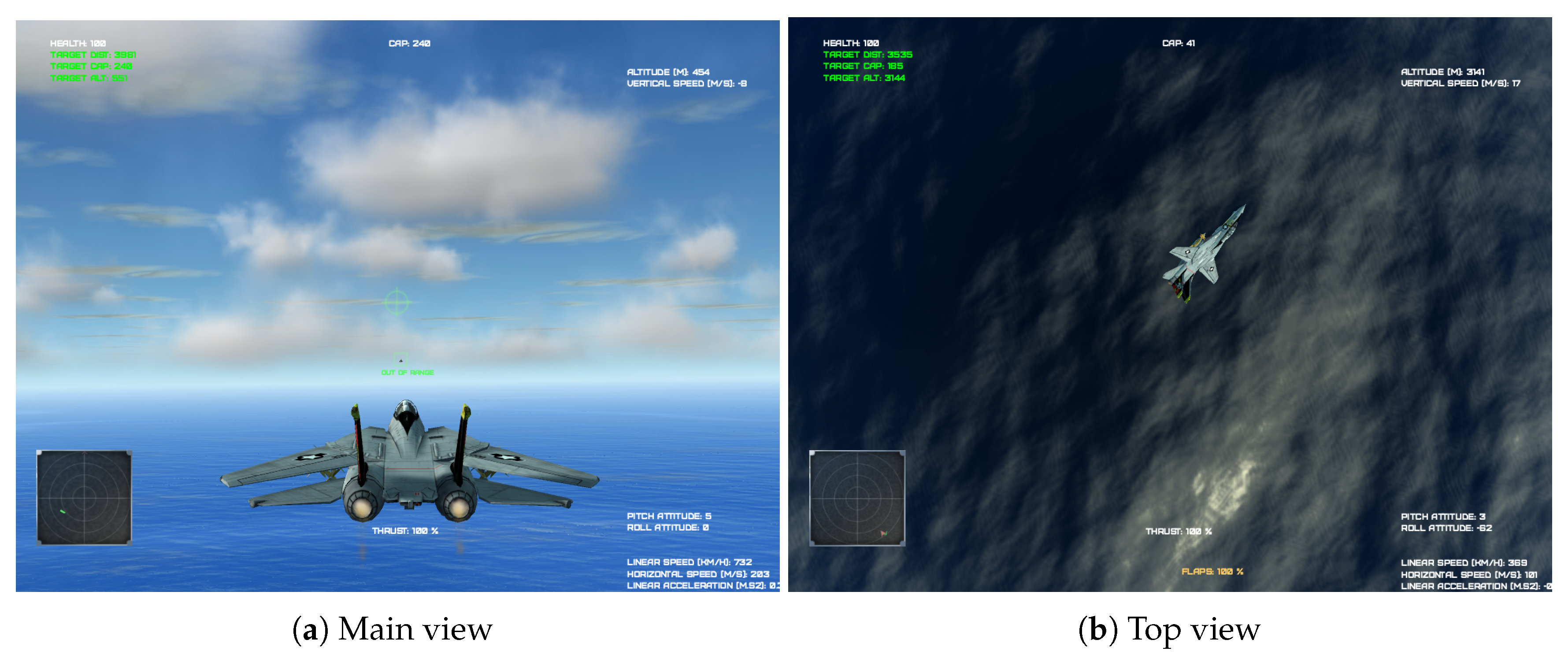
5.1.1. Aerial Combat Simulation Platform Construction

The aerial combat simulation platform was built using the HARFANG 3D framework [36], which is a software framework used for the development of modern multimedia applications and for modeling the shapes of aircraft. The HARFANG framework can manage and display complex 3D scenes, play sounds and music, and virtual reality (VR) devices. It is a new multimedia application development framework, which is highly suitable for the development of games. Nowadays, ground controllers use VR equipment to control the UAVs; hence, we adopted the HARFANG 3D framework for our proposed aerial combat simulation platform.

The platform was able to simulate the aerial combat in certain airspaces, use the dynamic equation refer in Section 3.2 to simulate the flight characteristics of aircraft, and set the performance parameters. The platform was also able to reserve the aerial combat strategy interface of the two aircraft, thereby obtaining the aircraft control signals from the external environment. The platform could also support human control, where the interface received input from a keyboard or hands-on throttle and stick system (HOTS). The graph user interface of the aerial combat simulation platform is shown in Figure 4.

The main interface of the aerial combat simulation platform is depicted in Figure 4. The interface presents a real-time combat situation of the aircraft, and the five positions on the screen display the health value, altitude and speed, radar image, attitude angle, and all the speed components.

5.1.2. Initial Setting for 1-vs-1 WVR Aerial Combat Engagement

As in Reference [37], Figure 5 shows the four different initial situation of the WVR aerial combat engagement based on the initial relative positions and orientations of the UCAVs. The initial position of the attacker concerning target in the horizontal direction is randomly chosen to be between 350 m and 1050 m in the offensive, defensive, and neutral cases. The two aircraft are at the same height initially.

5.1.3. Aircraft Performance Parameters Setting

For experimental comparison, two different aircraft performance parameters were considered in this paper. Variation of the performance capabilities focuses on the following parameters: maximum thrust and maximum angular rates, as presented in

Table 3. The aircraft performance parameters setting.

Parameter	Advantage Value	Disadvantage Value
Roll maximum rate (deg/s)	140	110
Maximum thrust (N)	100,000	80,000

. The dominant aircraft performance parameters are called the “advantage” parameters, and the non-dominant aircraft performance parameters are called the “disadvantage” parameters. The masses of both the aircraft are the same and equal to 10,000 kg each and the speed range of both the aircraft is $\left[50,250\right]$ meters per second.

5.1.4. Evaluation Metrics of Aerial Combat Strategy

The most direct method to evaluate an aerial combat strategy is to conduct an aerial combat confrontation with other aerial combat strategies and then determine the winner. We can also determine if the flight track generated by an aerial combat strategy is reasonable by observing the aircraft’s flight tracks from both sides of the combat.

To quantitatively and accurately analyze the intelligence degree of an aerial combat strategy, this study proposes four metrics: intercept time $T_I$, defensive time $T_D$, offensive time $T_O$, and winning probability $P_W$. Intercept time is measured from the aerial combat simulation’s beginning until an aircraft has a position of advantage. The position of advantage is the termination condition of the aerial combat, expressed in Equation (21). Defensive time is when a UCAV is at $\left|AA\right|>{90}^{\circ }$ during aerial combat. Offensive time is when a UCAV is at $\left|ATA\right|<{90}^{\circ }$ during aerial combat. The winning probability is the ratio of aerial combat simulations and the total number of aerial combat simulations.

5.1.5. Opponent Maueuvering Strategy

In this paper, the maneuver strategy of the target is designed using the Minimax Search Tree method (MST). The MST method simplifies and models the combat engagement between two players as a chess-type tree, a model-based method. See the schematic plot in Figure 6. The MST idea models the aircraft to following certain predefined candidate maneuvers. The candidate maneuvers include seven actions: max load factor left turn, max load factor right turn, max long acceleration, steady flight, max long deceleration, max load factor pull up, and max load factor pull over.

At each decision point, both aircraft are assumed to take actions that are prespecified as the seven elemental maneuvers. The end states of both aircraft are obtained by numerically integrating the motion equations. Given the seven potential options from each player, the terminating condition consists of 49 possibilities, represented by a seven-by-seven square matrix. Based on the terminate orientation, range, velocity, and terrain, a scoring function is defined for each index in the matrix. One player thus is to take actions that maximize the terminate score, while the other to minimize it.

The scoring function is composed of contributions consisting of an orientation score, a relative range score, and a velocity score. The contributions and the method of combining them were developed by incorporating various candidate functions into the program, performing numerous computer simulations, and studying the aircraft performance. The scoring function is defined in Equation (44).

$$Score\left(S\right)=\left[1-\frac{\left|AA\right|/\pi +\left|ATA\right|/\pi }{2}\right]e^{-\left(\left|\rho \right|-R_D\right)/\left(k\pi \right)}$$

(44)

where $R_D$ is the expected attacking range of weapons, and k is a coefficient adjusting the influence of $Score\left(S\right)$ in the total score.

5.2. Shaping Reward Experiment

5.2.1. Experiment Settings

Before using the SA-DDPG algorithm to obtain aerial combat maneuver strategy, the MaxEnt IRL algorithm is required to obtain shaping reward in order to provide the SA-DDPG algorithm. To complete the experiment, we used the aerial combat simulation platform to collect 500 different aerial combat counter trajectories manually. The initial states of these aerial combat trajectories are generated randomly, and the target uses the MST method for confrontation, and its look ahead level is set to 4.

Each component of the aerial combat features defined in Table 2 is divided into 20 parts on average, and each component of the action space is divided into five parts on average. Gradient descent method is used to solve $w*$ in Equation (42), and the learning rate is 0.01. The initial weight is set to −0.25.

5.2.2. Experiment Result and Analysis

The curve of weight w of the linear combination of features is shown in Figure 7. As can be seen from the figure, the curve showed a trend of convergence, and the weights all converge to some negative value after 6000 steps of learning. The optimal weight $w*$ are shown in

Table 4. The optimal weight $w*$ of the linear combination of aerial combat features.

Feature	$\left|\mathit{\rho }\right|$	$\left|\mathit{A}\mathit{A}\right|$	$\left|\mathit{A}\mathit{T}\mathit{A}\right|$	$|{\mathit{v}}_{\mathit{a}}-{\mathit{v}}_{\mathit{o}}|$
Optimal Weight	−0.046	−0.416	−0.515	−0.023

.

In Table 4, the weight components are all negative, which indicates that the principle of aerial combat strategy used by aerial combat experts is to reduce $\left|\rho \right|$, $\left|AA\right|$, $\left|ATA\right|$ and $|v_a-v_o|$ as much as possible to complete the aerial combat, which is intuitively reasonable.

In order to quantitatively determine the effects of the four features of the aerial combat on the total shaping reward, the color map of the shaping reward using $\left|AA\right|$ and $\left|ATA\right|$ features and the color map of the shaping reward using $\left|\rho \right|$ and $|v_a-v_o|$ features are respectively drawn in Figure 8a. In Figure 8b, the influence of $\left|AA\right|$ and $\left|ATA\right|$ on shaping reward is far greater than that of $\left|\rho \right|$ and $|v_a-v_o|$ on shaping reward. Therefore, it is more important to have the advantage of a relative angle than the advantage of relative distance and speed in aerial combat, especially in short-range aerial combat.

5.3. Performance of Training Process

5.3.1. Experiment Settings

In this section, a comparative analysis of the training methods is performed. The five training algorithms are the DDPG algorithm without reward shaping (DDPG), the DDPG algorithm with reward shaping (RS-DDPG), the SA-DDPG algorithm with reward shaping, and the learning rate $\kappa$ in Equation (33) is set to 0.1 (RS-SA-DDPG-0.1), the SA-DDPG algorithm with reward shaping and the learning rate $\kappa$ is set to 1 (RS-SA-DDPG-1), and the SA-DDPG algorithm with reward shaping and the learning rate $\kappa$ is set to 10 (RS-SA-DDPG-10) to training the aerial combat maneuver strategy.

When training the aerial combat strategies, the initial states of the two aircraft are randomly generated according to the four situations described in Section 5.1.2. At the same time, to prevent the two aircraft from falling into the “boring” Nash equilibrium of “biting the tail” during training, the performance parameters of the two aircraft to be different from one another: the attacker uses the “advantage” performance parameters, and the target uses the “disadvantage” performance parameters. The target uses the MST method for confrontation, and its look ahead level is set to 4.

The length of the actor network’s input vector is 14, and that of the output vector is 3. The length of the critic network’s input vector is 17, and that of the output vector is 1. The online actor-network, target actor-network, online critic network, and target critic network are constructed using three layers fully connected neural network, and the nodes number of the hidden layer is 64. The output layer of the actor-network and the critic network have no activation function; furthermore, the input and hidden layers are all ReLU layers. The learning rate of the network is 0.01, and the discount factor $\gamma$ is 0.9. The soft update factor of the target network is 0.01.

Additionally, the weight of the initialized neural network can be adjusted to be using the Xavier initializer. The batch size of the updating network is 1024, and the size of the experience replay memory is set to ${10}^6$. The perturbation range $ϵ$ for all normalized state components is 0.1.

5.3.2. Experiment Result and Analysis

The curve of the average reward of the aircraft shown in Figure 9. This curve is the average reward of all steps in every 500 episodes. Besides DDPG, which has only the original reward signal, the rewards of the other four algorithms all contain the shaping reward signal.

As can be seen from Figure 9, Except DDPG, the other four algorithms tend to converge. This indicated that after the introduction of the shaping reward, the algorithm’s efficiency in learning aerial combat maneuver strategy was significantly improved. By comparing the RS-DDPG algorithm with the 4 RS-SA-DDPG algorithms, it can be determined that the training convergence speed of the RS-SA-DDPG algorithms is slightly better than that of the RS-DDPG algorithm, and the final convergence result of RS-SA-DDPG algorithms is better than the RS-DDPG algorithm. By comparing the convergence curves of three RS-SA-DDPG algorithms with different $\kappa$ parameters, the convergence speed will be slightly slower with the increase of $\kappa$, and it can converge to a better result, to obtain a better aerial combat maneuver strategy.

5.4. Testing Aerial Combat Maneuver Strategy

5.4.1. Experiment Settings

In this section, the intelligence degree of aerial combat maneuver strategy obtained using the RS-SA-DDPG-1 algorithm is evaluated against the target using the uniform linear motion maneuver strategy and four look-ahead MST maneuver strategy. The performance parameters of aircraft on both sides are kept at “Advantage” to ensure that the performance of the two aircraft is the same. The perturbation range $ϵ$ is 0.1. Meanwhile, the initial situation of the attacker is set to “Defensive” when the attacker conducts aerial combat with the target with the uniform linear motion maneuver strategy; the initial situation of the attacker is set to “Opposite” when the attacker conducts aerial combat with the target with the MST maneuver strategy.

5.4.2. Experiment Result and Analysis

The results of the simulation scenario against the uniform linear motion maneuver strategy are presented in Figure 10. The trajectories are depicted at intervals of 1 second. The downward-pointing triangle points at the trajectory represent the initial position. The cross points at the trajectory represent the end position of the aerial combat and, the circular points are marked every 10 s. To gain the situational advantage in aerial combat, the attacker performs a somersault maneuver to allow the target to overshoot it for about 30 s quickly. Then, the attacker speeds up to catch up with the opponent and, finally, slows down to prevent overshoot and steadily tracks the target. As a result, the target was successfully destroyed in 50 s by gunshot. It can also be seen from Figure 10 that the overall features of the attacker relative to the target increases from the initial positive value to zero, and there are some oscillations in the middle, but in the end, it can be stably maintained at zero, i.e., in an advantageous situation.

The results of the simulation scenario against the four look-ahead MST maneuver strategy are presented in Figure 11. The attacker first accelerates to approach the target and overshoot quickly for about 20 s, and the target takes an advantageous situation. Then at 30 s, the attacker makes the left turn to bring the aircraft into the opposite situation. After 50 s, the attacker takes an advantageous position. Although the target adopted a series of maneuvers of acceleration or turning to try to get rid of it, the agent aircraft is still in an advantageous situation and gradually stabilized tracking.

From the above two simulation results, it can be concluded that the aerial combat maneuver strategy using the RS-SA-DDPG-1 algorithm is effective. Besides, 1000 times Monte-Carlo simulations with the randomly initial situations were performed to ensure the universal validity of the performance in air combats between the strategies of the RS-SA-DDPG-1 algorithm and the four look-ahead MST method. The results are presented in Figure 12. As can be seen from Figure 12, regardless of the initial aerial combat situations, RS-SA-DDPG-1 strategy wins the air combats with a high probability, and the total probability of winning reaches 63.01%, and the average intercept time is 60.09 s.

5.5. Robustness Evaluation of the Aerial Combat Maneuver Strategy

5.5.1. Experiment Settings

In this section, in order to test the robustness of the aerial combat strategy, two experiments are designed. First, we modified the perturbation range $ϵ$ to evaluate the impact on the effectiveness of aerial combat strategies obtained by RS-SA-DDPG-1 and RS-DDPG algorithms. The perturbation range $ϵ$ is set to $\{0,0.1,0.2,0.3,0.4\}$. For each perturbation range, we will conduct 1000 aerial combat simulations, and the initial aerial combat states are randomly generated to record the result of each aerial combat. Then, we modified the look ahead level of the aerial combat strategy of the target using the MST method to evaluate the impact on the effectiveness of aerial combat strategies obtained by RS-SA-DDPG-1 and RS-DDPG algorithms. The look-ahead level is set from 1 to 6. For each look ahead level, we will conduct 1000 aerial combat simulations, and the initial aerial combat states are randomly generated to record the result of each aerial combat.

5.5.2. Experiment Result and Analysis

The result of the experiment is shown in Figure 13. Firstly, the robustness of the airial combat strategy on the perturbation range of observation error is analyzed. In Figure 13a, when the perturbation range $ϵ$ is 0, the winning rate of aerial combat strategies obtained by RS-SA-DDPG-1 and RS-DDPG algorithms are relatively high, about 0.8. This shows that the introduction of the regularization of robustness will not affect the performance of the airial combat strategy network. With the increase of the perturbation range $ϵ$, the winning rate of aerial combat strategies obtained by RS-SA-DDPG-1 algorithm remained relatively stable, and the winning rate of aerial combat strategies obtained by RS-DDPG algorithm gradually declined to about 40%. This shows that the robustness of the policy network with regularization is better than that without regularization. Then, the robustness of the airial combat strategy on the target intelligence level is analyzed. In Figure 13b, with the increase of the look ahead level of target, the winning rate of aerial combat strategies obtained by RS-SA-DDPG-1 and RS-DDPG algorithm gradually decrease simultaneously, but the rate of decline of RS-SA-DDPG-1 is less than the rate of decline of RS-DDPG. Through these two experiments, it can be found that the robustness of the aerial combat strategies obtained by the RS-SA-DDPG-1 algorithm is better than that of the aerial combat strategies obtained by the RS-DDPG algorithm no matter changing the perturbation range $ϵ$ or the intelligence degree of the target.

6. Conclusions

In order to generate intelligent and robust aerial combat maneuver strategy, an algorithm for generating the aircraft’s autonomous maneuver strategy based on the SA-DDPG algorithm and inverse reinforcement learning algorithm is proposed in this paper. In order to model the measurement errors of the sensors of aircraft in aerial combat, the process of aerial combat is modeled as SA-MDP. As can be seen from the experimental results above, the shaping reward obtained through the inverse reinforcement learning algorithm can effectively improve the speed of the aerial combat strategy learning. Meanwhile, through the comparison of aerial combat simulation results of the aerial combat strategies obtained by DDPG, SA-DDPG algorithm, it can be found that the aerial combat strategies obtained by the SA-DDPG algorithm have strong robustness. In this paper, only the decision of aircraft maneuver is studied, but the control strategy of weapon and sensor is not discussed, which needs study in the future.

References

1. Skjervold, E. Autonomous, Cooperative UAV Operations using COTS Consumer Drones and Custom Ground Control Station. In Proceedings of the MILCOM 2018—2018 IEEE Military Communications Conference (MILCOM), Los Angeles, CA, USA, 29–31 October 2018; pp. 1–6. [Google Scholar]
2. Gupta, S.G.; Ghonge, D.; Jawandhiya, P.M. Review of unmanned aircraft system (UAS). Int. J. Adv. Res. Comput. Eng. Technol. (IJARCET) Vol. 2013, 2, 1646–1658. [Google Scholar] [CrossRef]
3. Hebert, A.J. Fighter generations. Air Force Mag. 2008, 91, 1. [Google Scholar]
4. Ardema, M.; Rajan, N. An Approach to Three-dimensional Aircraft Pursuit–evasion. In Pursuit-Evasion Differential Games; Elsevier: Amsterdam, The Netherlands, 1987; pp. 97–110. [Google Scholar]
5. Park, H.; Lee, B.Y.; Tahk, M.J.; Yoo, D.W. Differential game based air combat maneuver generation using scoring function matrix. Int. J. Aeronaut. Space Sci. 2016, 17, 204–213. [Google Scholar] [CrossRef] [Green Version]
6. Jarmark, B.; Hillberg, C. Pursuit-evasion between two realistic aircraft. J. Guid. Control Dyn. 1984, 7, 690–694. [Google Scholar] [CrossRef]
7. Greenwood, N. A differential game in three dimensions: The aerial dogfight scenario. Dyn. Control 1992, 2, 161–200. [Google Scholar] [CrossRef]
8. McGrew, J.S.; How, J.P.; Williams, B.; Roy, N. Air-combat strategy using approximate dynamic programming. J. Guid. Control Dyn. 2010, 33, 1641–1654. [Google Scholar] [CrossRef] [Green Version]
9. Shin, H.; Lee, J.; Kim, H.; Shim, D.H. An autonomous aerial combat framework for two-on-two engagements based on basic fighter maneuvers. Aerosp. Sci. Technol. 2018, 72, 305–315. [Google Scholar] [CrossRef]
10. Burgin, G.H.; Owens, A. An Adaptive Maneuvering Logic Computer Program for the Simulation of One-to-One Air-to-Air Combat. Volume 2: Program Description; Technical Report; NASA: Washington, DC, USA, 1975. [Google Scholar]
11. Chappell, A.R. Knowledge-based Reasoning in the Paladin Tactical Decision Generation System. In Proceedings of the IEEE/AIAA 11th Digital Avionics Systems Conference, Seattle, WA, USA, 5–8 October 1992; pp. 155–160. [Google Scholar]
12. Chappell, A.; Mcmanus, J.; Goodrich, K. Trial Maneuver Generation and Selection in the PALADIN Tactical Decision Generation System. In Proceedings of the Astrodynamics Conference, Hilton Head, SC, USA, 10–12 August 1992; p. 4541. [Google Scholar]
13. Virtanen, K.; Raivio, T.; Hämäläinen, R.P. An Influence Diagram Approach to One-on-one Air Combat. In Proceedings of the 10th International Symposium on Differential Games and Applications, St. Petersburg, Russia, 8–11 July 2002; Volume 2, pp. 859–864. [Google Scholar]
14. Virtanen, K.; Karelahti, J.; Raivio, T. Modeling air combat by a moving horizon influence diagram game. J. Guid. Control Dyn. 2006, 29, 1080–1091. [Google Scholar] [CrossRef] [Green Version]
15. McMahon, D.C. A Neural Network Trained to Select Aircraft Maneuvers during Air Combat: A Comparison of Network and Rule based Performance. In Proceedings of the 1990 IJCNN International Joint Conference on Neural Networks, San Diego, CA, USA, 17–21 June 1990; pp. 107–112. [Google Scholar]
16. Teng, T.H.; Tan, A.H.; Tan, Y.S.; Yeo, A. Self-organizing Neural Networks for Learning Air Combat Maneuvers. In Proceedings of the 2012 International Joint Conference on Neural Networks (IJCNN), Brisbane, Australia, 10–15 June 2012; pp. 1–8. [Google Scholar]
17. Bo, L.; Zheng, Q.; Liping, S.; Youbing, G.; Rui, W. Air Combat Decision Making for Coordinated Multiple Target Attack Using Collective Intelligence. Acta Aeronaut. Astronaut. Sin. 2009, 9, E926. [Google Scholar]
18. Yang, Z.; Zhou, D.; Piao, H.; Zhang, K.; Kong, W.; Pan, Q. Evasive Maneuver Strategy for UCAV in Beyond-Visual-Range Air Combat Based on Hierarchical Multi-Objective Evolutionary Algorithm. IEEE Access 2020, 8, 46605–46623. [Google Scholar] [CrossRef]
19. Yang, Q.; Zhu, Y.; Zhang, J.; Qiao, S.; Liu, J. UAV Air Combat Autonomous Maneuver Decision Based on DDPG Algorithm. In Proceedings of the 2019 IEEE 15th International Conference on Control and Automation (ICCA), Edinburgh, UK, 16–19 July 2019; pp. 37–42. [Google Scholar]
20. Zuo, Y.; Deng, K.; Yang, Y.; Huang, T. Flight Attitude Simulator Control System Design based on Model-free Reinforcement Learning Method. In Proceedings of the 2019 IEEE 3rd Advanced Information Management, Communicates, Electronic and Automation Control Conference (IMCEC), Chongqing, China, 11–13 October 2019; pp. 355–361. [Google Scholar]
21. Radac, M.B.; Lala, T. Learning Output Reference Model Tracking for Higher-Order Nonlinear Systems with Unknown Dynamics. Algorithms 2019, 12, 121. [Google Scholar] [CrossRef] [Green Version]
22. Qi, H.; Hu, Z.; Huang, H.; Wen, X.; Lu, Z. Energy Efficient 3-D UAV Control for Persistent Communication Service and Fairness: A Deep Reinforcement Learning Approach. IEEE Access 2020, 36, 53172–53184. [Google Scholar] [CrossRef]
23. Song, H.; Liu, C.C.; Lawarrée, J.; Dahlgren, R.W. Optimal electricity supply bidding by Markov decision process. IEEE Trans. Power Syst. 2000, 15, 618–624. [Google Scholar] [CrossRef]
24. Bernstein, D.S.; Givan, R.; Immerman, N.; Zilberstein, S. The complexity of decentralized control of Markov decision processes. Math. Oper. Res. 2002, 27, 819–840. [Google Scholar] [CrossRef]
25. Bellman, R. A Markovian decision process. J. Math. Mech. 1957, 6, 679–684. [Google Scholar] [CrossRef]
26. Bellman, R. The Theory of Dynamic Programming. Bull. Amer. Math. Soc. 1954, 60, 503–515. [Google Scholar] [CrossRef] [Green Version]
27. Zhang, H.; Chen, H.; Xiao, C.; Li, B.; Boning, D.; Hsieh, C.J. Robust Deep Reinforcement Learning against Adversarial Perturbations on Observations. arXiv 2020, arXiv:2003.08938. [Google Scholar]
28. Lillicrap, T.P.; Hunt, J.J.; Pritzel, A.; Heess, N.; Erez, T.; Tassa, Y.; Silver, D.; Wierstra, D. Continuous control with deep reinforcement learning. arXiv 2015, arXiv:1509.02971. [Google Scholar]
29. Mnih, V.; Kavukcuoglu, K.; Silver, D.; Graves, A.; Antonoglou, I.; Wierstra, D.; Riedmiller, M. Playing atari with deep reinforcement learning. arXiv 2013, arXiv:1312.5602. [Google Scholar]
30. Schaul, T.; Quan, J.; Antonoglou, I.; Silver, D. Prioritized experience replay. arXiv 2015, arXiv:1511.05952. [Google Scholar]
31. Gowal, S.; Dvijotham, K.; Stanforth, R.; Bunel, R.; Qin, C.; Uesato, J.; Arandjelovic, R.; Mann, T.; Kohli, P. On the effectiveness of interval bound propagation for training verifiably robust models. arXiv 2018, arXiv:1810.12715. [Google Scholar]
32. Laud, A.D. Theory and Application of Reward Shaping in Reinforcement Learning. Technical Report. 2004. Available online: https://www.ideals.illinois.edu/handle/2142/10797 (accessed on 8 July 2020).
33. Ng, A.Y.; Russell, S.J. Algorithms for Inverse Reinforcement Learning. In Proceedings of the International Conference on Machine Learning (ICML), Stanford, CA, USA, 29 June–2 July 2000; Volume 1, p. 2. [Google Scholar]
34. Ziebart, B.D.; Maas, A.L.; Bagnell, J.A.; Dey, A.K. Maximum Entropy Inverse Reinforcement Learning. In Proceedings of the Association for the Advancement of Artificial Intelligence (AAAI), Chicago, IL, USA, 13–17 July 2008; Volume 8, pp. 1433–1438. [Google Scholar]
35. Jaynes, E.T. On the rationale of maximum-entropy methods. Proc. IEEE 1982, 70, 939–952. [Google Scholar] [CrossRef]
36. Nichols, R.; Ryan, J.; Mumm, H.; Lonstein, W.; Carter, C.; Hood, J. Africa–World’s First Busiest Drone Operational Proving Ground. In Unmanned Aircraft Systems in the Cyber Domain; New Prairie Press: Manhattan, KS, USA, 2019. [Google Scholar]
37. Ramírez López, N.; Żbikowski, R. Effectiveness of autonomous decision making for unmanned combat aerial vehicles in dogfight engagements. J. Guid. Control Dyn. 2018, 41, 1021–1024. [Google Scholar] [CrossRef]
Figure 1. The diagrammatic sketchs of MDP and SA-MDP.
Electronics 09 01121 g001
Figure 2. The geometric situation of the aerial combat.
Electronics 09 01121 g002
Figure 3. Aerial combat maueuvering strategy generation algorithm using SA-DDPG.
Electronics 09 01121 g003
Figure 4. The graph user interface of the aerial combat simulation platform.
Electronics 09 01121 g004
Figure 5. The four different initial situation of the WVR aerial combat engagement.
Electronics 09 01121 g005
Figure 6. A schematic plot of the MST. Agent and Opponent indicate two aircraft.
Electronics 09 01121 g006
Figure 7. The convergence curve of weight w of the linear combination of aerial combat features.
Electronics 09 01121 g007
Figure 8. The effects of the 4 features of the aerial combat on the shaping reward.
Electronics 09 01121 g008
Figure 9. The convergence curve of weight w of the linear combination of aerial combat features.
Electronics 09 01121 g009
Figure 10. The simulation results of the aerial combat maneuver strategy using the RS-SA-DDPG-1algorithm against the uniform linear motion maneuver strategy.
Electronics 09 01121 g010
Figure 11. The simulation results of the aerial combat maneuver strategy using the RS-SA-DDPG-1 algorithm against the uniform linear motion maneuver strategy.
Electronics 09 01121 g011
Figure 12. The results of the 1000 times aerial combat simulations.
Electronics 09 01121 g012
Figure 13. The results for robustness evaluation of the aerial combat maneuver strategy.
Electronics 09 01121 g013