Combining Machine Learning Analysis and Incentive-Based Genetic Algorithms to Optimise Energy District Renewable Self-Consumption in Demand-Response Programs

Abstract

The recent rise of renewable energy sources connected to the distribution networks and the high peak consumptions requested by electric vehicle-charging bring new challenges for network operators. To operate smart electricity grids, cooperation between grid-owned and third-party assets becomes crucial. In this paper, we propose a methodology that combines machine learning with multi-objective optimization to accurately plan the exploitation of the energy district’s flexibility with the objective of reducing peak consumption and avoiding reverse power flow. Using historical data, acquired by the smart meters deployed on the pilot district, the district’s power profile can be predicted daily and analyzed to identify potentially critical issues on the network. District’s resources, such as electric vehicles, charging stations, photovoltaic panels, buildings energy management systems, and energy storage systems, have been modeled by taking into account their operational constraints and the multi-objective optimization has been adopted to identify the usage pattern that better suits the distribution operator’s (DSO) needs. The district is subject to incentives and penalties based on its ability to respond to the DSO request. Analysis of the results shows that this methodology can lead to a substantial reduction of both the reverse power flow and peak consumption.

1. Introduction

Nowadays in Europe more than 90% of the renewable distributed generators are connected to the distribution grid [1]. In recent years, in fact, a massive number of renewable energy sources (RES) has been installed thanks to the advantageous fiscal policies and to the various incentives that have been put in place at the national level. The explosion of RES connections has led to new challenges for the stakeholders and particularly for the Distribution System Operator (DSO) that is tasked with ensuring and enhancing power quality for consumers and producers. These challenges have made a pressing need for smartening the electricity grids, demand response (DR) and demand-side management strategies are adopted to increase system efficiency [2,3], accurate forecasting algorithms are more crucial than ever [4,5].

The need to optimize the operation of integrated energy systems is a subject of particular interest at present. Optimal scheduling of combined heat and power operations, considering thermal inertia of buildings can improve renewable energy consumption, as in [6]. Ghasemi et al. [7] proposed an optimization framework to balance non-dispatchable renewable power generation and demand using pumped-storage units. In the presence of high renewable energy integration, load shifting and power-controlled heat supply can contribute to reducing energy supply cost and $C{O}_2$ emission [8]. The potential for demand response strategies and battery storage systems (BSS) has been compared, showing that both BSS and DR could enhance the self-consumption of photovoltaics (PV) generation in residential contexts [9]. At the same time, electric vehicles are emerging as resources able to provide flexibility services to DSOs [10,11,12].

Applying Machine Learning (ML)-based methods has resulted in a major improvement in different fields. A recent study [13] successfully applied, in the industry field, a Random Forest (RF)-based ML technique to minimize the makespan of an Unrelated Parallel Machines Scheduling Problem (UPMSP) considering setup time uncertainties in a machine-dependent and job sequence-dependent scheduling environment. In cloud computing areas, the Artificial Neural Network (ANN) method was used to predict virtualized resource-allocation in order to solve a multi-objective task scheduling model, minimizing energy consumption and makespan [14]. Machine learning is a very promising approach also for network traffic classification. Nascimento et al. [15] proposed a hybrid model which combines a classifier based on computational intelligence, the Extreme Learning Machine (ELM), along with Feature Selection (FS) and Multi-objective genetic algorithms to classify computer network traffic without making use of the payload or port information.

Trying to achieve similar results in our context, in this paper we present a novel ML-evolutionary model to optimize renewables self-consumption on a district level. A linear regression model is optimized through a multiple objective optimization algorithm combined with correction factors modeling the weather conditions. The model identifies the potential configuration of different flexibility resources in a district in order to accomplish the DSO power profile requests. The DSO power profile request is to be intended as a resolution of congestion issues or reduction of production/consumption peaks at certain hours of the day, depending on the specific needs of the grid during the request. An incentive/penalty mechanism is also applied for the provision of service. The district can follow the DSO power profile more or less carefully; incentives are proportional to the accuracy achieved by district prosumers (i.e., energy consumers with production capabilities). Vice versa, the incentives decrease until they become negative, representing penalties to be paid to the DSO. On the other hand, the more the district moves away from its forecast to follow the DSO profile, the more it is compensated for its effort.

The paper is organized as follows. In Section 2, the overall methodology is presented. Then, Section 3 analyzes the results from our pilot trial, from which we deduce conclusions presented in Section 4.

2. Methods

The process we are going to propose is triggered by the DSO sending its service request to the district aggregator. The request is based on the prediction of energy consumption and production of the district. There exist different techniques to forecast energy production/consumption [16]. ML techniques give better performance in this context and are preferred in many studies [17,18,19]. When the ML models are trained with enough amount of data, they can be used to predict targets for unseen samples, though the relation between the features and the targets is not defined. This procedure is also known as supervised learning in the ML field. Two types of supervised ML algorithms exist: regression and classification. The former predicts continuous value outputs while the latter predicts discrete outputs. In this work, we use a linear regression model to predict the production/consumption output power profiles in a district. The algorithm takes as input a sufficiently large dataset and some critical variables (or decision variables) and returns a linear model based on the critical variables. The model coefficients are calculated on the historical data to present in the dataset.

In order to find the best combination of decision variables in the regression model, i.e., the combination that minimizes the Normalized Root Mean Squared Deviation (NRMSD) in M different test samples, it is exploited an optimization algorithm, the Non-dominated Sorting Genetic Algorithm II (NSGA-II) [20]. This algorithm is based on Pareto-dominance and Pareto-optimality and many papers in the literature have proved its efficiency, also in the field of power distribution operation and planning [21,22,23,24]. In fact, the same algorithm is used from the district to find the optimized power profile in response to the DSO request. The optimized profile is determined by minimizing/maximizing a combination of three objective functions that address the management criteria of the district: one function is the total price of energy (this function is minimized), the other two functions, that are maximized, are the sum of all incentives paid by the DSO to the district flexibility providers and the number of time-slots where the profile is within the tolerance range, respectively.

2.1. Case Study

As a case study, the dataset is related to a district located at the premises of DSO of the city of Terni, in Italy, namely Terni Distribuzione Elettrica (TDE) which is a production unit of ASM Terni SpA. The district is composed of: two PV arrays (180 kWp and 60 kWp), connected to the LV network; a block of three office buildings which is considered as a load and does not have any controllable system; a storage system able to provide active power up to 72 kW having a total capacity of 66 kWh; three smart charging stations (2 AC current, rated power 22 kW, 1 DC current, 52 kW) and six electric vehicles, used by employees (see Figure 1). In this context, the aggregated forecast of the district is calculated as the sum of photovoltaic forecast production and building forecast consumption. The convention adopted here considers the positive power flows as power consumption and the negative ones as power generation. The dataset considered for our case study includes a time window from 13 June 2018 at 00:00 to 11 June 2019 at 23:50.

2.2. Architecture

The software architecture developed in our prototype implementation is shown in Figure 2, together with the external services used and the hardware smart-meters, it exploits FIWARE [25] generic enabler for data brokering.

To perform our multiple linear regression, we are using, as input features, two data sources: the first one is the set of historical data acquired in our pilot site, while the second one is a set of historical weather data for the same time window. To train the algorithm, the two data sources are combined together, and the final subset of input features is selected using an implementation of the NSGA-II genetic algorithm to determine the best model. The forecasts calculated using this model, together with the load profile requested by the DSO, and the function describing the evolution in time of the energy price are finally used to calculate the optimized prosumer’s load profile for each request, again, using an implementation of the NSGA-II algorithm.

Smart Meters

Each smart meter continuously transmits its readings on its own dedicated Message Queue Telemetry Transport (MQTT) topic. To manage the Internet of Things (IoT) context information, the platform implements a solution based on FIWARE, a framework of open source components aimed at the development of smart applications, in particular, it integrates three FIWARE generic enablers: Orion Context Broker, IoT Agent for JSON and Short Time Historic. To manage the lifecycle and the availability of context information we use the Orion Context Broker, an NGSIv2 server implementation. To manage our IoT devices using their own native protocol, we’re using an IoT Agent for JSON to convert messages from JSON to NGSI and vice-versa. Finally, we use the Short Time Historic (STH) component to store and retrieve historical context information. STH stores raw and aggregated data using a MongoDB database.

2.3. Forecast

In this chapter, the optimal forecast for the different district assets is determined as the first step. Further, those forecasts are used for the district optimization in terms of district flexibilities combination to match the DSO power profile request. The process followed in this research to obtain a forecast starting from historical data can be summarized by the steps illustrated in Figure 3. The raw data, transmitted by smart meters, were stored in a database. This dataset, before being used for algorithm training, was verified, filtered, and aggregated to the required granularity, ten-minute timeslots in our case. The dataset was then partitioned, so that 80% was used for training and the remaining 20% for the validation of results. The training was then repeated using various subsets of critical variables during the optimization process and, at the end of this process, the subset that generated the lowest error on a different set of randomly selected test partitions is chosen. Finally, the resulting model is ready to generate new forecasts.

The weather has a significant impact on forecasting power profiles. A number of studies have investigated the effect of weather variables on building energy consumption. Amber, et al. [26] investigated the effect of four weather variables, i.e., the surrounding temperature, global irradiance, humidity and wind velocity on the electricity usage of different buildings. Among the four variables, the surrounding temperature found to be the critical parameter that drives the building energy consumption. Braun et al. [27] also found that among outdoor temperature and humidity the former plays a dominant role in building energy consumption. On the other hand, Al-Garni et al. [28], with variable occupant populations, found the relative humidity and global irradiance as the critical variables as the main driving force for the building energy consumption. Other studies show how the power output from a PV array is extremely dependant on environmental variables such as irradiance, temperature, wind speed, humidity, air pressure, and sky conditions [29,30]. Previous works have shown that the lack of accurate information about these variables can affect the prediction error significantly [31]. To assess the effects of weather variables in the forecasting model presented in this paper, weather data are retrieved by third party service available on-line, World Weather Online [32]. The observed weather variables provided by the service are acquired by hourly resolution during the studying time via API requests and include outdoor temperature, wind speed, humidity, visibility, air pressure, cloud cover, dew point, UV index. The selected variables and the online service were chosen to evaluate the performances using a commonly available data source, instead of other influencing factors, such as solar radiation, that even if they could provide a more precise prediction could not be accessible for typical small scale prosumers. A Multiple Linear Regression algorithm was used to predict the district power profile for a specific date. The implementation of the algorithm is based on the Python Scikit-Learn library, which is one of the most popular machine learning libraries for Python [33]. The forecast model can be defined as:

$$\begin{gathered} f_t=b_0{v}_0+b_1{v}_1+b_2{v}_2+b_3{v}_3+b_4{v}_4+b_5{v}_5 \\ +b_6{v}_6+b_7{v}_7+b_8{v}_8+b_9{v}_9+b_{10}{v}_{10}+b_{11}{v}_{11}+b_{12}{v}_{13}+b_{14}{v}_{14}, \end{gathered}$$

where $f_t$ is our forecast at time t, while $v_i$$\forall i\in \{0,\dots ,5\}$ are called critical variables and represent the historical dates (each critical variable is a triplet value of Day, Hour, Minutes in the past) used for the calculation of the forecast. $v_i$$\forall i\in \{6,\dots ,14\}$ represent weather variables. Finally $b_i$$\forall i\in \{0,\dots ,14\}$ are the coefficients applied, at the end of the algorithm execution, to the independent variables. In order to understand which is the best combination of critical variables to choose for the calculation of the forecast, many tests should be performed and errors should be analyzed. In Section 2.4 we present a novel approach based on an optimization algorithm, which enables us to find the optimized combination of critical variables.

2.4. Optimization of the Forecast

The Non-dominated Sorting Genetic Algorithm II (NSGA-II) [20] is the most frequently used evolutionary multi-objective optimization algorithm in the literature. In a previous work, [11] its reliability and performance has already been demonstrated. A later version of the algorithm has been proposed, i.e., NSGA-III [34], however it is more suitable for many objective problems, while NSGA-II has proven to be performing well in the case of bi-objective models [35]. Further comparison between NSGA-II and other evolutionary algorithms has been reported in the literature. In this study [36], authors compared four multi-objective evolutionary algorithms for Water Distribution Networks (WDN) design optimization entitled NSGA-II, Multi-Objective Genetic Algorithm (MOGA), Niched Pareto Genetic Algorithm (NPGA) and Pareto Archived Evolution Strategy (PAES). They found that the NSGA-II was the best of the tested algorithms.

The objective of the NSGA-II algorithm is to improve the adaptive fit of a population of candidate solutions to a Pareto front constrained by a set of objective functions. The algorithm uses an evolutionary process with surrogates for evolutionary operators including selection, genetic crossover and genetic mutation. The population is sorted into a hierarchy of sub-populations based on the ordering of Pareto dominance. Similarity between members of each sub-group was evaluated on the Pareto front, and the resulting groups and similarity measures were used to promote a diverse front of non-dominated solutions. It is important to strike a balance between the forecast accuracy and the computational cost: the critical variables selection was subjected to diminishing returns so, after a certain number, adding more variables to the pool does not improve the results significantly while the computational cost increases. Considering V the number of critical variables, their optimal selection is the one that minimizes the M objective functions. Each set of V elements from the whole space of possible critical variables is considered an individual. The genetic algorithm proceeds to generate N individuals forming the initial population, and calculating the M objective functions against each individual. A child population was then created combining the crossover and mutation genetic operators with $\mu$ and $\widehat{\mu }$ probabilities. The two populations are then joined together and sorted based on the results of the objective functions. Finally, the best N individuals are selected to form a new population. This process is repeated G times, refining the population after each iteration. We decided to apply this process to find a subset of historical production/consumption data that would provide the best results in terms of forecasting and then combine the results with weather data to obtain an accurate forecast of energy production or consumption.

2.5. Power Profile Optimization

Once determined the optimal forecast for each asset, those are combined with the available flexibilities in order to achieve the DSO power profile request for the district as a whole. The optimized profile that the district will follow is calculated trying to maximize the incentives to be received for the provided flexibility, maximize the number of timestamps in which the power profile is following the DSO’s request, and minimizing the overall cost considering the energy price variation during the day. Each condition has been formalized as an objective function. Incentives, or penalties, were calculated following the model already proposed in [37] using the formula described in Equation (1), where for each 10 minutes timeslot: t, $r_t$ is the requested power profile, $f_t$ is the forecasted power profile, and $d_t$ represents the optimized power profile. M and R are the penalty multiplier and the tolerance range for the request (with M = 0.5 and R = 8 kW in our case).

$$I(t,R,M)=\left\{\begin{array}{cc}\frac{1}{R}(R-|r_t-d_t\left|\right)e^{-\frac{|r_t-d_t|}{|r_t-f_t|}}\hfill & \mathrm{when}|r_t-d_t|\le R\mathrm{and}|r_t-f_t|>0\hfill \\ \frac{1}{R}(R-|r_t-d_t\left|\right)e^{-|r_t-d_t|}\hfill & \mathrm{when}|r_t-d_t|\le R\mathrm{and}|r_t-f_t|=0\hfill \\ \frac{M}{R}(R-|r_t-d_t\left|\right)e^{-\frac{|r_t-f_t|}{|r_t-d_t|}}\hfill & \mathrm{when}|r_t-d_t|>R\hfill \end{array}\right.$$

(1)

The same tolerance range was used to determine the number of timeslots in which the optimized profile follows the DSO’s request.

To generate the optimized profile, the NSGA-II algorithm was used to try allocating the resources which provide flexibility available on the pilot site. In addition to the already mentioned PV panels and buildings, the pilot site features also a district energy storage system and a set of electric vehicles charging stations and e-cars (three charging stations and a fleet of six electric vehicles).The electric vehicles provide flexibility in terms of charge shift, while the district battery provides flexibility as charging power modulation. The district energy storage system exploits a second-life battery solution, developed as part of the ELSA project, composed by a set of six second-life batteries for Renault Kangoo, with a total capacity of 66 kWh, a maximum charging power of 72 kW, and a maximum discharge power of 72 kW. The algorithm takes as initial states of charge for any given day the final states of charge of the previous day. In this case, we simulated the initial states of charge trying to represent a life-like configuration loading each resource between 30% and 50% of its maximum capacity. The EVs fleet was composed of two Nissan Leaf (capacity 24 kWh, peak charging power: 7 kW), two first-generation Renault Zoe (capacity 22 kWh, peak charging power: 22 kW), and two second-generation Renault Zoe (capacity 41 kWh, peak charging power: 22 kW). Electric vehicles can be recharged at three charging points: two with a peak power output of 22 kW and the third one with a peak power output of 52 kW. Each charging station had two independent sockets. Modeling the pilot, the resource natural limitations and additional constraints have been taken into account. The natural limitations are easily deducible: vehicles and the energy storage system cannot be charged to more than their maximum capacity, the energy storage system cannot be discharged below 0 kWh, and only one vehicle at time can be charged using the same charging socket. The only constraint that was imposed was that the same vehicle cannot be recharged another time later on the same day and or using another charging station after that is connected to a charging station.

The resource models (as decision variables and constraints), together with the three objective functions are used as inputs for the NSGA-II algorithm already described in Section 2.4. The optimizer returns, for each timeslot, the power at which to charge or discharge the battery (to indicate a discharge negative values are used as charging power) and the list of which vehicles to recharge in which charging station. The recommended profile was obtained by adding the information received from the optimizer to the power profile forecast.

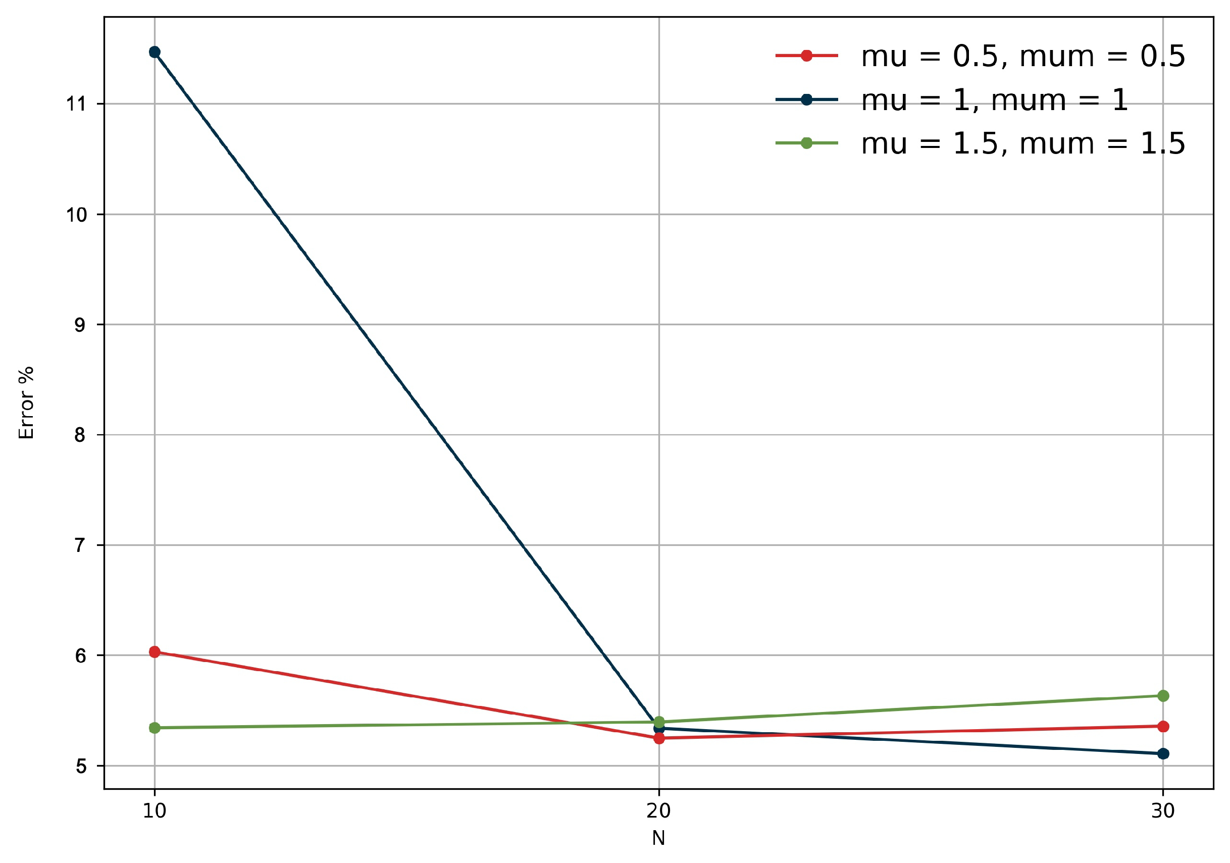
2.6. Calibration of NSGA-II Parameters

To calibrate the parameters of the NSGA-II optimizer, a two-step process was followed, trying to find the best balance between system performance and result quality. In the first step, the population size and the crossover and mutation rates were selected after comparing different configurations over a relatively small number of iterations to obtain the lowest NRMSD % and the highest Reverse Power Flow (RPF) reduction %. In the second step, the selected values were tested over an increasing number of iterations, until an acceptable threshold was reached.

From Figure 4, we can see that the lowest error % was obtained with a population size of 30 individuals, a crossover rate of 1, and a mutation rate of 1. Figure 5 shows that with the above parameters, the error % resulted below 4.85 after 1000 iterations.

The tests for the optimization of the power profile demonstrated that the best combination in reducing the RPF % is obtained with a population of 20 individuals, 1 as mutation rate, and 1 as crossover rate (Figure 6). The parameters above resulted in a reduction of the RPF over 80% after 1200 iterations (Figure 7).

3. Results and Discussion

The following subsections report the results of the optimization process. Although NSGA-II is a heuristic search method, able to converge to solutions containing certain randomness, the process was designed to mitigate randomness effect: in the optimization of the forecast, we validate for each iteration the resulting model against different validation sets. In the optimization of the power profile, the objective functions are designed to follow the DSO request and to consider the limits of the available resources, avoiding unpredictable results.

To assess the system scalability, it is worth noticing that the computational cost of the methodology proposed depends mostly on the evolutionary algorithm, NSGA-II. More specifically, a Fast Elitist Non-Dominated Sorting Genetic Algorithm for Multi-Objective Optimization [20] was used. Its computational cost depends on the cost of the sorting procedure $O\left(M{N}^2\right)$, where M is the number of objective functions and N is the population size. Since the overall cost of the sorting procedure is not affected by the number of the district’s resources, the proposed solution could be scaled to larger platforms.

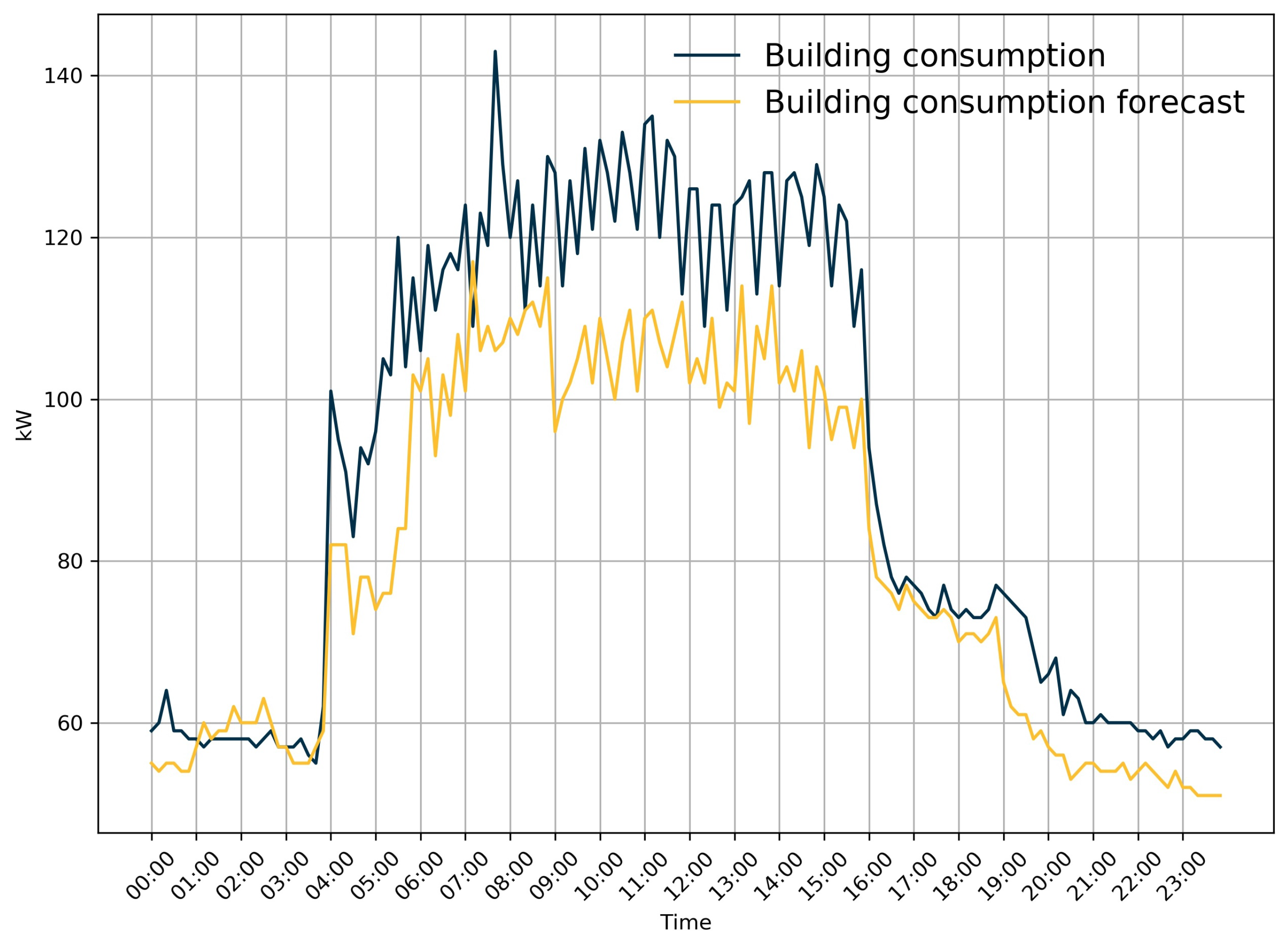
3.1. Optimization of the Forecast for Building Consumption

The pool of V decision variables consists of a subset of historical data ranging from 1 day to 60 days before, while the M objective functions are NRMSDs (see Appendix A), calculated over M different partitions of reference samples. To calculate the NRMSD for a specific individual, we used the Python library sklearn, [33] to generate a model using the individual’s historical data. The model was then evaluated generating multiple forecasts and evaluating them against the M partitions. Results of this process are reported in

Table 1. Six decision variables of the forecast model of building consumption in the optimized case.

	1	2	3	4	5	6
Minutes	0	0	0	0	0	50
Hours	0	0	0	0	0	4
Day	1	7	8	14	15	49

and

Table 2. NRMSD in the 5 different test samples based on the model in Table 1.

1st	$0.048466167003439115$
2nd	$0.049613848265469385$
3rd	$0.04877974896177129$
4th	$0.04987916474341439$
5th	$0.04714514666414881$

. The first lists the six temporal decision variables used to calculate the forecast model, while the second shows the five resulting NRMSDson the various test samples.

$V=6$ and $M=5$ provided the best trade-off between forecast accuracy and computational costs.

Table 3. Decision variables and respective coefficients for the model in Table 1.

Decision Variable	Coefficients	$\mathcal{O}$
1st variable	$0.553957$	${10}^5$
2nd variable	$0.317691$	${10}^4$
3rd variable	$-0.269292$	${10}^4$
4th variable	$0.215163$	${10}^4$
5th variable	$-0.178638$	${10}^4$
6th variable	$-0.023960$	${10}^3$
Temperature	$-1017.701463$	${10}^4$
Wind speed	$-54.743771$	${10}^2$
Humidity	$-246.096902$	${10}^3$
Visibility	$-222.283976$	${10}^3$
Pressure	$-113.217610$	${10}^5$
Cloud cover	$20.999205$	${10}^2$
Dew point	$594.432318$	${10}^4$
UV index	$2089.019033$	${10}^3$

shows all the variables considered in the model described in Table 1 together with the variables indicating weather conditions, and their respective coefficients. To understand which variables are more or less influential for the model, we need to study column $\mathcal{O}$. This column represents the order of magnitude of the decision variable multiplied by its respective coefficient. Holding the convention used in Section 2.3, $\mathcal{O}$ represents the order of magnitude of $b_i{v}_i$$\forall i\in \{0,1,2,\dots ,14\}$. It is worth noting that, due to the random nature of the optimization process, the sixth decision variable refers to the power consumption 49 days, 4 h, and 50 min before our forecast. As one might expect, this variable was the least influential among the decision variables. The table shows how the most influential variables are the power consumption 1 day before the forecast and the air pressure: the first one influences the forecast in a directly proportional manner, the second one in an inversely proportional manner. Finally, cloud cover and wind speed are the least influential in this case.

Figure 8 shows the consumption forecast on date 12 June 2019, calculated applying the model model described in Table 1. In the figure, it is compared with the real consumption of the building on the same day.

3.2. Optimization of the Forecast for PV Production

The same procedure applied in Section 3.1 to predict building consumption has been applied to predict PV production on the same pilot site. The dataset covers the same one-year window with a 10 minutes granularity and was collected using a dedicated smart meter. The optimized model is reported in

Table 4. 6 decision variables of the forecast model of PV production in the optimized case.

	1	2	3	4	5	6
Minutes	0	10	0	0	0	0
Hours	0	0	0	0	0	13
Day	1	1	2	3	5	5

while

Table 5. NRMSD in the 5 different test samples based on the model in Table 4.

1st	$0.06306776095856975$
2nd	$0.0608342720069058$
3rd	$0.06112555224407896$
4th	$0.0609859900027273$
5th	$0.06159178182772625$

reports the related NRMSDs over the five different test partitions. In

Table 6. Decision variables and respective coefficients for the model in Table 4.

Decision Variable	Coefficients	$\mathcal{O}$
1st variable	$0.264537$	${10}^4$
2nd variable	$0.202090$	${10}^4$
3rd variable	$0.143890$	${10}^4$
4th variable	$0.185524$	${10}^4$
5th variable	$0.133130$	${10}^4$
6th variable	$0.001046$	${10}^2$
Temperature	$538.167520$	${10}^4$
Wind speed	$-58.913190$	${10}^2$
Humidity	$46.330959$	${10}^2$
Visibility	$-354.317850$	${10}^3$
Pressure	$3.808337$	${10}^3$
Cloud cover	$-138.965859$	${10}^3$
Dew point	$-848.577608$	${10}^4$
UV index	$550.220030$	${10}^3$

we can see how, in this case, the production can be predicted observing the production of one (exactly one day before and one day and ten minutes before), two, three and five days before, the air temperature, and the dew point. The least influential variables were the production 5 days and 13 hours before, the wind speed, and the humidity. Finally, Figure 9 shows the model in Table 4 applied to forecast the PV production on 12 June 2019.

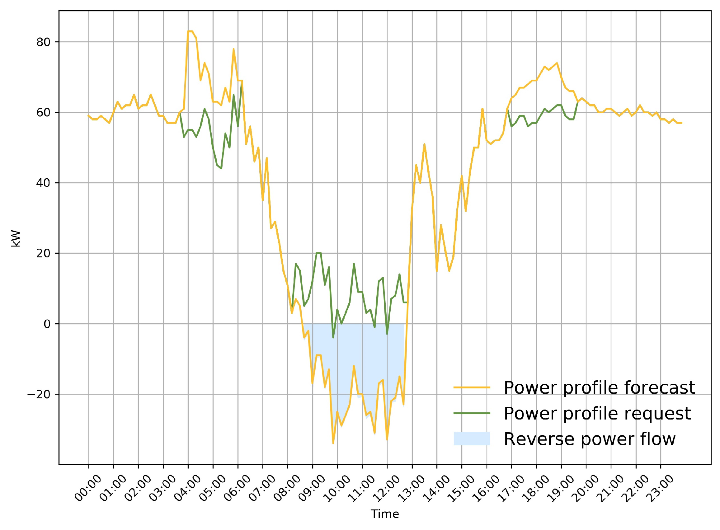
3.3. DSO District Profile Optimization

The two models determined in Section 3.1 and Section 3.2 are combined together to predict the net consumption of the pilot district. The district’s combined power profile can be used then by the DSO to determine its flexibility potential, as is shown in Figure 10 which represents the forecasted power profile on date 12 June 2019 from 00:00 to 23:50.

In the example above, we can see the Reverse Power Flow (RPF) from 08:20 to 12:50 (note the negative consumption) due to an excess of PV production. Moreover, we can see how the peak load is expected from 03:50 to 6:10 and from 17:00 to 19:40. In this scenario, it is reasonable to assume that the DSO in interested in both avoiding the RPF and mitigating the peak loads, together with other considerations related to the overall grid he is managing, so we used this assumption to determine a possible power profile request.

The energy cost was determined by following the commercial offers of retailers currently operating on the market, to obtain a realistic value Figure 11.

A resulting optimized profile is shown in Figure 12. The profile is obtained considering the EV charging schedule in Figure 13 and the power profile to be followed by the battery, with its charging status in Figure 14. As an example, Figure 13 shows that a Renault ZOE, identified here as Car 4, must be recharged from 10:10 to 11:00.

Following the profile in Figure 12, the consumption is reduced by $10.30$ kWh during the peak timeslots (the first one between 3:50 and 6:10 and the second one between 17:00 and 19:40) and the reverse power flow is reduced by $68.64$ kWh, equal to $81.89$% (between 8:20 and 12:50) with a reduction of the peak power of $34.09$ kW (9:50) and significant self-consumption. The DSO considers the mechanism satisfying, the system follows the power profile in most of the cases and the stabilization of the network obtained with the flexibility of the district represents a considerable help reducing the workload of its operations. On the district’s side, the identified profile allowed the 6 EVs to be recharged and awarded the district with $10.00$ incentive tokens, in spite of an additional cost of a mere €$0.88$, proving to be an appealing model.

3.4. Managerial Implications of the Research

The research observed the impact of data-driven optimization of flexibility resources in the context of a distribution network with a high penetration of distributed energy resources. The findings of the research have a number of managerial implications for the actors involved in the scenario. DSO, aggregators, and energy districts should try to increase the use of metering devices capable of integration with data storage and analysis platforms. This will increase the availability of data and thus allow more accurate models to be obtained. Distribution network operators should start to investigate the effects of an increase in the number of electric vehicles circulating and provide for an appropriate incentive plan to involve end-users in flexibility campaigns designed to increase self-consumption and reduce peaks in production from renewable sources and consumption. Companies operating in a district with a high presence of energy from renewable sources could consider encouraging the use of electric vehicles by their employees and act as aggregators by participating in flexibility campaigns.

4. Conclusions

This paper reports on a novel methodology which combines machine learning with multi-objective optimization to find an optimized configuration of different flexibility resources in energy districts with the aim of following a power profile sent by the DSO. The proposed solution is tailored to a real demonstrator located in Terni, Italy, consisting of a district composed of: three passive loads, two RES plants, three EV recharge stations, six electric vehicles and a storage system. Results show that the methodology proposed is satisfactory for both actors in the system: on the DSO side the power profile request is fulfilled with a substantial reduction of reverse power flow, on the district side, the optimized power profile allows to obtain incentives and to reduce operating costs for the fleet of EV. This study has potential limitations, that could be addressed in future research. First, the PV production forecast, based on a single year’s data, does not take into account the degradation rate, which could lead to more accurate long-term forecasts. Second, the power profile optimization could be improved with the integration of social behavior and the integration of the efficiency factor for both the EVs and the storage system.

References

1. Prettico, G.; Flammini, M.G.; Andreadou, N.; Vitiello, S.; Fulli, G.; Masera, M. Distribution System Operators Observatory 2018-Overview of the Electricity Distribution System in Europe; Technical Report EUR 29615EN; Publications Office of the European Union: Luxembourg, 2019. [Google Scholar] [CrossRef]
2. Shoreh, M.H.; Siano, P.; Shafie-khah, M.; Loia, V.; Catalão, J.P. A survey of industrial applications of Demand Response. Electr. Power Syst. Res. 2016, 141, 31–49. [Google Scholar] [CrossRef]
3. Siano, P. Demand response and smart grids—A survey. Renew. Sustain. Energy Rev. 2014, 30, 461–478. [Google Scholar] [CrossRef]
4. Hosseinian Yengejeh, H.; Shahnia, F.; Islam, S. Contributions of single-phase rooftop PVs on short circuits faults in residential feeders. In Proceedings of the 2014 Australasian Universities Power Engineering Conference (AUPEC), Perth, Australia, 28 September–1 October 2014; pp. 1–6. [Google Scholar] [CrossRef] [Green Version]
5. Sarailoo, M.; Akhlaghi, S.; Rezaeiahari, M.; Sangrody, H. Residential solar panel performance improvement based on optimal intervals and optimal tilt angle. In Proceedings of the 2017 IEEE Power Energy Society General Meeting, Chicago, IL, USA, 16–20 July 2017; pp. 1–5. [Google Scholar]
6. Li, Y.; Wang, C.; Li, G.; Wang, J.; Zhao, D.; Chen, C. Improving operational flexibility of integrated energy system with uncertain renewable generations considering thermal inertia of buildings. Energy Convers. Manag. 2020, 207, 112526. [Google Scholar] [CrossRef] [Green Version]
7. Ghasemi, A.; Enayatzare, M. Optimal energy management of a renewable-based isolated microgrid with pumped-storage unit and demand response. Renew. Energy 2018, 123, 460–474. [Google Scholar] [CrossRef]
8. Gils, H. Balancing of Intermittent Renewable Power Generation by Demand Response and Thermal Energy Storage. Ph.D. Thesis, University of Stuttgart, Stuttgart, Germany, 2015. [Google Scholar]
9. Lorenzi, G.; Silva, C.A.S. Comparing demand response and battery storage to optimize self-consumption in PV systems. Appl. Energy 2016, 180, 524–535. [Google Scholar] [CrossRef]
10. Knezovic, K.; Marinelli, M.; Perez, y.; Codani, P. Distribution Grid Services and Flexibility Provision by Electric Vehicles: a Review of Options. In Proceedings of the 2015 50th International Universities Power Engineering Conference (UPEC), Stoke on Trent, UK, 1–4 September 2015; pp. 1–6. [Google Scholar] [CrossRef] [Green Version]
11. Bragatto, T.; Cresta, M.; Croce, V.; Paulucci, M.; Santori, F.; Ziu, D. A real-life experience on 2nd life batteries services for Distribution System Operator. In Proceedings of the 2019 IEEE International Conference on Environment and Electrical Engineering and 2019 IEEE Industrial and Commercial Power Systems Europe (EEEIC / I CPS Europe), Genova, Italy, 11–14 June 2019; pp. 1–6. [Google Scholar]
12. Luca de Tena, D. Large Scale Renewable Power Integration with Electric Vehicles: Long Term Analysis for Germany with a Renewable Based Power Supply. Ph.D. Thesis, Universität Stuttgart, Stuttgart, Germany, 2014. [Google Scholar]
13. Cheng, C.; Pourhejazy, P.; Ying, K.; Li, S.; Chang, C. Learning-Based Metaheuristic for Scheduling Unrelated Parallel Machines With Uncertain Setup Times. IEEE Access 2020, 8, 74065–74082. [Google Scholar] [CrossRef]
14. Sofia, A.; GaneshKumar, P. Multi-objective Task Scheduling to Minimize Energy Consumption and Makespan of Cloud Computing Using NSGA-II. J. Netw. Syst. Manag. 2017, 26, 1–23. [Google Scholar] [CrossRef]
15. Nascimento, Z.; Sadok, D.; Fernandes, S.; Kelner, J. Multi-objective optimization of a hybrid model for network traffic classification by combining machine learning techniques. In Proceedings of the 2014 International Joint Conference on Neural Networks (IJCNN), Beijing, China, 6–11 July 2014; pp. 2116–2122. [Google Scholar]
16. Mellit, A.; Kalogirou, S.A. Artificial intelligence techniques for photovoltaic applications: A review. Prog. Energy Combust. Sci. 2008, 34, 574–632. [Google Scholar] [CrossRef]
17. Seyedzadeh, S.; Pour Rahimian, F.; Glesk, I.; Roper, M. Machine learning for estimation of building energy consumption and performance: A review. Vis. Eng. 2018, 6. [Google Scholar] [CrossRef]
18. Bogner, K.; Pappenberger, F.; Zappa, M. Machine Learning Techniques for Predicting the Energy Consumption/Production and Its Uncertainties Driven by Meteorological Observations and Forecasts. Sustainability 2019, 11, 3328. [Google Scholar] [CrossRef] [Green Version]
19. Voyant, C.; Notton, G.; Kalogirou, S.; Nivet, M.L.; Paoli, C.; Motte, F.; Fouilloy, A. Machine learning methods for solar radiation forecasting: A review. Renew. Energy 2017, 105, 569–582. [Google Scholar] [CrossRef]
20. Deb, K.; Pratap, A.; Agarwal, S.; Meyarivan, T. A fast and elitist multiobjective genetic algorithm: NSGA-II. Mathematics 2002, 6, 182–197. [Google Scholar] [CrossRef] [Green Version]
21. Junior, B.; Cossi, A.; Mantovani, J. Multiobjective Short-Term Planning of Electric Power Distribution Systems Using NSGA-II. J. Control. Autom. Electr. Syst. 2013, 24. [Google Scholar] [CrossRef]
22. Attari, S.; Shakarami, M.; Pour, E. Pareto optimal reconfiguration of power distribution systems with load uncertainty and recloser placement simultaneously using a genetic algorithm based on NSGA-II. In Proceedings of the 2016 21st Conference on Electrical Power Distribution Networks Conference (EPDC), Karaj, Iran, 26–27 April 2016; pp. 46–53. [Google Scholar] [CrossRef]
23. Buoro, D.; Casisi, M.; Nardi, A.D.; Pinamonti, P.; Reini, M. Multicriteria optimization of a distributed energy supply system for an industrial area. Energy 2013, 58, 128–137. [Google Scholar] [CrossRef]
24. Ippolito, M.; Silvestre, M.D.; Sanseverino, E.R.; Zizzo, G.; Graditi, G. Multi-objective optimized management of electrical energy storage systems in an islanded network with renewable energy sources under different design scenarios. Energy 2014, 64, 648–662. [Google Scholar] [CrossRef]
25. FIWARE. Available online: https://www.fiware.org (accessed on 20 April 2020).
26. Amber, K.; Aslam, M.; Hussain, S. Electricity consumption forecasting models for administration buildings of the UK higher education sector. Energy Build. 2015, 90, 127–136. [Google Scholar] [CrossRef]
27. Braun, M.; Altan, H.; Beck, S. Using regression analysis to predict the future energy consumption of a supermarket in the UK. Appl. Energy 2014, 130, 305–313. [Google Scholar] [CrossRef] [Green Version]
28. Al-Garni, A.Z.; Zubair, S.M.; Nizami, J.S. A regression model for electric-energy-consumption forecasting in Eastern Saudi Arabia. Energy 1994, 19, 1043–1049. [Google Scholar] [CrossRef]
29. Chen, C.; Duan, S.; Cai, T.; Liu, B. Online 24-h solar power forecasting based on weather type classification using artificial neural network. Solar Energy 2011, 85, 2856–2870. [Google Scholar] [CrossRef]
30. Nguyen, D.; Lehman, B.; Kamarthi, S. Performance evaluation of solar photovoltaic arrays including shadow effects using neural network. In Proceedings of the 2009 IEEE Energy Conversion Congress and Exposition, San Jose, CA, USA, 20–24 September 2009; pp. 3357–3362. [Google Scholar] [CrossRef]
31. Hiyama, T.; Kitabayashi, K. Neural network based estimation of maximum power generation from PV module using environmental information. IEEE Trans. Energy Convers. 1997, 12, 241–247. [Google Scholar] [CrossRef]
32. World Weather Online. Available online: https://www.worldweatheronline.com (accessed on 16 April 2020).
33. Pedregosa, F.; Varoquaux, G.; Gramfort, A.; Michel, V.; Thirion, B.; Grisel, O.; Blondel, M.; Prettenhofer, P.; Weiss, R.; Dubourg, V.; et al. Scikit-learn: Machine Learning in Python. J. Mach. Learn. Res. 2012, 12, 2825–2830. [Google Scholar]
34. Deb, K.; Jain, H. An Evolutionary Many-Objective Optimization Algorithm Using Reference-Point-Based Nondominated Sorting Approach, Part I: Solving Problems With Box Constraints. IEEE Trans. Evol. Comput. 2014, 18, 577–601. [Google Scholar] [CrossRef]
35. Ishibuchi, H.; Imada, R.; Setoguchi, Y.; Nojima, Y. Performance comparison of NSGA-II and NSGA-III on various many-objective test problems. In Proceedings of the 2016 IEEE Congress on Evolutionary Computation (CEC), Vancouver, BC, Canada, 24–29 July 2016; pp. 3045–3052. [Google Scholar]
36. Farmani, R.; Savic, D.; Walters, G. Multi-objective optimization of water system: a comparative study. Pumps Electromech. Devices Syst. Appl. Urban Water Manag. 2003, 1, 247–256. [Google Scholar]
37. D’Oriano, L.; Mastandrea, G.; Rana, G.; Raveduto, G.; Croce, V.; Verber, M.; Bertoncini, M. Decentralized blockchain flexibility system for Smart Grids: Requirements engineering and use cases. In Proceedings of the 2018 International IEEE Conference and Workshop in Óbuda on Electrical and Power Engineering (CANDO-EPE), Budapest, Hungary, 20–21 November 2018; pp. 39–44. [Google Scholar]
Figure 1. This figure shows the graphic representation of the pilot district.
Electronics 09 00945 g001
Figure 2. This figure describes the software architecture and the services used in our prototype implementation.
Electronics 09 00945 g002
Figure 3. This figure shows the process to generate forecasts from raw historical data.
Electronics 09 00945 g003
Figure 4. Normalized Root Mean Squared Deviation (NRMSD) % evolution according to population size, crossover and mutation rates.
Electronics 09 00945 g004
Figure 5. NRMSD % evolution according to the number of generations.
Electronics 09 00945 g005
Figure 6. Reverse Power Flow (RPF) % evolution according to population size, crossover and mutation rates.
Electronics 09 00945 g006
Figure 7. RPF % evolution according to the number of generations.
Electronics 09 00945 g007
Figure 8. This figure shows the building consumption on 12 June 2019. The forecast shown is based on the model in Table 1.
Electronics 09 00945 g008
Figure 9. This figure shows the photovoltaics (PV) production on 12 June 2019. The forecast shown is based on the model in Table 4.
Electronics 09 00945 g009
Figure 10. This figure shows a possible scenario for flexibility provisioning.
Electronics 09 00945 g010
Figure 11. This figure shows how the price of energy varies over the course of a day.
Electronics 09 00945 g011
Figure 12. This figure shows a possible optimized profile given the request shown in Figure 10.
Electronics 09 00945 g012
Figure 13. Vehicle recharging schedule for the profile in Figure 12.
Electronics 09 00945 g013
Figure 14. Energy storage system power profile for the profile in Figure 12.
Electronics 09 00945 g014